Proportional-Type Performance Recovery DC-Link Voltage Tracking Algorithm for Permanent Magnet Synchronous Generators

Abstract

This study proposes a disturbance observer-based proportional-type DC-link voltage tracking algorithm for permanent magnet synchronous generators (PMSGs). The proposed technique feedbacks the only proportional term of the tracking errors, and it contains the nominal static and dynamic feed-forward compensators coming from the first-order disturbance observers. It is rigorously proved that the proposed method ensures the performance recovery and offset-free properties without the use of the integrators of the tracking errors. A wind power generation system has been simulated to verify the efficacy of the proposed method using the PSIM (PowerSIM) software with the DLL (Dynamic Link Library) block.

1. Introduction

Because of the high efficiency, high power, and simple structures, the use of permanent magnet synchronous machines (PMSMs) for various motoring and generating applications has been preferred. Eliminating the external rotor excitation removes the rotor losses, which improves the PMSM efficiency dramatically. Moreover, the absence of rotor winding eliminates not only the slip rings but also the brushes, which leads to a considerable reduction of the maintenance costs [1,2,3,4,5,6].

In power generating applications, the PMSM plays the role of a balanced three-phase AC power supply depending on the input mechanical power source, such as wind power, thermoelectric power, nuclear power, and so on. The DC-link voltage across the output capacitor should be controlled by the three-phase inverter with properly designed control algorithms. Because the corresponding DC-link voltage control problem of the PMSM-based power system is equivalent to the case of the AC/DC converter with a variable AC power source, the extant solutions for the AC/DC converter output voltage control problems can be applied. The cascade control strategy has mainly been adopted for controlling the output voltage of AC/DC converters, where the outer-loop controller produces a desired d-axis current reference for the inner-loop current controller so as to regulate the output voltage. Because of the simple structure, the proportional-integral (PI) controller has commonly been used for the both inner and outer loops [7]. In the AC/DC converter model, there exist inherent nonlinearities and disturbance terms in the output voltage and current dynamics, which could cause a severe closed-loop degradation or instability. Several novel control techniques have been applied for developing the inner-loop current controller to improve the output voltage tracking performance by dealing with the nonlinearities and disturbance terms accordingly. For instance, feedback-linearizing [8,9], passivity-based [10], and predictive [11] schemes remarkably enhanced the closed-loop performance by canceling the nonlinearity and disturbances using the true parameters of the AC/DC converter. The model predictive controllers (MPCs) in [12] were designed to try to enhance the transient performance through minimizing the cost function tracking errors, by using an exhaustive search method for each sampling time. These advanced methods, however, require the use of the true parameters of the converter, such as the resistance, inductance, and capacitance, to ensure closed-loop stability with the desired closed-loop performance. Thus, it is questionable that these advanced schemes can still provide the desired closed-loop performance with the stability guarantee, as the converter parameters and the load current can be dramatically changed in accordance with the operating conditions. An adaptive current controller in [13] has been devised in order to deal with the parameter uncertainties, but it is ambiguous whether the current convergence property is still valid without an offset error in the real implementation due to the absence of the integrators in the tracking errors. The recent sliding mode controller in [14] was developed in order to enhance the output voltage tracking performance in the transient periods by suppressing the disturbance terms caused by a plant-model mismatch. In the case of the proportional type output voltage controller in [15], there were no stability analysis and steady-state analysis with respect to the offset errors. Disturbance observer (DOB)-based output voltage controllers are used in [16,17] that include the integrators of the tracking errors, which may require the use of anti-windup algorithms.

There have been many multi-variable approaches in [18,19,20,21] to solve the output voltage tracking problem of the AC/DC converter. These methods have been made through two steps; first, a positive definite function with respect to the tracking errors was defined, and second, a control action was derived to make the positive definite function monotonically decreasing for all time. However, knowledge of the true parameters is required to ensure the closed-loop performances.

This paper offers a DOB-based proportional-type DC-link voltage tracking algorithm, considering the nonlinearity in the DC-link voltage and PMSM dynamics with the model-plant mismatches. The proposed method is derived through a multi-variable approach, which combines the simple proportional-type feedback linearizing (FL) controller with the first-order DOBs. The contribution of this article is summarized as follows. First, it incorporates the first-order DOBs in the proportional-type FL DC-link voltage control algorithm so as to stabilize the tracking errors. Second, it is rigorously proved that the closed-loop system ensures the performance recovery property as well as the offset-free property without the use of the integrators of the tracking errors. The realistic simulation results confirm the efficacy of the proposed method, in which the wind power system with the output capacitor has been emulated by PSIM (PowerSIM) software.

2. Permanent Magnet Synchronous Generator Model in Rotational d-q Axis

In the rotational d-q axis, the electrical and mechanical dynamics of the permanent magnet synchronous generator (PMSG) are given by [22]:

$$\begin{array}{c}\hfill L_d\frac{d{i}_d\left(t\right)}{dt}=-R_s{i}_d\left(t\right)+L_q{\omega }_r\left(t\right)i_q\left(t\right)+u_d\left(t\right)\end{array}$$

(1)

$$\begin{array}{c}\hfill L_q\frac{d{i}_q\left(t\right)}{dt}=-R_s{i}_q\left(t\right)-L_d{\omega }_r\left(t\right)i_d\left(t\right)-{\lambda }_{PM}{\omega }_r\left(t\right)+u_q\left(t\right)\end{array}$$

(2)

$$\begin{array}{ccc}J\frac{d\omega \left(t\right)}{dt}\hfill & =\hfill & -B\omega \left(t\right)+T_m\left(t\right)-T_e(i_d\left(t\right),i_q\left(t\right)),\hfill \end{array}$$

(3)

$\forall t\ge 0$, where $i_d\left(t\right)$, $i_q\left(t\right)$, and ${\omega }_r\left(t\right):=P\omega \left(t\right)$ denote the d-q axis’ current and electrical speed, respectively, and $\omega \left(t\right)$ and P represent the mechanical speed and the number of pole pairs, respectively. The PMSG parameters $R_s$, $L_d$, $L_q$, ${\lambda }_{PM}$, B, and J represent the stator resistance, d-q inductances, magnet flux, viscous friction, and rotor moment of inertia, respectively, and $T_m\left(t\right)$ is the input mechanical torque. The input voltages $u_d\left(t\right)$ and $u_q\left(t\right)$ are treated as the control input, and the electrical torque $T_e(i_d\left(t\right),i_q\left(t\right))$ is given by

$$T_e(i_d\left(t\right),i_q\left(t\right)):=\frac{3}{2}P\left(\Delta L_{dq}{i}_d\left(t\right)i_q\left(t\right)+{\lambda }_{PM}{i}_q\left(t\right)\right),\forall t\ge 0$$

(4)

where $\Delta L_{dq}:=L_d-L_q$.

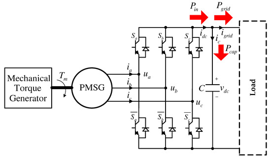
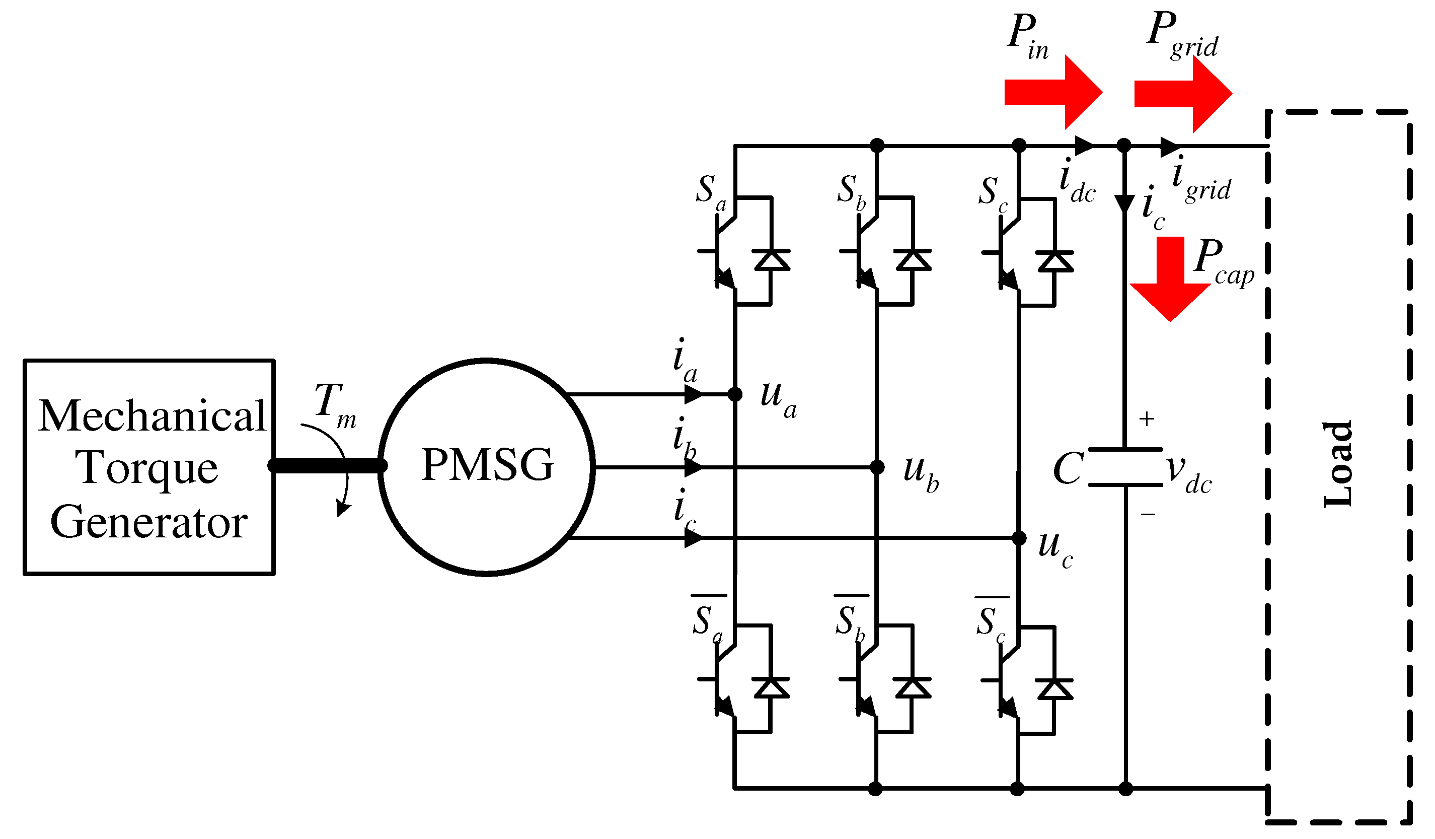
Letting $P_{cap}\left(t\right)$, $P_{in}\left(t\right)$, and $P_{grid}\left(t\right)$ be the capacitor power, input power, and grid power, respectively, as shown in Figure 1, it holds that

$$\begin{array}{c}\hfill P_{cap}\left(t\right)=C{v}_{dc}\left(t\right)\frac{d{v}_{dc}\left(t\right)}{dt}=P_{in}\left(t\right)-P_{grid}\left(t\right),\forall t\ge 0\end{array}$$

(5)

and, because the input power of $P_{in}\left(t\right)$ can be decomposed as $P_{in}\left(t\right)=P_G\left(t\right)+P_{loss,inv}\left(t\right)$, $\forall t\ge 0$, where $P_G\left(t\right)$ and $P_{loss,inv}\left(t\right)$ are the generator output power and the inverter power loss, respectively, it follows from Equation (5) that

$$\begin{array}{c}\hfill C\frac{d{v}_{dc}\left(t\right)}{dt}=\frac{\omega \left(t\right)}{v_{dc}\left(t\right)}{T}_e\left(t\right)+\frac{P_{loss,inv}\left(t\right)}{v_{dc}\left(t\right)}-I_{grid}\left(t\right),\forall t\ge 0\end{array}$$

(6)

where $I_{grid}\left(t\right)$ denotes the load current to the grid.

Figure 1. The permanent magnet synchronous generator (PMSG) power system topology.

It should be noted that it is difficult to consistently identify the true values of the PMSG parameters, with the exception of the number of pole pairs P as well as the output capacitance value, because the parameters can dramatically vary with the operating conditions, such as the phase current, DC-link voltage, and PMSG temperature. Thus, it is reasonable for the dynamical Equations (1), (2), and (6) to be rewritten as

$$\begin{array}{ccc}\hfill L_{d,0}\frac{d{i}_d\left(t\right)}{dt}& =& -R_{s,0}{i}_d\left(t\right)+L_{q,0}{\omega }_r\left(t\right)i_q\left(t\right)\hfill \\ & & +u_d\left(t\right)+d_{d,o}\left(t\right)\hfill \end{array}$$

(7)

$$\begin{array}{ccc}\hfill L_{q,0}\frac{d{i}_q\left(t\right)}{dt}& =& -R_{s,0}{i}_q\left(t\right)-L_{d,0}{\omega }_r\left(t\right)i_d\left(t\right)-{\lambda }_{PM,0}{\omega }_r\left(t\right)\hfill \\ & & +u_q\left(t\right)+d_{q,o}\left(t\right)\hfill \end{array}$$

(8)

$$\begin{array}{ccc}\hfill C_0\frac{d{v}_{dc}\left(t\right)}{dt}& =& \frac{\omega \left(t\right)}{v_{dc}\left(t\right)}{T}_{e,0}\left(t\right)+d_{v,o}\left(t\right),\forall t\ge 0\hfill \end{array}$$

(9)

with the nominal parameters of $R_{s,0}$, $L_{d,0}$, $L_{q,0}$, ${\lambda }_{PM,0}$, and $C_0$, where the nominal torque $T_{e,0}\left(t\right)$ is defined as

$$T_{e,0}\left(t\right):=T_e\left(t\right){|}_{L_d=L_{d,0},L_q=L_{q,0},{\lambda }_{PM}={\lambda }_{PM,0}},\forall t\ge 0$$

and $d_{d,o}\left(t\right)$, $d_{q,o}\left(t\right)$, and $d_{v,o}\left(t\right)$ denote the unknown disturbances caused from the parameter mismatch, unmodeled dynamics, and load uncertainties.

The next section develops a DC-link voltage tracking algorithm based on the perturbed PMSG current dynamics of Equations (7) and (8) with the DC-link voltage dynamics of Equation (9). To this end, the following assumptions are made:

• The disturbances $d_{d,o}\left(t\right)$, $d_{q,o}\left(t\right)$, and $d_{v,o}\left(t\right)$ are unknown, but their time-derivatives are bounded for all time.
• The stationary a-b-c phase current and the PMSG speed $\omega \left(t\right)$ are measurable so that the rotational d-q axis currents are available for feedback.

3. DC-Link Voltage Tracking Algorithm Design

The DC-link voltage control objective is to force the closed-loop system to behave according to the transfer function given by

$$\begin{array}{c}\hfill \frac{V_{dc}^{*}\left(s\right)}{V_{dc,ref}\left(s\right)}=\frac{{\omega }_{vc}}{s+{\omega }_{vc}},\forall s\in \mathbb{C}\end{array}$$

(10)

where ${\omega }_{vc}$ is the desired cut-off frequency as a design parameter, and $V_{dc}^{*}\left(s\right)$ and $V_{dc,ref}\left(s\right)$ denote the Laplace transforms of the DC-link voltage $v_{dc}^{*}\left(t\right)$ and its reference $v_{dc,ref}\left(t\right)$, respectively.

The time domain expression of the target dynamics of Equation (10) can be written as

$$\begin{array}{c}\hfill {\dot{v}}_{dc}^{*}\left(t\right)={\omega }_{vc}\left(v_{dc,ref}\left(t\right)-v_{dc}^{*}\left(t\right)\right),\forall t\ge 0\end{array}$$

(11)

and, then, with the target dynamics of Equation (11), defining the error as

$${\tilde{v}}_{dc}^{*}\left(t\right):=v_{dc}^{*}\left(t\right)-v_{dc}\left(t\right),\forall t\ge 0$$

the DC-link voltage tracking error dynamics can be obtained as

$$\begin{array}{ccc}\hfill C_0{\dot{\tilde{v}}}_{dc}^{*}\left(t\right)& =& C_0{\dot{v}}_{dc}^{*}\left(t\right)-C_0{\dot{v}}_{dc}\left(t\right)\hfill \\ & =& -\frac{\omega \left(t\right)}{v_{dc}\left(t\right)}b{i}_q\left(t\right)-\frac{\omega \left(t\right)}{v_{dc}\left(t\right)}\frac{3}{2}P\Delta L_{dq,0}{i}_d\left(t\right)i_q\left(t\right)+d_v\left(t\right)\hfill \\ & =& -\frac{\omega \left(t\right)}{v_{dc}\left(t\right)}b{i}_{q,ref}\left(t\right)+\frac{\omega \left(t\right)}{v_{dc}\left(t\right)}b{\tilde{i}}_q\left(t\right)\hfill \\ & & -\frac{\omega \left(t\right)}{v_{dc}\left(t\right)}\frac{3}{2}P\Delta L_{dq,0}{i}_d\left(t\right)i_q\left(t\right)+d_v\left(t\right),\forall t\ge 0\hfill \end{array}$$

(12)

where $b:=\frac{3}{2}P{\lambda }_{PM,0}$, $i_{q,ref}\left(t\right)$ denotes the q-axis current reference, the q-axis current tracking error ${\tilde{i}}_q\left(t\right)$ is defined as ${\tilde{i}}_q\left(t\right):=i_{q,ref}\left(t\right)-i_q\left(t\right)$, $\forall t\ge 0$, $L_{dq,0}:=L_{dq}{|}_{L_d,L_q=L_{d,0},L_{q,0}}$, and $d_v\left(t\right):=C_0{\dot{v}}_{dc}^{*}\left(t\right)-d_{v,o}\left(t\right)$, $\forall t\ge 0$.

The stabilization of the tracking error dynamics of Equation (12) can be established by the proposed q-axis current reference:

$$\begin{array}{c}\hfill i_{q,ref}\left(t\right):=\frac{v_{dc}\left(t\right)}{b\omega \left(t\right)}\left(C_0{\lambda }_{vc}{\tilde{v}}_{dc}^{*}\left(t\right)-\frac{\omega \left(t\right)}{v_{dc}\left(t\right)}\frac{3}{2}P\Delta L_{dq,0}{i}_d\left(t\right)i_q\left(t\right)+{\widehat{d}}_v\left(t\right)\right),\forall t\ge 0\end{array}$$

(13)

where ${\lambda }_{vc}>0$ refers to the design parameter for adjusting the decay ratio of the DC-link voltage tracking error of ${\tilde{v}}_{dc}^{*}\left(t\right)$, and ${\widehat{d}}_v\left(t\right)$ represents the estimated disturbance defined as

$$\begin{array}{c}\hfill {\widehat{d}}_v\left(t\right):={\zeta }_v\left(t\right)+l_v{C}_0{\tilde{v}}_{dc}^{*}\left(t\right),\forall t\ge 0\end{array}$$

(14)

The state ${\zeta }_v\left(t\right)$ satisfies the nonlinear observer dynamics:

$$\begin{array}{c}\hfill {\dot{\zeta }}_v\left(t\right)=-l_v{\zeta }_v\left(t\right)-l_v^2{C}_0{\tilde{v}}_{dc}^{*}\left(t\right)+l_v\frac{\omega \left(t\right)}{v_{dc}\left(t\right)}\left(b{i}_q\left(t\right)+\frac{3}{2}P\Delta L_{dq,0}{i}_d\left(t\right)i_q\left(t\right)\right),\forall t\ge 0\end{array}$$

(15)

where $l_v>0$ is the observer gain as a design parameter. For the rest of this article, the nonlinear observer of Equation (15) with the output of Equation (14) is called the DC-link voltage DOB.

Substitution of the proposed q-axis current reference of Equation (13) to the DC-link voltage error dynamics of Equation (12) yields that

$$\begin{array}{c}\hfill {\dot{\tilde{v}}}_{dc}^{*}\left(t\right)=-{\lambda }_{vc}{\tilde{v}}_{dc}^{*}\left(t\right)+\frac{\omega \left(t\right)}{C_0{v}_{dc}\left(t\right)}b{\tilde{i}}_q\left(t\right)+\frac{1}{C_0}{\tilde{d}}_v\left(t\right),\forall t\ge 0\end{array}$$

(16)

where ${\tilde{d}}_v\left(t\right):=d_v\left(t\right)-{\widehat{d}}_v\left(t\right)$, $\forall t\ge 0$. Lemma 1 presents the stability property of the closed-loop error dynamics of Equation (16), which helps the whole closed-loop stability analysis to be performed considerably easily.

Lemma 1.

For any specified designed parameters ${\lambda }_{vc}>0$ and $l_v>0$, the proposed q-axis current reference of Equation (13) forces the DC-link voltage error dynamics of Equation (16) to be strictly passive with respect to the input–output mapping given by

$$\begin{array}{c}\hfill \left[\begin{array}{c}\frac{\omega \left(t\right)}{C_0{v}_{dc}\left(t\right)}b{\tilde{i}}_q\left(t\right)\\ {\gamma }_v{\dot{d}}_v\left(t\right)\end{array}\right]\mapsto \left[\begin{array}{c}{\tilde{v}}_{dc}^{*}\left(t\right)\\ {\tilde{d}}_v\left(t\right)\end{array}\right]\end{array}$$

(17)

for some positive constant ${\gamma }_v$.

The result of Lemma 1 implies that the DC-link voltage of $v_{dc}\left(t\right)$ exponentially converges to the target trajectory of $v_{dc}^{*}\left(t\right)$ if the two signals of ${\tilde{i}}_q\left(t\right)$ and ${\dot{d}}_v\left(t\right)$ exponentially vanish. The Appendix A proves Lemma 1 by showing the positive definite function, defined as

$$\begin{array}{c}\hfill V_{v_{dc}}\left(t\right):=\frac{1}{2}{\left({\tilde{v}}_{dc}^{*}\left(t\right)\right)}^2+\frac{{\gamma }_v}{2}{\tilde{d}}_v^2\left(t\right),\forall t\ge 0\end{array}$$

(18)

to be

$$\begin{array}{c}\hfill {\dot{V}}_{v_{dc}}\left(t\right)\le -{\alpha }_{v_{dc}}{V}_{v_{dc}}\left(t\right)+{\tilde{v}}_{dc}^{*}\left(t\right)\frac{\omega \left(t\right)}{C_0{v}_{dc}\left(t\right)}b{\tilde{i}}_q\left(t\right)+{\gamma }_v{\tilde{d}}_v\left(t\right){\dot{d}}_v\left(t\right),\forall t\ge 0\end{array}$$

(19)

for some constants ${\alpha }_{v_c}>0$ and ${\gamma }_v>0$. For details, see the Appendix A.

The next step is to derive the d-q axis current error dynamics, which can be obtained as

$$\begin{array}{ccc}\hfill L_{d,0}{\dot{\tilde{i}}}_d\left(t\right)& =& L_{d,0}{\dot{i}}_{d,ref}\left(t\right)-L_{d,0}{\dot{i}}_d\left(t\right)\hfill \\ & =& R_{s,0}{i}_d\left(t\right)-L_{q,0}{\omega }_r\left(t\right)i_q\left(t\right)-u_d\left(t\right)+d_d\left(t\right)\hfill \end{array}$$

(20)

$$\begin{array}{ccc}\hfill L_{q,0}{\dot{\tilde{i}}}_q\left(t\right)& =& L_{q,0}{\dot{i}}_{q,ref}\left(t\right)-L_{q,0}{\dot{i}}_q\left(t\right)\hfill \\ & =& R_{s,0}{i}_q\left(t\right)+L_{d,0}{\omega }_r\left(t\right)i_d\left(t\right)+{\lambda }_{PM,0}{\omega }_r\left(t\right)\hfill \\ & & -u_q\left(t\right)+d_q\left(t\right)\hfill \end{array}$$

(21)

where

$$\begin{array}{ccc}\hfill d_d\left(t\right)& :=& L_{d,0}{\dot{i}}_{d,ref}\left(t\right)-d_{d,o}\left(t\right)\hfill \\ \hfill d_q\left(t\right)& :=& L_{q,0}{\dot{i}}_{q,ref}\left(t\right)-d_{q,o}\left(t\right),\forall t\ge 0\hfill \end{array}$$

For stabilizing the error dynamics of Equations (16), (20) and (21), the control law is proposed as

$$\begin{array}{ccc}\hfill u_d\left(t\right)& =& R_{s,0}{i}_d\left(t\right)-L_{q,0}{\omega }_r\left(t\right)i_q\left(t\right)+L_{d,0}{\lambda }_{cc}{\tilde{i}}_d\left(t\right)+{\widehat{d}}_d\left(t\right)\hfill \end{array}$$

(22)

$$\begin{array}{ccc}\hfill u_q\left(t\right)& =& R_{s,0}{i}_q\left(t\right)+L_{d,0}{\omega }_r\left(t\right)i_d\left(t\right)+{\lambda }_{PM,0}{\omega }_r\left(t\right)+\frac{L_{q,0}\omega \left(t\right)}{C_0{v}_{dc}\left(t\right)}b{\tilde{v}}_{dc}^{*}\hfill \\ & & +L_{q,0}{\lambda }_{cc}{\tilde{i}}_q\left(t\right)+{\widehat{d}}_q\left(t\right),\forall t\ge 0\hfill \end{array}$$

(23)

where the design parameter ${\lambda }_{cc}>0$ is introduced to tune the decay ratio of the current tracking errors ${\tilde{i}}_x\left(t\right)$, $x=d,q$; the estimated disturbances, ${\widehat{d}}_x\left(t\right)$, $x=d,q$, are defined as

$$\begin{array}{c}\hfill {\widehat{d}}_x\left(t\right):={\zeta }_x\left(t\right)+l_x{L}_{x,0}{\tilde{i}}_x\left(t\right),x=d,q,\forall t\ge 0\end{array}$$

(24)

and ${\zeta }_x\left(t\right)$, $x=d,q$ denote the states of the nonlinear observers:

$$\begin{array}{ccc}\hfill {\dot{\zeta }}_d\left(t\right)& =& -l_d{\zeta }_d\left(t\right)-l_d^2{L}_{d,0}{\tilde{i}}_d\left(t\right)\hfill \\ & & +l_d\left(-R_{s,0}{i}_d\left(t\right)+L_{q,0}{\omega }_r\left(t\right)i_q\left(t\right)+u_d\left(t\right)\right)\hfill \end{array}$$

(25)

$$\begin{array}{ccc}\hfill {\dot{\zeta }}_q\left(t\right)& =& -l_q{\zeta }_q\left(t\right)-l_q^2{L}_{q,0}{\tilde{i}}_q\left(t\right)\hfill \\ & & +l_q\left(-R_{s,0}{i}_q\left(t\right)-L_{d,0}{\omega }_r\left(t\right)i_d\left(t\right)-{\lambda }_{PM,0}{\omega }_r\left(t\right)+u_q\left(t\right)\right),\forall t\ge 0\hfill \end{array}$$

(26)

where $l_x>0$, $x=d,q$ are the observer gains as design parameters. For the rest of this article, the nonlinear observers of Equations (25) and (26) with the outputs of Equation (24) are called the current DOBs.

Substituting the control laws of Equations (22) and (23) to the d-q current error dynamics of Equations (20) and (21), it is easy to see that

$$\begin{array}{ccc}\hfill {\dot{\tilde{i}}}_d\left(t\right)& =& -{\lambda }_{cc}{\tilde{i}}_d\left(t\right)+\frac{1}{L_{d,0}}{\tilde{d}}_d\left(t\right)\hfill \end{array}$$

(27)

$$\begin{array}{ccc}\hfill {\dot{\tilde{i}}}_q\left(t\right)& =& -{\lambda }_{cc}{\tilde{i}}_q\left(t\right)-\frac{\omega \left(t\right)}{C_0{v}_{dc}\left(t\right)}b{\tilde{v}}_{dc}^{*}\left(t\right)+\frac{1}{L_{q,0}}{\tilde{d}}_q\left(t\right),\forall t\ge 0\hfill \end{array}$$

(28)

where ${\tilde{d}}_x\left(t\right):=d_x\left(t\right)-{\widehat{d}}_x\left(t\right)$ and $x=d,q$, $\forall t\ge 0$. Lemma 2 presents the stability property of the closed-loop error dynamics of Equations (27) and (28), which helps the whole closed-loop stability analysis to be performed considerably easily.

Lemma 2.

For any specified designed parameters ${\lambda }_{cc}>0$, $l_x>0$ and $x=d,q$, the proposed control law of Equations (22) and (23) forces the d-q axis error dynamics of Equations (27) and (28) to be strictly passive with respect to the input–output mapping given by

$$\begin{array}{c}\hfill \left[\begin{array}{c}0\\ -\frac{\omega \left(t\right)}{C_0{v}_{dc}\left(t\right)}b{\tilde{v}}_{dc}^{*}\left(t\right)\\ {\gamma }_d{\dot{d}}_d\left(t\right)\\ {\gamma }_q{\dot{d}}_q\left(t\right)\end{array}\right]\mapsto \left[\begin{array}{c}{\tilde{i}}_d\left(t\right)\\ {\tilde{i}}_q\left(t\right)\\ {\tilde{d}}_d\left(t\right)\\ {\tilde{d}}_q\left(t\right)\end{array}\right]\end{array}$$

(29)

for some positive constants ${\gamma }_x$, $x=d,q$.

The result of Lemma 2 implies that the d-q axis current tracking errors exponentially vanish if the signals of ${\tilde{v}}_{dc}^{*}\left(t\right)$ and ${\dot{d}}_x\left(t\right)$, $x=d,q$ also vanish. The Appendix A proves Lemma 2 by showing the positive definite function defined as

$$\begin{array}{c}\hfill V_{dq}\left(t\right):=\sum _{x=d,q}\frac{1}{2}{\tilde{i}}_x^2\left(t\right)+\sum _{x=d,q}\frac{{\gamma }_x}{2}{\tilde{d}}_x^2\left(t\right),\forall t\ge 0\end{array}$$

(30)

to be

$$\begin{array}{c}\hfill {\dot{V}}_{dq}\left(t\right)\le -{\alpha }_{dq}{V}_{dq}\left(t\right)-{\tilde{i}}_q\left(t\right)\frac{\omega \left(t\right)}{C_0{v}_{dc}\left(t\right)}b{\tilde{v}}_{dc}^{*}\left(t\right)+\sum _{x=d,q}{\gamma }_x{\tilde{d}}_x\left(t\right){\dot{d}}_x\left(t\right),\forall t\ge 0\end{array}$$

(31)

for some constants ${\alpha }_{dq}>0$ and ${\gamma }_x>0$, $x=d,q$. For details, see the Appendix A.

Now, it is ready to analyze the closed-loop tracking error behaviors by using two inequalities of Equations (19) and (31), which are obtained as the results of Lemmas 1 and 2. See the Appendix A for the proof of Theorem 1.

Theorem 1.

For any given control parameters of ${\lambda }_{vc}>0$, ${\lambda }_{cc}>0$, $l_v>0$ and $l_x>0$, $x=d,q$, the proposed control law of Equations (22) and (23), with the DOBs of Equations (14), (15), (24) – (26), makes the closed-loop system exponentially recover the target DC-link voltage tracking performance of Equation (11), that is,

$$\begin{array}{c}\hfill |{\tilde{v}}_{dc}^{*}\left(t\right)|\le {\gamma }_{cl}{e}^{-\frac{{\alpha }_{cl}}{2}t},\forall \left|{\tilde{d}}_x\right|\ge {\underline{d}}_x,\forall t\ge 0\end{array}$$

(32)

for some ${\alpha }_{cl}>0$, ${\gamma }_{cl}>0$, and ${\underline{d}}_x>0$.

Note that it is not clear whether the closed-loop system suffers the offset errors or not in the real implementations, as the proposed control algorithms of Equations (22) and (23) with the d-axis current reference of Equation (13) do not include the integrators of the tracking errors. Interestingly, the proposed control law guarantees the offset-free property without the use of the integrators of the tracking errors, which means that the control algorithm can be further simplified by removing the corresponding anti-windup algorithms. This point can be considered a practical advantage of this article. For details, see Theorem 2; the proof is given in the Appendix A.

Theorem 2.

In the steady state, the closed-loop system always removes the DC-link voltage steady errors, that is,

$$\begin{array}{c}\hfill v_{dc}^0=v_{dc,ref}^0\end{array}$$

(33)

where $v_{dc}^0$ and $v_{dc,ref}^0$ denote the steady-state values of $v_{dc}\left(t\right)$ and $v_{dc,ref}\left(t\right)$, respectively.

Remark 1.

The DC-link voltage and the current DOB dynamics can be written in the first-order low-pass filer form:

$$\begin{array}{c}\hfill {\dot{\widehat{d}}}_x\left(t\right)=l_x\left(d_x\left(t\right)-{\widehat{d}}_x\left(t\right)\right),x=v,d,q,\forall t\ge 0\end{array}$$

whose transfer functions are given by

$$\begin{array}{c}\hfill \frac{{\widehat{D}}_x\left(s\right)}{D_x\left(s\right)}=\frac{l_x}{s+l_x},x=v,d,q,\forall s\in \mathbb{C}\end{array}$$

(34)

which shows that the DOB gains $l_x>0$ and $x=v,d,q$, can be tuned for the transfer functions of Equation (34) to have a desired cut-off frequency in $rad/s$.

4. Simulations

This section discusses the simulations to show the efficacy of the proposed method, comparing this with the classical feedback linearizing method in [23]. PSIM software was utilized to perform the simulations in which the control algorithm was implemented using the DLL (Dynamic Link Library) block with C-language. The true parameters of the PMSG and the output capacitor were given by

$$\begin{array}{ccc}\hfill R_s& =& 0.099\Omega ,L_d=L_q=4.07\mathrm{mH},{\lambda }_{PM}=0.3166\mathrm{Wb},P=40,\hfill \\ \hfill J& =& 0.02\mathrm{kg}·{\mathrm{m}}^2,B=0.000425\mathrm{Nm}/\mathrm{rad}/\mathrm{s},C=2350\mathsf{\mu }\mathrm{F}\hfill \end{array}$$

(35)

and it was assumed that the nominal parameters were given by

$$\begin{array}{c}\hfill R_{s,0}=0.7R_s,L_{d,0}=1.5L_d,L_{q,0}=1.5L_q,{\lambda }_{PM,0}=1.2{\lambda }_{PM},C_0=0.6C\end{array}$$

(36)

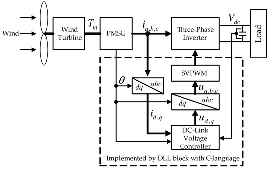
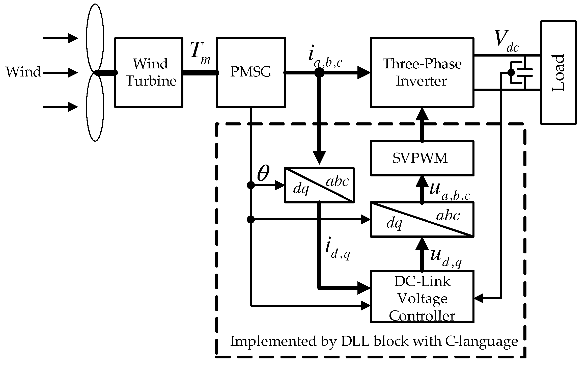
which were used for constructing the control algorithm. The wind turbine part was emulated by adopting the wind turbine block of the renewable energy package in the PSIM software with the nominal output power of 10 kW, a moment of inertia of 1 × ${10}^{-3}$ kg · m², a base wind speed of 20 m/s, a base rotational speed of 50 rpm, and an initial rotational speed of 10 rpm. It was assumed that the wind came from the Weibull distribution-based wind model [24]. The control and the pulse-width modulation (PWM) period were set to be 0.1 ms. Figure 2 depicts the implemented closed-loop system, for which the load-side converter system with an AC load was assumed to be a single-phase passive load for convenience.

Figure 2. The implementation of the closed-loop system

The cut-off frequencies were adjusted as $f_{cc}$ = 200 Hz and $f_{vc}$ = 5 Hz so that

$${\omega }_{cc}=2\pi f_{cc}=1256\mathrm{rad}/\mathrm{s},{\omega }_{vc}=2\pi f_{vc}=31.4\mathrm{rad}/\mathrm{s},$$

which was applied to both of the proposed and feedback linearizing methods. The DOB gains were selected as $l_v=l_d=l_q=314$ rad/s, for the cut-off frequency of the corresponding transfer functions of Equation (34). Note that the d-axis current reference of $i_{d,ref}\left(t\right)$ was set to zero for the maximum torque per ampere (MTPA) operation of the surface-mounted-type PMSG used in this simulation. The decay ratios of the DC-link voltage tracking error and the d-q axis current tracking errors were tuned to be ${\lambda }_{vc}=125.6$ and ${\lambda }_{cc}={\omega }_{cc}=1256$.

The FL technique in [23] used for a comparison is described by

$$\begin{array}{ccc}\hfill u_d\left(t\right)& =& L_{d,0}{\omega }_{cc}{\tilde{i}}_d\left(t\right)+R_{s,0}{\omega }_{cc}{\int }_0^t{\tilde{i}}_d\left(\tau \right)d\tau -L_{q,0}{\omega }_r\left(t\right)i_q\left(t\right)\hfill \end{array}$$

(37)

$$\begin{array}{ccc}\hfill u_q\left(t\right)& =& L_{q,0}{\omega }_{cc}{\tilde{i}}_q\left(t\right)+R_{s,0}{\omega }_{cc}{\int }_0^t{\tilde{i}}_q\left(\tau \right)d\tau +L_{d,0}{\omega }_r\left(t\right)i_d\left(t\right)\hfill \\ & & +{\lambda }_{PM,0}{\omega }_r\left(t\right),\forall t\ge 0\hfill \end{array}$$

(38)

Here, the q-axis current reference comes from

$$\begin{array}{c}\hfill i_{q,ref}\left(t\right)=\frac{v_{dc}\left(t\right)}{b\omega \left(t\right)}\left(2C_0{\omega }_{vc}{\tilde{v}}_{dc}\left(t\right)+C_0{\omega }_{vc}^2{\int }_0^t{\tilde{v}}_{dc}\left(\tau \right)d\tau \right),\forall t\ge 0\end{array}$$

(39)

where ${\tilde{v}}_{dc}\left(t\right)=v_{dc,ref}\left(t\right)-v_{dc}\left(t\right)$, $\forall t\ge 0$. Note that it is easy to verify that the FL method of Equations (37)–(39) approximately yields the current and DC-link voltage-loop transfer functions given by

$$\begin{array}{c}\hfill G_x\left(s\right)=\frac{{\omega }_{cc}}{s+{\omega }_{cc}},x=d,q,G_v\left(s\right)=\frac{{\omega }_{vc}}{s+{\omega }_{vc}},\forall s\in \mathbb{C}\end{array}$$

through the pole-zero cancellation, provided that the nominal parameters are equal to the true parameters, that is, $R_{s,0}=R_s$, $L_{x,0}=L_x$, ${\lambda }_{PM,0}={\lambda }_{PM}$ and $C_0=C$, $x=d,q$. The cut-off frequencies ${\omega }_{cc}$ and ${\omega }_{vc}$ were selected to be the same as for the proposed method.

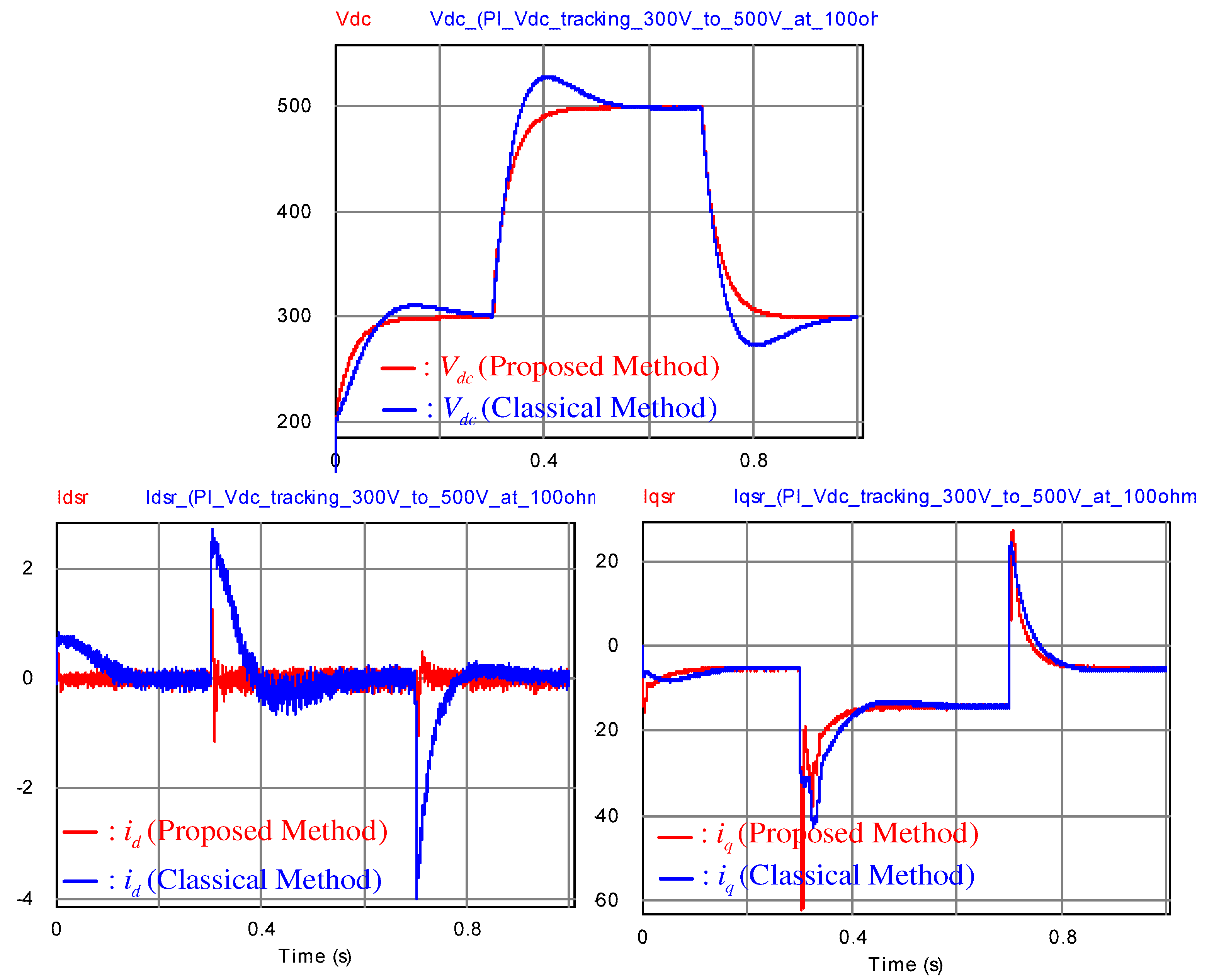
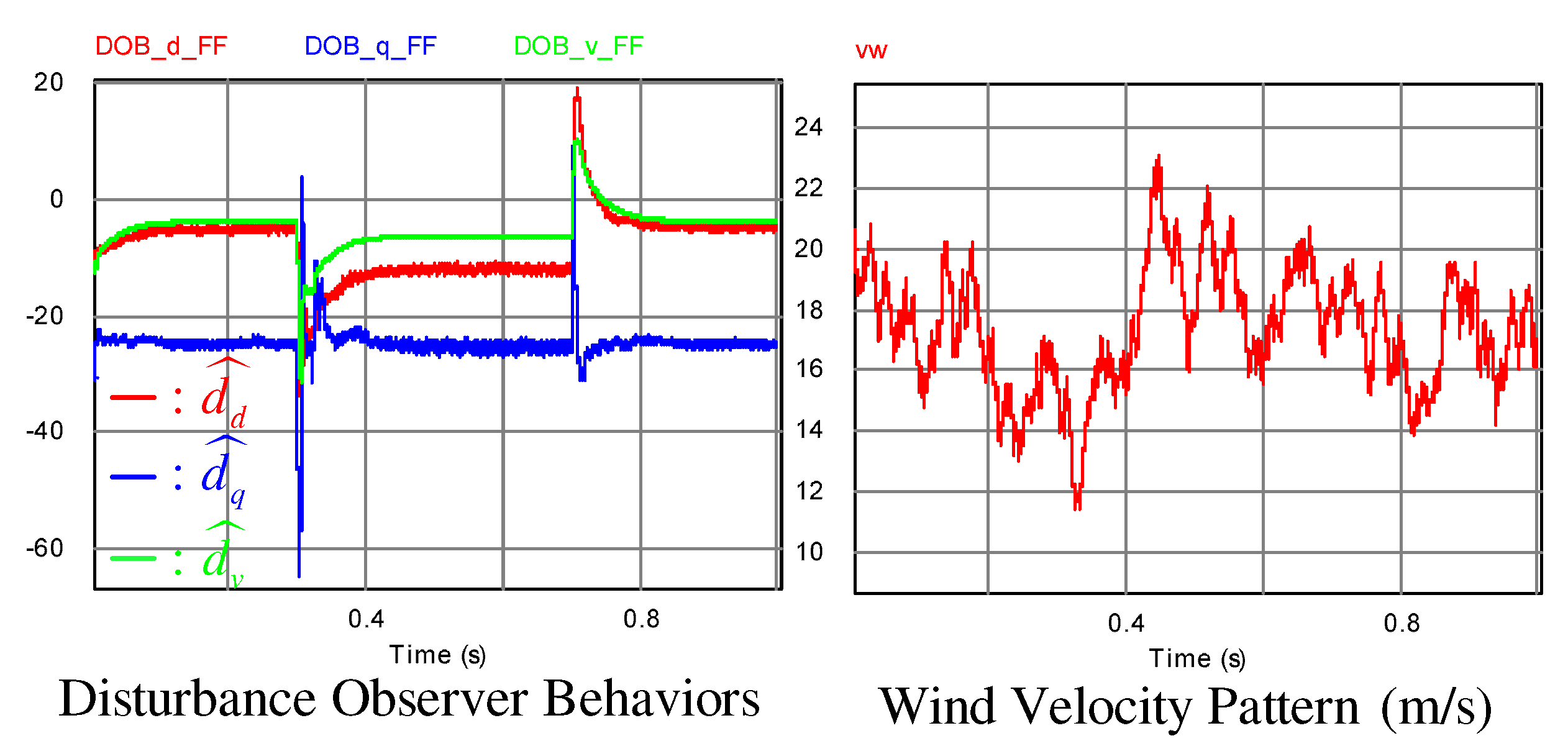
The first simulation was conducted to evaluate the DC-link voltage tracking performance with a resistive load of $R_L=100\Omega$; the DC-link voltage reference was increased from 300 to 500 V, and it was then decreased to 300 V. The simulation results are depicted in Figure 3, and they imply that the proposed method successfully drives the DC-link voltage to rapidly follow its target dynamics of Equation (11) in the presence of the model-plant mismatches. The behaviors of the estimated disturbances and the wind pattern used in this simulation are presented in Figure 4.

Figure 3. The closed-loop performance comparison between the proposed method and the feedback linearizing (FL) method with a resistive load of $R_L=100\Omega$.

Figure 4. The estimated disturbance behaviors and the wind pattern based on the Weibull distribution.

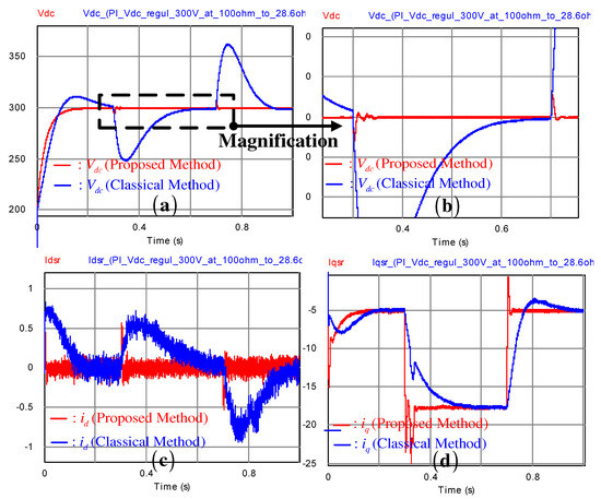
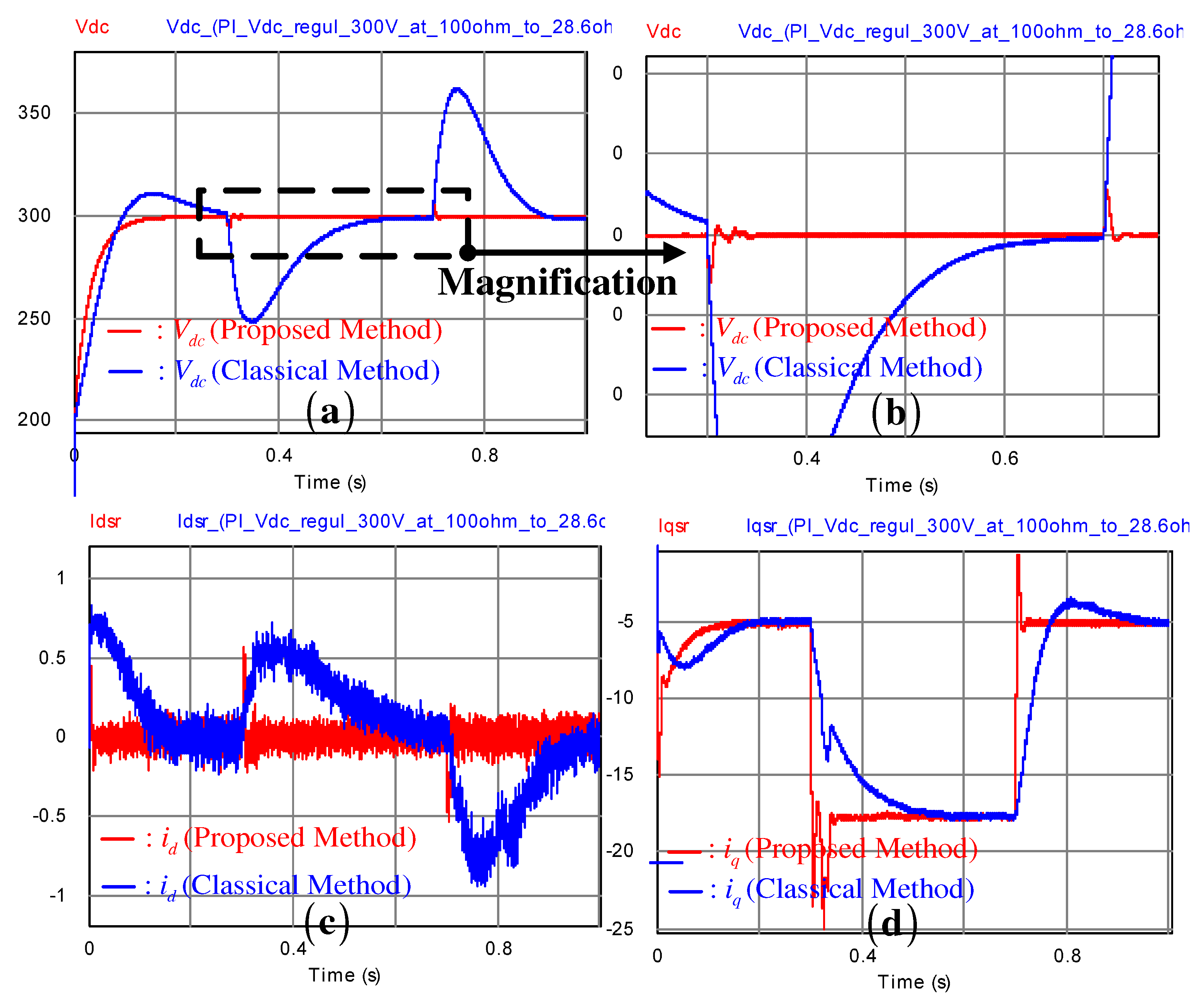
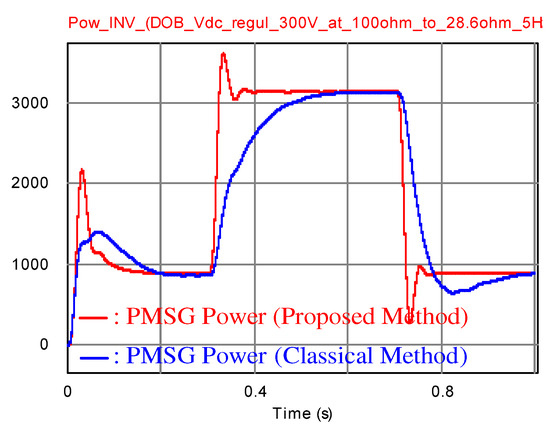
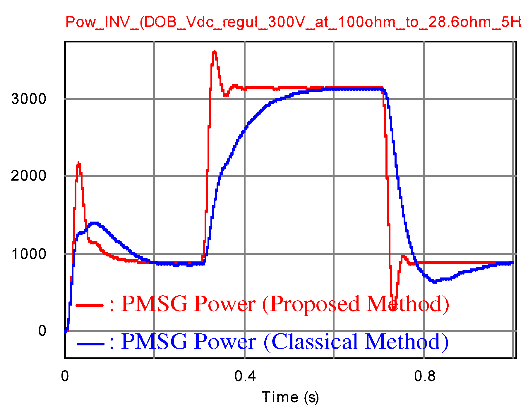
The second simulation compared the DC-link voltage regulation performances by applying the pulse resistive load from $R_L=100\Omega$ to $R_L=28.6\Omega$ at the 300 V operation mode. Figure 5 depicts the comparison results, which imply that the proposed method considerably reduces the over/under shoots caused by the load variations, compared to the classical FL method. The correponding PMSG output power behaviors are presented in Figure 6.

Figure 5. The comparison result of DC-link voltage regulation performance between the proposed method and the feedback linearizing (FL) method at the DC-link voltage of 300 V with a pulse resistive load torque from $R_L=100\Omega$ to $R_L=28.6\Omega$; (a) the resulting output voltage wave forms, (b) a magnified version of (a), (c) d-axis current wave forms, (d) q-axis current wave forms

Figure 6. The permanent magnet synchronous generator (PMSG) output power behaviors of the proposed method and the feedback linearizing (FL) method at the DC-link voltage of 300 V with a pulse resistive load torque from $R_L=100\Omega$ to $R_L=28.6\Omega$.

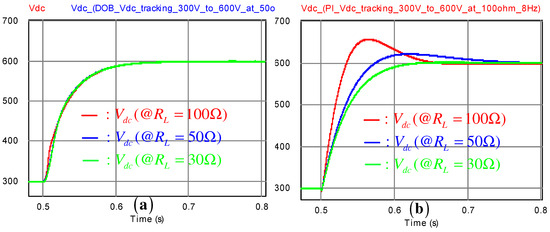
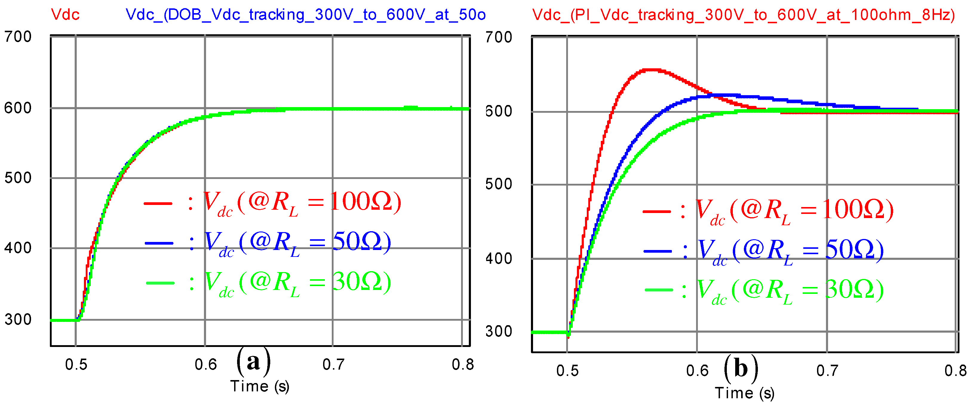
The third simulation was performed to show the closed-loop robustness by investigating the DC-link voltage tracking performance variations for different load conditions, such as $R_L=100,50,30\Omega$. The DC-link voltage reference was increased from 300 to 600 V. The corresponding result is given in Figure 7, which indicates that the proposed method effectively suppresses the DC-link voltage tracking performance variations for several load conditions.

Figure 7. The DC-link voltage tracking performance variation comparison between the proposed method (a) and the feedback linearizing (FL) method (b) at three resistive loads: $R_L=100,50,30\Omega$.

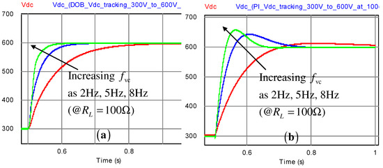
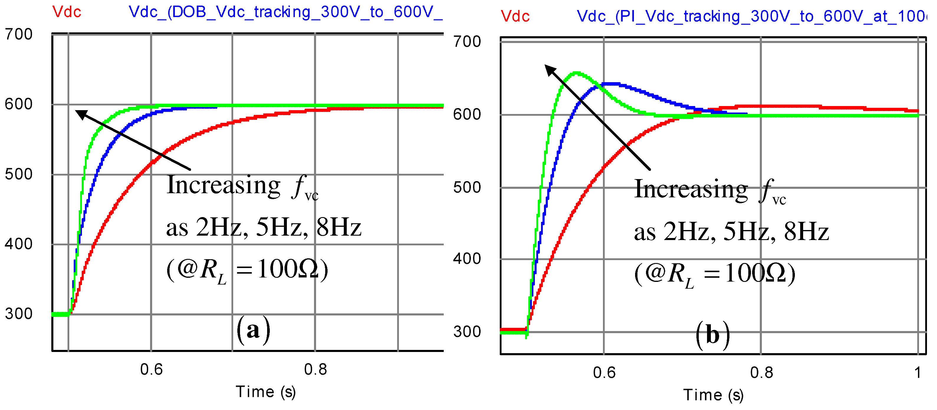
In the last simulation, the DC-link voltage tracking behaviors were compared at a resistive load of $R_L=100\Omega$ with the same DC-link voltage reference by increasing the cut-off frequencies, such as 2, 5, 8 Hz. As can be clearly seen from the result presented in Figure 8, the proposed method efficiently assigns the desired DC-link voltage tracking performance to the closed-loop system, unlike the classical FL technique.

Figure 8. The DC-link voltage tracking behavior comparison between the proposed method (a) and the feedback linearizing (FL) method (b) by increasing the cut-off frequencies, such as 2, 5, 8 Hz.

As shown in the simulation results, in contrast to the classical FL method, the proposed method successfully maintains a satisfactory closed-loop performance despite the operating mode changes. Hence, the proposed method offers almost the same closed-loop performance for various operating ranges without any additional gain scheduling method, which corresponds to a practical advantage of the proposed technique.

5. Conclusions

In this article, a robust DC-link voltage tracking algorithm was proposed by incorporating first-order DOBs in the proportional-type feedback-linearizing DC-link voltage control algorithm. It is rigorously shown that the proposed method guarantees the performance recovery property with the offset-free property. The efficacy of the proposed method has been confirmed by performing realistic simulations for wind power system applications.

References

- Chu, L.; Jia, Y.F.; Chen, D.-S.; Xu, N.; Wang, Y.-W.; Tang, X.; Xu, Z. Research on Control Strategies of an Open-End Winding Permanent Magnet Synchronous Driving Motor (OW-PMSM)-Equipped Dual Inverter with a Switchable Winding Mode for Electric Vehicles. Energies 2017, 10, 616. [Google Scholar] [CrossRef] [Scilit]
- Ding, X.; Du, M.; Cheng, J.; Chen, F.; Ren, S.; Guo, H. Impact of Silicon Carbide Devices on the Dynamic Performance of Permanent Magnet Synchronous Motor Drive Systems for Electric Vehicles. Energies 2017, 10, 364. [Google Scholar] [CrossRef] [Scilit]
- Liu, X.; Du, J.; Liang, D. Analysis and Speed Ripple Mitigation of a Space Vector Pulse Width Modulation-Based Permanent Magnet Synchronous Motor with a Particle Swarm Optimization Algorithm. Energies 2016, 9, 923. [Google Scholar] [CrossRef] [Scilit]
- Yan, H.; Xu, Y.; Zou, J. A Phase Current Reconstruction Approach for Three-Phase Permanent-Magnet Synchronous Motor Drive. Energies 2016, 9, 853. [Google Scholar] [CrossRef] [Scilit]
- Xu, B.; Mu, F.; Shi, G.; Ji, W.; Zhu, H. State Estimation of Permanent Magnet Synchronous Motor Using Improved Square Root UKF. Energies 2016, 9, 489. [Google Scholar] [CrossRef] [Scilit]
- Zhao, J.; Gao, X.; Li, B.; Liu, X.; Guan, X. Open-Phase Fault Tolerance Techniques of Five-Phase Dual-Rotor Permanent Magnet Synchronous Motor. Energies 2015, 8, 12810–12838. [Google Scholar] [CrossRef] [Scilit]
- Dixon, J.W.; Ooi, B.T. Indirect current control of a unity power factor sinusoidal current boost type three phase rectifier. IEEE Trans. Ind. Electron. 1988, 35, 508–515. [Google Scholar] [CrossRef] [Scilit]
- Lee, T.S. Input-output linearization and zero-dynamics control of three-phase AC/DC voltage-source converters. IEEE Trans. Power Electron. 2003, 31, 11–22. [Google Scholar]
- Kazmierkowski, M.P.; Krishnan, R.; Blaabjerg, F. Control in Power Electronics—Selected Problems; Academic Press: Cambridge, MA, USA, 2002. [Google Scholar]
- Lee, T.S. Lagrangian Modeling and Passivity Based Control of Three Phase AC to DC Voltage Source Converters. IEEE Trans. Ind. Electron. 2004, 51, 892–902. [Google Scholar] [CrossRef] [Scilit]
- Bouafia, A.; Gaubert, J.P.; Krim, F. Predictive Direct Power Control of Three-Phase Pulsewidth Modulation (PWM) Rectifier Using Space-Vector Modulation (SVM). IEEE Trans. Power Electron. 2010, 25, 228–236. [Google Scholar] [CrossRef] [Scilit]
- Rodriguez, J.; Cortes, P. Predictive Control of Power Converters and Electrical Drives; Wiley-IEEE Press: Hoboken, NJ, USA, 2012. [Google Scholar]
- Vazquez, S.; Sanchez, J.A.; Carrasco, J.M.; Leon, J.I.; Galvan, E. A model based direct power control for three-phase power converters. IEEE. Trans. Ind. Electron. 2008, 55, 1647–1657. [Google Scholar] [CrossRef] [Scilit]
- De Araujo Ribeiro, R.L.; de Oliveira Alves Rocha, T.; de Sousa, R.M.; dos Santos, E.C.; Lima, A.M.N. A Robust DC-Link Voltage Control Strategy to Enhance the Performance of Shunt Active Power Filters Without Harmonic Detection Schemes. IEEE Trans. Ind. Electron. 2015, 62, 803–813. [Google Scholar] [CrossRef] [Scilit]
- Ge, J.; Zhao, Z.; Yuan, L.; Lu, T.; He, F. Direct Power Control Based on Natural Switching Surface for Three-Phase PWM Rectifiers. IEEE Trans. Power Electron. 2015, 30, 2918–2922. [Google Scholar] [CrossRef] [Scilit]
- Salomonsson, D.; Sannino, A. Direct Power Control Based on Natural Switching Surface for Three-Phase PWM Rectifiers. In Proceedings of the Conference Record of the 2007 IEEE Industry Applications Conference, Forty-Second IAS Annual Meeting, New Orleans, LA, USA, 23–27 September 2007. [Google Scholar]
- Wang, C.; Li, X.; Guo, L.; Li, Y.W. A Nonlinear-Disturbance-Observer-Based DC-Bus Voltage Control for a Hybrid AC/DC Microgrid. IEEE Trans. Power Electron. 2014, 29, 6162–6177. [Google Scholar] [CrossRef] [Scilit]
- Lee, D.C.; Lee, G.M.; Lee, K.D. DC-bus voltage control of three-phase AC/DC PWM converters using feedback linearization. IEEE Trans. Ind. Appl. 2000, 36, 826–833. [Google Scholar]
- Komurcugil, H.; Kukrer, O. Lyapunov-based control for three-phase PWM AC/DC voltage-source converters. IEEE Trans. Power Electron. 1998, 13, 801–813. [Google Scholar] [CrossRef] [Scilit]
- Gomez, M.H.; Ortega, R.; Lagarrigue, F.L.; Escobar, G. Adaptive PI Stabilization of Switched Power Converters. IEEE. Trans. Control Syst. Technol. 2010, 18, 688–698. [Google Scholar] [CrossRef] [Scilit]
- Flores, D.D.P.; Scherpen, J.M.A.; Liserre, M.; de Vries, M.M.J.; Kransse, M.J.; Monopoli, V.G. Passivity-Based Control by Series/Parallel Damping of Single-Phase PWM Voltage Source Converter. IEEE. Trans. Control Syst. Technol. 2012, 3, 459–471. [Google Scholar]
- Krause, P.; Wasynczuk, O.; Sudhoff, S. Analysis of Electric Machinery; IEEE Press: Baltimore, MD, USA, 1995. [Google Scholar]
- Sul, S.K. Control of Electric Machine Drive Systems; Wiley: Hoboken, NJ, USA, 2011; Volume 88. [Google Scholar]
- Mathew, S. Wind Energy: Fundamentals, Resource Analysis and Economics; Springer: Berlin, Germany, 2006. [Google Scholar]
- Khalil, H.K. Nonlinear Systems; Prentice Hall: Upper Saddle River, NJ, USA, 2002. [Google Scholar]
© 2017 by the author. Licensee MDPI, Basel, Switzerland. This article is an open access article distributed under the terms and conditions of the Creative Commons Attribution (CC BY) license (http://creativecommons.org/licenses/by/4.0/).