Article

Enumerative Optimization Procedure for the Gear Train Optimization Problem of a Two-Speed Dedicated Electric Transmission

1
School of Transportation Science and Engineering, Beihang University, 37 Xueyuan Road, Haidian District, Beijing 100191, China
2
Beijing Key Laboratory for High-Efficient Power Transmission and System Control of New Energy Resource Vehicle, Beihang University, 37 Xueyuan Road, Haidian District, Beijing 100191, China
3
DYNAVOLT TECH. and Beihang University Joint Lab for New Energy Resource Vehicle Transmission Technology, Beihang University, 37 Xueyuan Road, Haidian District, Beijing 100191, China
*
Author to whom correspondence should be addressed.
Energies 2017, 10(9), 1362; https://doi.org/10.3390/en10091362
Submission received: 22 July 2017 / Revised: 27 August 2017 / Accepted: 5 September 2017 / Published: 8 September 2017
(This article belongs to the Special Issue Methods to Improve Energy Use in Road Vehicles)

Abstract

:
Gear train optimization problems (GTOPs) can be very difficult. This paper proposes an enumerative optimization procedure (EOP) for the GTOP of a two-speed dedicated electric transmission (2DET) for electric vehicles (EVs). The EOP combines enumeration with the Min-Max Principle of Optimality (MMPO). First, the requirements of the EV and the requirements of manufacture and operation were checked in a dedicated order to obtain the feasible region of the GTOP. Then, the MMPO was implemented within the feasible region to reveal the global optimum in terms of the performance of the EV, the load capacity of the gears and the size of the gear train (GT). Results demonstrated that the EOP was effective in determining the feasible region and simultaneously and globally optimizing multiple criteria for the GTOP. The idea of combining enumeration with optimization, as the EOP presents, may be helpful to solve other GTOPs and provide global optima that are immediately practical and applicable.

1. Introduction

Gear trains (GTs) have been widely used. However, since GTs are quite complex and subjective to design, many GTs are over-designed in terms of the working requirements. Therefore, mainly for better performance or lower cost, gear train optimizations (GTOs) are rather necessary.
Such optimizations are difficult for three main reasons. First, numerous guiding equations, graphs and tables have to be referenced. Second, several key design parameters, for example tooth numbers and moduli, are discrete. Third, some constraints, for example the constraints for bending fatigue and pitting fatigue, are nonlinear. Therefore, although many attempts have been made, GTOs are still developing.
Some GTOs largely depend on algebraic equation derivations or graphical methods. White and Sanger [1] deduced the gear size ratio expressions for a nine-speed GT based on the constraints of mesh conditions and speed ratios. The corresponding graphs of the expressions were used to reveal some typical design points for different optimization purposes. Based on the same constraints, Osman et al. [2] deduced some of the gear size ratio expressions in another way, discovering that only three independent gear size ratios needed to be determined in the nine-speed GTO. Considering more constraints such as that of kinematics and tooth strength, Savage et al. [3] presented feasible design regions graphically for standard involute spur gear sets. They found the optimal designs mainly by analyzing the feasible region graphs. Similarly, Carroll and Johnson [4] formulated a dimensionless optimization model for spur gear sets and then investigated the optima mainly by referencing to dimensionless feasible region graphs. To explore the relationship between problem formulations and solution algorithms, Pomrehn and Papalambros [5] formulated the discrete nonlinear optimization problem for a four-stage spur GT in three equivalent ways, each of which required a different type of algorithms. In a sequel article [6], one of such problem formulations was further reformulated, allowing performing a series of infeasibility and non-optimality tests to significantly reduce the solution space of the problem. However, algebraic equation derivations or graphical methods proposed in those studies [1,2,3,4,5,6] are numerically indirect, which could become rather complex, inefficient and impractical for GTOs when the number of constraints or design variables is large.
Direct numerical methods are demanded for GTOs. Rao and Eslampour [7] presented a two-stage goal programming approach for the multi-objective optimization of multi-stage and multi-speed gearboxes. The kinematic design was first performed and then the strength design. Marjanovic et al. [8] proposed a two-stage optimization procedure for spur GTs. The GT concept was first optimized and then the parameters. Swantner and Campbell [9] proposed a three-stage optimization procedure for GTs consisting of simple, compound, bevel and worm gears. The topology, the gear specifications and the gear locations of the GT, respectively, were optimized at the three stages executed iteratively. However, one part of the whole optimization problem might be dependent on the others to some extent. Therefore, the multi-stage optimization methods for the GTOs in those studies [7,8,9] might lead to local optima, which might be unsatisfying.
To obtain satisfying solutions, some GTOs involve the interaction between the designer and the optimization procedure. Wang and Wang [10] developed an interactive multi-objective design environment for spur gear set optimizations. Huang et al. [11] proposed an interactive physical programming approach for the multi-objective optimization of a three-stage GT. In those studies [10,11], the optimization processes were directed interactively according to the designer’s preferences on design objectives. However, such interactive frameworks [10,11] for GTOs require that the designer should monitor the execution of the optimization program till a satisfying solution is obtained, which might be relatively tiring especially when the running time is long.
To obtain satisfying optima without much manual intervention, random methods are adopted in some GTOs. Zarefar and Muthukrishman [12] developed a modified adaptive random-search algorithm to optimize a helical gear set. Each combination of a starting solution and a search direction, both randomly generated, was tried based on adaptive step sizes to obtain a feasible solution approaching to the constrained boundary, thus iteratively forming a feasible set. Then, the optimum was obtained within the feasible set by direct comparison of objective function values. Thompson et al. [13] presented an optimization tradeoff analysis method for multi-stage spur GTs. The multi-objective problem was formulated as a weighted-sum problem. Systematic variations of all the weightings produced a Pareto optimum set to be plotted and analyzed for discovering the satisfying optimum. Osyczka [14] developed a multi-objective optimization approach based on the Min-Max Principle of Optimality (MMPO) and applied the approach to the automatic design of gearboxes. The solutions for comparison in the min-max sense were randomly generated using the Monte Carlo method or the trade-off studies. Abuid and Ameen [15] proposed a two-stage procedure for accurately minimizing seven criteria of a two-stage spur GT. First, rough optimal solutions were obtained with the random mesh method and the MMPO. Then, to be more accurate, the rough optimal solutions were refined with the direct min-max search method. However, whether the outputs of the random methods in those studies [12,13,14,15] are satisfying greatly depends on the numbers of random trials. Therefore, the efficiencies of those methods might decrease in solving problems of large dimensions for satisfying optima.
In addition, advanced stochastic methods such as the genetic algorithms (GAs), the simulated annealing algorithms (SAAs) and the particle swarm optimization algorithms (PSOAs) are intensively used in some GTOs mainly because these methods can handle various types of design variables, objectives and constraints easily, requiring no information of functional derivatives. Yokota et al. [16] optimized the weight of a gear set with an improved GA. Marcelin [17] proposed a GA combined with a penalty selection method to optimize gear pairs. Mendi et al. [18] used a GA with a static penalty function incorporated in the fitness function to minimize the volume of a single-stage gearbox. Gologlu and Zeyveli [19] utilized a GA to minimize the total volume of a two-stage GT, with static and dynamic penalty function methods implemented to handle constraints. They found that the solutions from the implementation of the dynamic penalty function method were generally better than those from the implementation of the static one. Deb et al. [20] proposed an elitist non-dominated sorting GA to minimize the gear ratio error and the maximum tooth number of a two-stage GT. Deb and Jain [21] implemented the same algorithm to an eighteen-speed gearbox to maximize the power transmitted and minimize the total gear volume. The algorithm generated a set of well-distributed solutions in one single simulation run, providing an opportunity to discover some important design principles. Chong et al. [22] proposed a generalized methodology incorporated an SAA to preliminarily design basic gear parameters and configurations to globally minimize the total volumes of multi-stage GTs. Savsani et al. [23] applied a GA, an SAA and a PSOA to minimize the weight of a spur gear set. The results showed that the PSOA and the SAA were more effective and efficient than the GA. However, numerous trials, especially for inexperienced designers, might have to be performed to appropriately determine several parameters for the advanced stochastic methods used in those studies [16,17,18,19,20,21,22,23] since the efficacies of those methods significantly depend on such parameters. Thus, such a requirement might actually increase the total times for those methods to obtain global optima.
The authors propose an enumerative optimization procedure (EOP) incorporating the MMPO to directly and globally optimize the GT of a two-speed dedicated electric transmission (2DET) for electric vehicles (EVs). The enumeration technique is preferred to the random methods [12,13,14,15] and the advanced stochastic methods [16,17,18,19,20,21,22,23] because the number of the possible solutions to the 2DET could be well limited considering practical manufacturing requirements and a high-performance computer could scan and evaluate all the candidates efficiently. In addition, multiple criteria are simultaneously optimized for the 2DET using the MMPO to find global optima since the MMPO could well represent the real optimization purposes of designers in an intuitive, reasonable and comprehensive way.
The following presents the EOP in detail, illustrated by the GTO of the 2DET. Section 2 introduces the optimization problem of the GT of the 2DET. Section 3 evaluates the constraints in a dedicated order, determining the feasible region of the problem gradually. Section 4 implements the MMPO to the feasible region. Then, the optimization results are displayed and discussed in Section 5. Section 6 concludes the presented work.

2. GT of the 2DET

The GT of the 2DET in this paper is relatively simple (see Figure 1). The GT has six gears, G11, G12, G21, G22, G31 and G32. G11 and G21 can selectively connect to the input shaft, connecting to the motor. G12, G22 and G31 are fixed on the countershaft. G32 is fixed on the differential, connecting to the driving wheels. G11 and G12, G21 and G22, and G31 and G32, respectively, compose G1, G2 and G3, the three gear pairs. G1 and G2 are coaxial. At the neutral gear, the power cannot flow between the input shaft and the differential; at the first gear, the power flows through G1 and G3; and, at the second gear, through G2 and G3.
To appropriately simplify the GTO problem (GTOP) of the 2DET, several assumptions are made. First, all the gears in the 2DET are standard involute gears. Second, the gear working widths of G1, G2 and G3 are respectively 20 mm, 22 mm and 30 mm. Third, the common helical angle of the three gear pairs is 18°. Fourth, the coaxial G1 and G2 share a common gear modulus. Accordingly, the tooth numbers and the moduli of all the six gears are the remaining parameters to basically determine the gears, and are thus chosen to be the design variables. The design variables are constrained by the requirements of the EV (see Table 1) and the requirements of manufacture and operation. The optima of these design variables should be determined by simultaneously optimizing the performance of the EV, the load capacity of the gears and the size of the GT. Although simplified as mentioned above, the GTOP is still quite complicated in terms of the design variables, the constraints and the objectives.

3. Enumeration

Enumeration is direct and practical for determining the feasible regions of the problems with a limited number of possible solutions. The number of the possible solutions of the GTOP is well limited not only because the tooth numbers must be integers and should not be too large or too small but also because the moduli should belong to discrete and limited standard series. Therefore, before the optimal design solutions are obtained, all the candidates are enumerated and evaluated here within the following scopes to determine the feasible region of the GTOP,
{ x 1 , x 2 , x 3 , x 4 , x 5 , x 6 S t o o t h n u m b e r , S t o o t h n u m b e r = { 17 , 18 , , 100 } x 7 S G 1 G 2 m o d u l e , S G 1 G 2 m o d u l e = { 1.25   mm , 1.50   mm , 2.00   mm } x 8 S G 3 m o d u l e , S G 3 m o d u l e = { 2.00   mm , 2.50   mm , 3.00   mm }
where x 1 , x 2 ,…, and x 8 
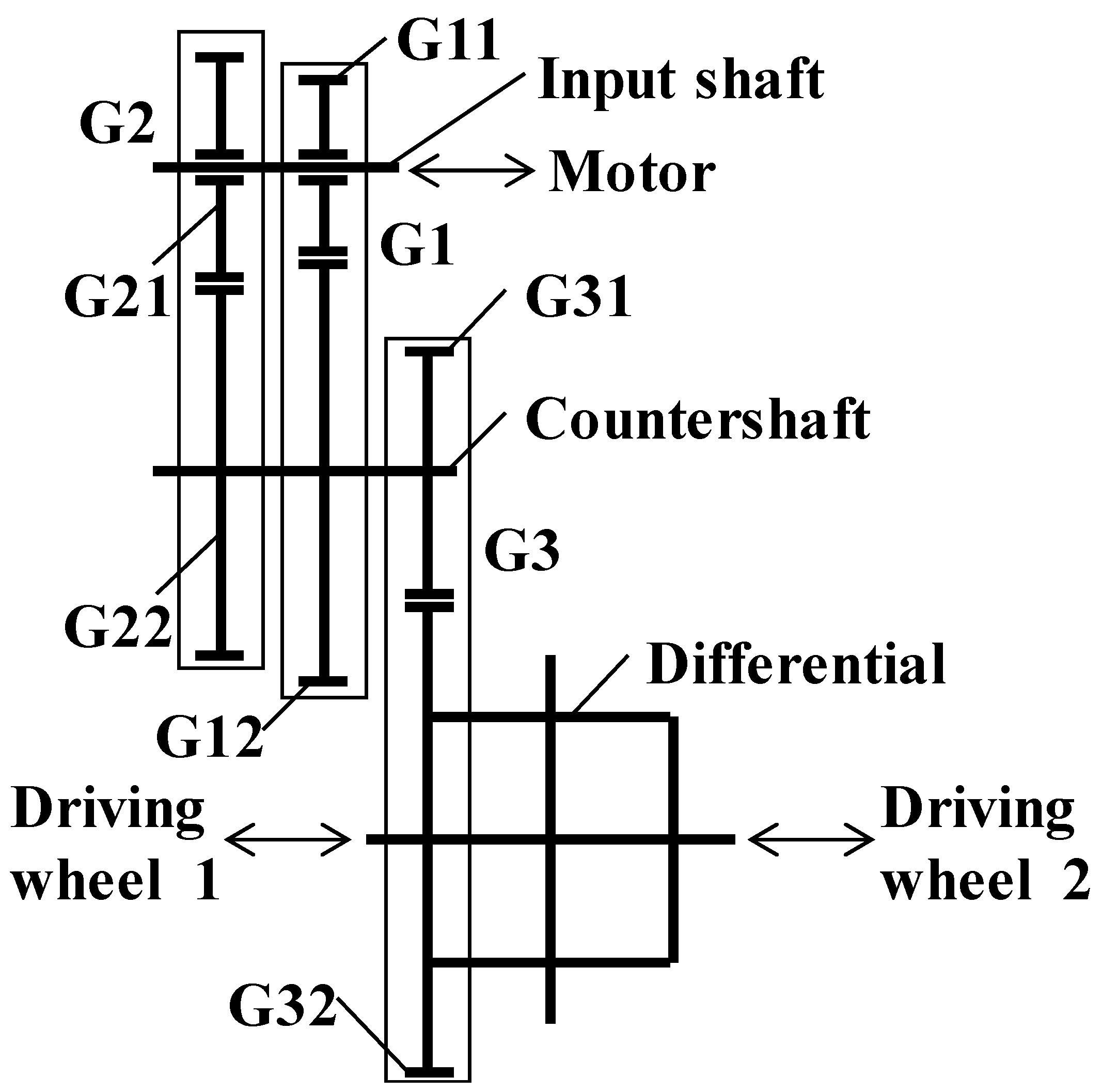
are all the design variables of the GTOP; x 1 , x 2 ,…, and x 6 , respectively, the tooth numbers of G11, G12, G21, G22, G31 and G32; x 7 the common modulus of G1 and G2; x 8 the modulus of G3; S t o o t h n u m b e r the scope of x 1 , x 2 ,…, and x 6 ; and S G 1 G 2 m o d u l e and S G 3 m o d u l e , respectively, the scopes of x 7 and x 8 . Such scopes are established mainly based on engineering experience. According to these scopes, the total number of the possible solutions can be up to
( 100 17 + 1 ) 6 × 3 × 3   =   3.1617 × 10 12
Because of such an enormous quantity of the possible solutions, the evaluation of each possible solution with all the constraints can be impractical. Therefore, the enumeration procedure is elaborated in the following order.

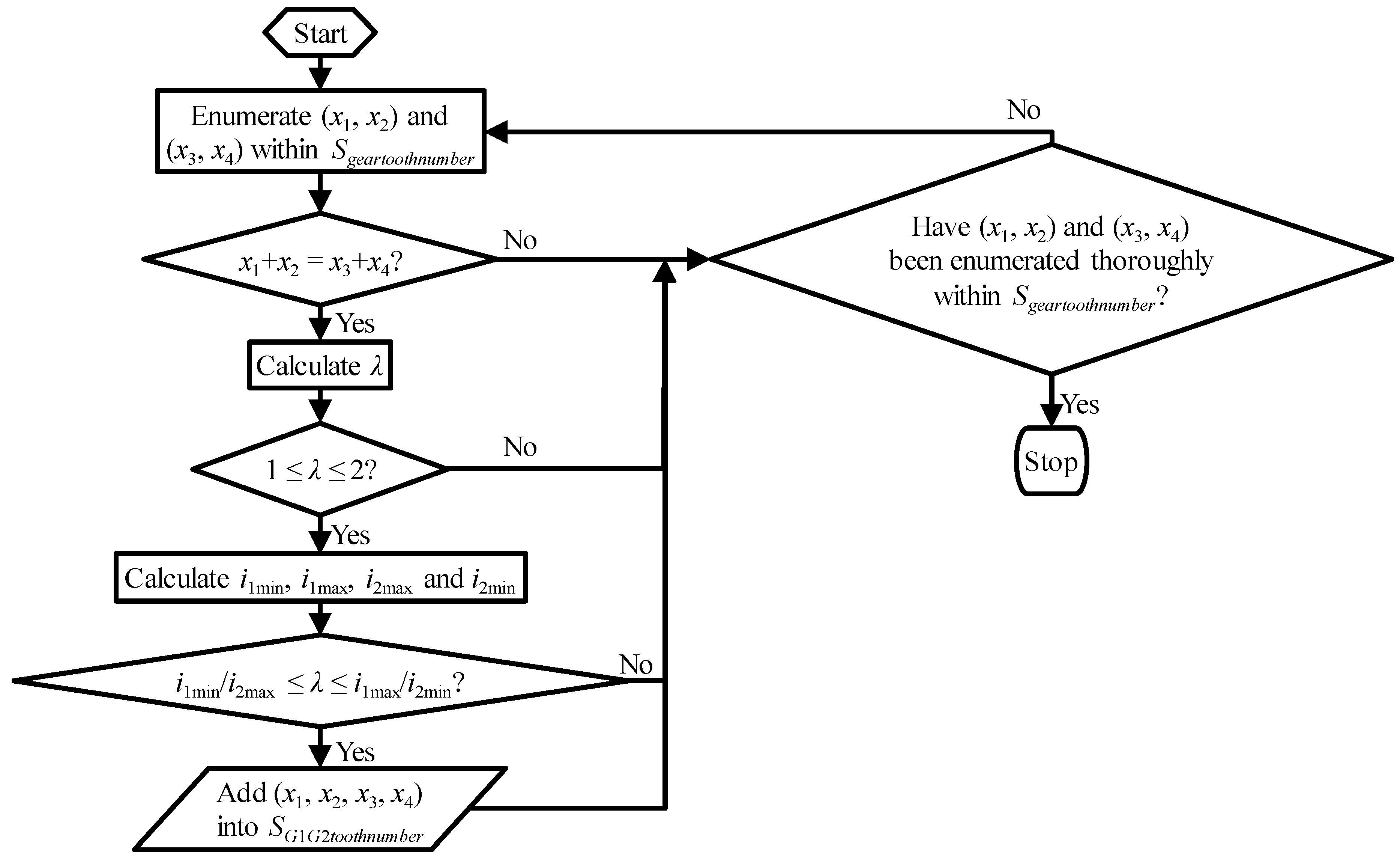
3.1. Tooth Numbers of a Gear Pair

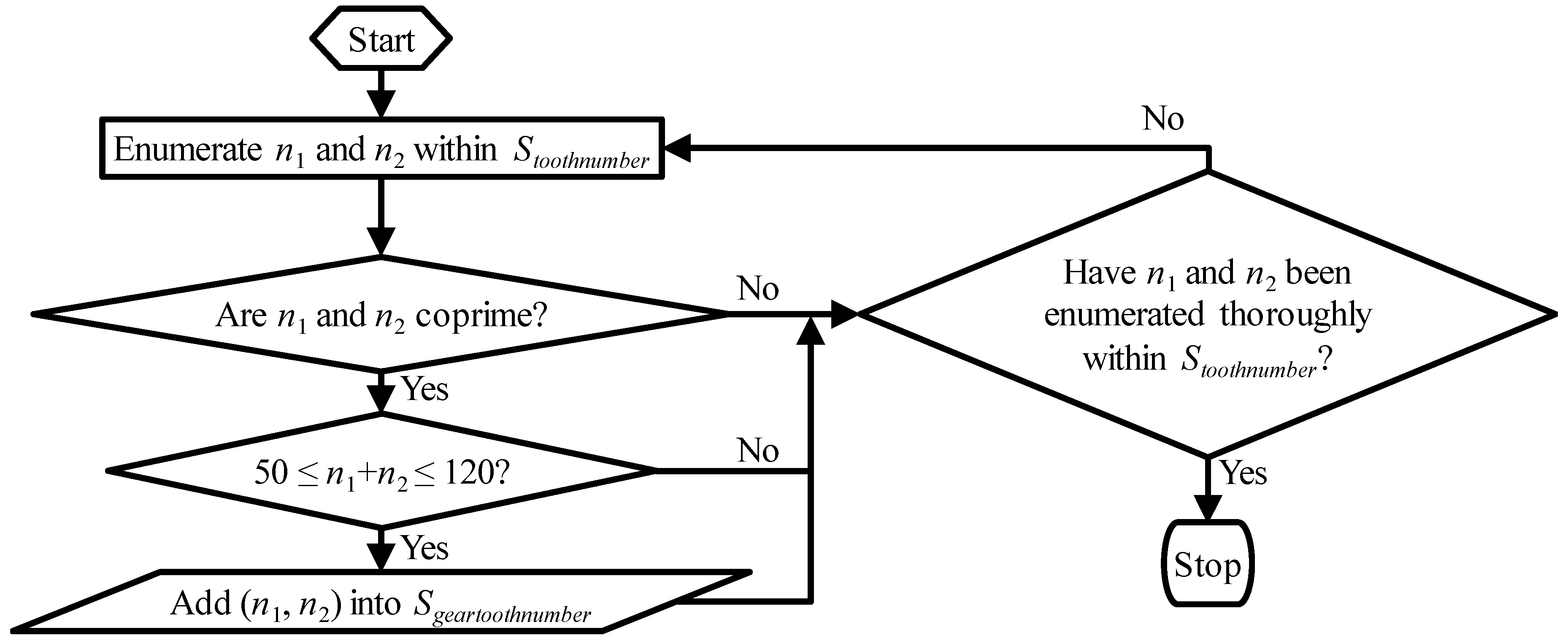
The tooth numbers of a gear pair are preferred to be coprime for the uniform abrasion of the gear pair. Furthermore, the tooth number sum of a gear pair in a vehicle automatic transmission is preferred to be not less than 50 [24] and not larger than 120 [25]. Thus, S g e a r t o o t h n u m b e r , the set of the feasible tooth number combinations of a gear pair, can be expressed as
S g e a r t o o t h n u m b e r = { ( n 1 , n 2 ) | { ( n 1 , n 2 ) = 1 50 n 1 + n 2 120 n 1 , n 2 S t o o t h n u m b e r }
where n 1 and n 2 are the tooth numbers of a gear pair; and ( n 1 , n 2 ) = 1 means n 1 and n 2 are coprime. Figure 2 shows the scheme of the enumeration for the tooth numbers of a gear pair.

3.2. Tooth Numbers of G1 and G2

The following equations show that the gear step ratio λ only depends on the tooth numbers of G1 and G2,
i G 1 = x 2 x 1
i G 2 = x 4 x 3
i G 3 = x 6 x 5
i 1 = i G 1 i G 3 = x 2 x 6 x 1 x 5
i 2 = i G 2 i G 3 = x 4 x 6 x 3 x 5
λ = i 1 i 2 = x 2 x 3 x 1 x 4
where i G 1 , i G 2 and i G 3 are, respectively, the gear ratios of G1, G2 and G3; and i 1 and i 2 , respectively, the first and the second gear ratio. Therefore, the scope of λ can be a constraint for the tooth numbers of G1 and G2. Obviously, i 1 should be greater than i 2 , which means
λ = i 1 i 2 > 1
Besides, usually
λ 2
Furthermore, investigating the scopes of i 1 and i 2 can provide additional lower and upper limits of λ . The climbing ability of the EV requires that
T M max i 1 { [ sgn ( v r a m p ) f cos ( arctan ( θ E V max ) ) + sin ( arctan ( θ E V max ) ) ] m g r o s s g + 0.5 C D ρ A ( v r a m p v a i r ) 2 } r w h e e l
where T M max is the maximum motor torque, sgn (   ) the sign function, v r a m p the vehicle climbing velocity (specified according to GB/T 18385-2005 [26]), f the rolling resistance coefficient, θ E V max the required maximum ramp gradient, m g r o s s the gross mass of the EV, g the acceleration of gravity, C D the air drag coefficient, ρ the air density, A the front area, v a i r the air velocity, and r w h e e l the wheel radius. Therefore, i 1 min , the minimum of i 1 , can be obtained by
i 1 min = { [ sgn ( v r a m p ) f cos ( arctan ( θ E V max ) ) + sin ( arctan ( θ E V max ) ) ] m g r o s s g + 0.5 C D ρ A ( v r a m p v a i r ) 2 } r w h e e l T M max
The adhesion limit of the front-wheel-drive EV requires that
T M max i 1 μ m f r o n t g r w h e e l
where μ is the adhesion coefficient and m f r o n t the front axle laden mass. Therefore, i 1 max , the maximum of i 1 , can be obtained by
i 1 max = μ m f r o n t g r w h e e l T M max
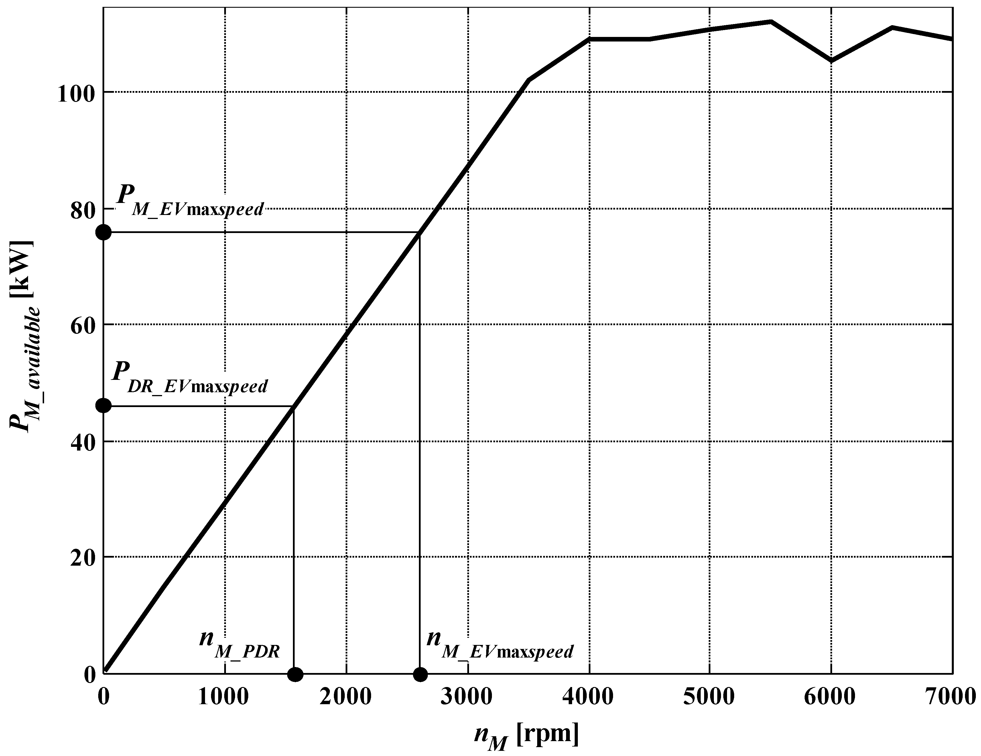
To achieve the required maximum vehicle speed v E V max at the second gear, the following conditions should be met:
n M max r w h e e l i 2 v E V max
P M _ E V max s p e e d P D R _ E V max s p e e d
where n M max is the maximum motor speed, P M _ E V max s p e e d the available motor power at v E V max , and P D R _ E V max s p e e d the driving resistance power of the EV at v E V max . 
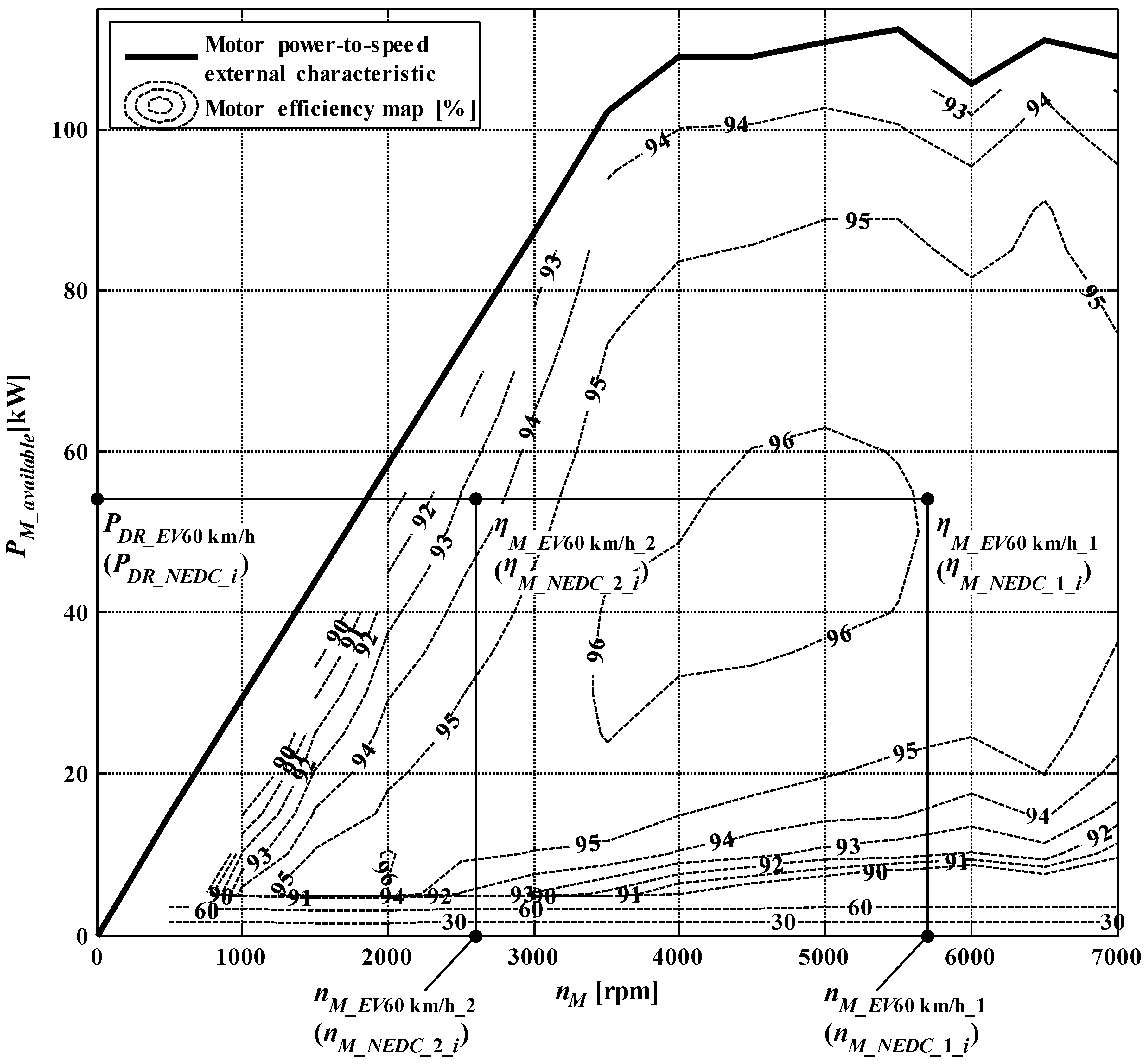
Figure 3 shows the relationship between the available motor power P M _ a v a i l a b l e and the motor speed n M . Based on such relationship,
P M _ a v a i l a b l e = P M _ E V max s p e e d   when   n M = n M _ E V max s p e e d
where n M _ E V max s p e e d is the motor speed corresponding to v E V max and
n M _ E V max s p e e d = i 2 v E V max r w h e e l
P D R _ E V max s p e e d can be calculated by
P D R _ E V max s p e e d = [ sgn ( v E V max ) f m g r o s s g + 0.5 C D ρ A ( v E V max v a i r ) 2 ] v E V max
The motor speed where
P M _ a v a i l a b l e = P D R _ E V max s p e e d
is defined as n M _ P D R and calculated by interpolation. According to Figure 3, Equation (16) leads to
n M _ E V max s p e e d n M _ P D R
Therefore, according to Equations (15), (18) and (21),
i 2 max = n M max r w h e e l v E V max
i 2 min = n M _ P D R r w h e e l v E V max
where i 2 max and i 2 min are, respectively, the maximum and minimum of i 2 .
Thus,
i 1 min i 2 max λ = i 1 i 2 i 1 max i 2 min
Moreover, according to the assumptions made in Section 2, the tooth number sums of G1 and G2 should be the same, which means
x 1 + x 2 = x 3 + x 4
Therefore, S G 1 G 2 t o o t h n u m b e r , the set of feasible tooth number combinations of G1 and G2, can be expressed as
S G 1 G 2 t o o t h n u m b e r = { ( x 1 , x 2 , x 3 , x 4 ) | { 1 < λ 2 i 1 min i 2 max λ i 1 max i 2 min x 1 + x 2 = x 3 + x 4 ( x 1 , x 2 ) , ( x 3 , x 4 ) S g e a r t o o t h n u m b e r }
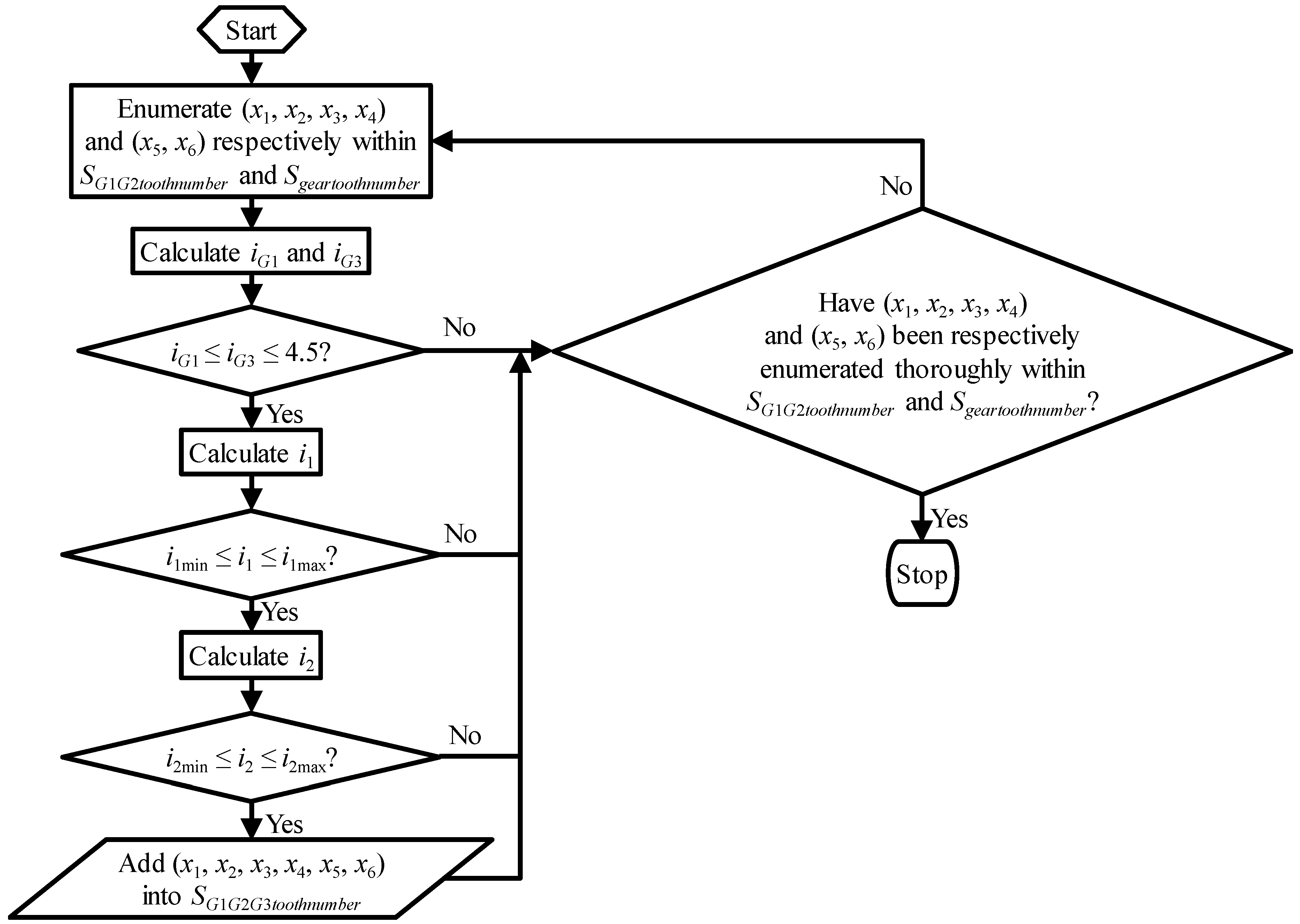
Figure 4 shows the scheme of the enumeration for the tooth numbers of G1 and G2.

3.3. Tooth Numbers of G1, G2 and G3

Engineering experience usually suggests that
i G 1 i G 3 4 . 5
Besides, the scopes of i 1 and i 2 are
i 1 min i 1 i 1 max
i 2 min i 2 i 2 max
Therefore, S G 1 G 2 G 3 t o o t h n u m b e r , the set of feasible tooth number combinations of G1, G2 and G3, can be expressed as
S G 1 G 2 G 3 t o o t h n u m b e r = { ( x 1 , x 2 , x 3 , x 4 , x 5 , x 6 ) | { i G 1 i G 3 4 . 5 i 1 min i 1 i 1 max i 2 min i 2 i 2 max ( x 1 , x 2 , x 3 , x 4 ) S G 1 G 2 t o o t h n u m b e r ( x 5 , x 6 ) S g e a r t o o t h n u m b e r }
Figure 5 shows the scheme of the enumeration for the tooth numbers of G1, G2 and G3.

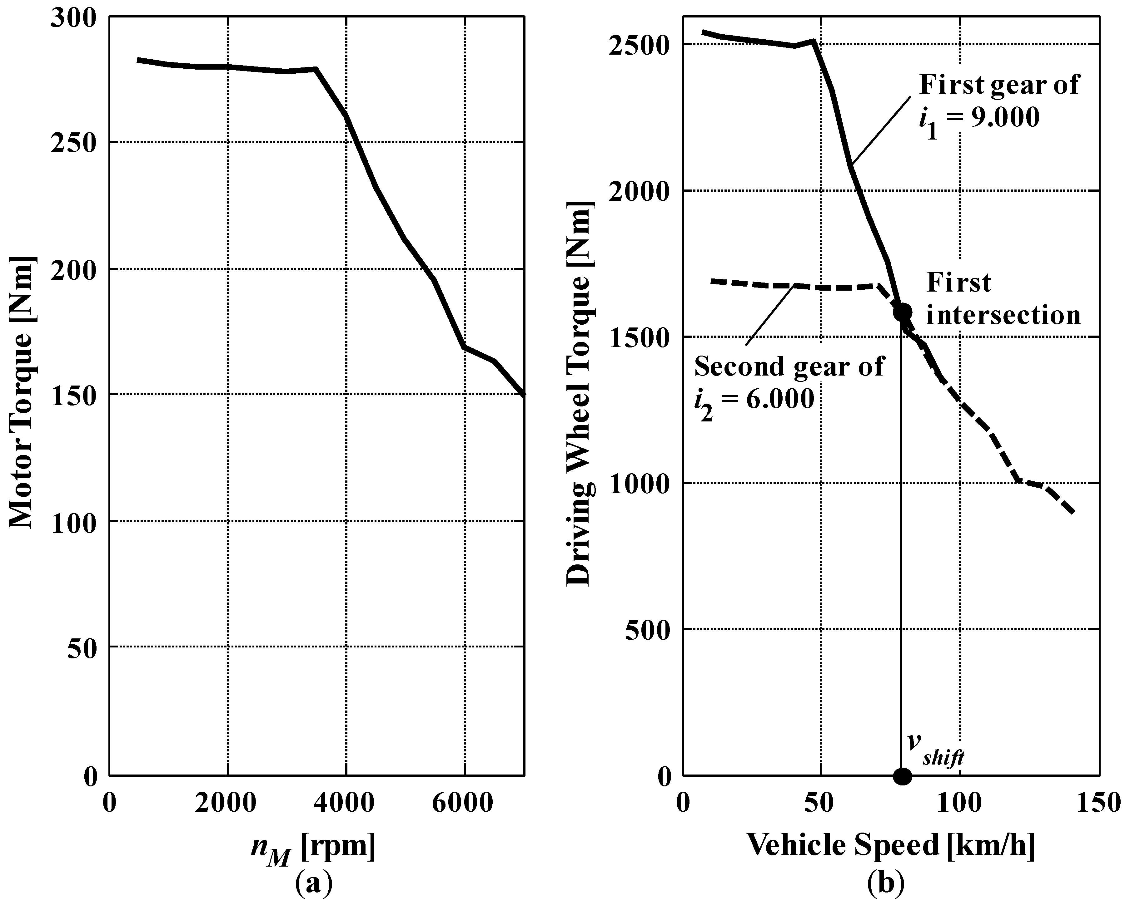
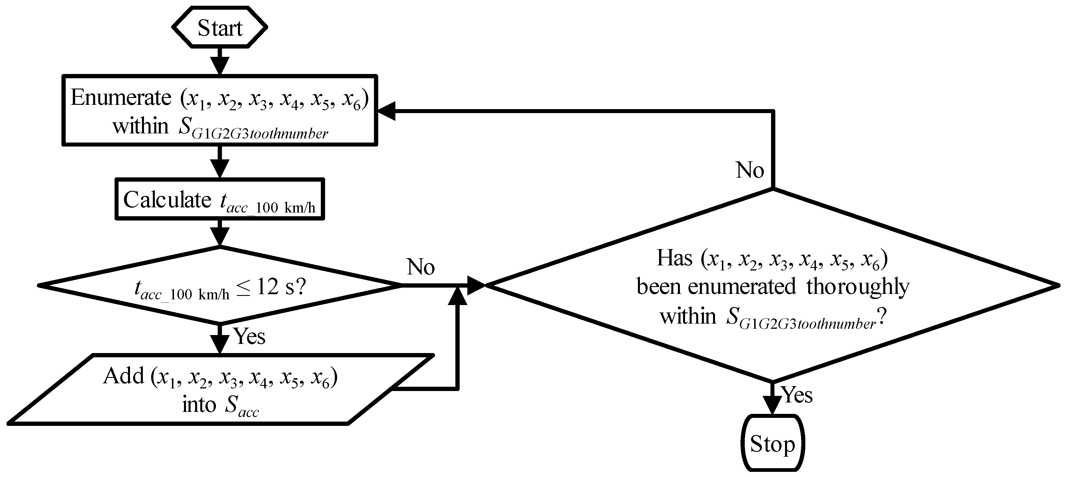
3.4. Acceleration Time

t a c c _ 100   km / h , the 0–100 km/h acceleration time, is a criterion for evaluating the power performance of the EV. For each tooth number combination belonging to S G 1 G 2 G 3 t o o t h n u m b e r , v s h i f t , the shift speed for the 0–100 km/h acceleration test, should be determined before calculating t a c c _ 100   km / h . The motor torque-to-speed external characteristic can be converted into the vehicle torque-to-speed external characteristics of the first and the second gear, based on which v s h i f t is determined. Figure 6 shows an example of the conversion of the characteristics. The first intersection of the two vehicle torque-to-speed curves can be derived with interpolation. The vehicle speed at the intersection is v s h i f t . However, if v s h i f t is larger than v M max s p e e d 1 , the vehicle speed corresponding to n M max at the first gear, then v M max s p e e d 1 is treated as v s h i f t . v M max s p e e d 1 can be obtained by
v M max s p e e d 1 = n M max r w h e e l i 1
The 0–100 km/h acceleration process of the EV is considered in a discrete way. The constant acceleration time step Δ t a c c is 0.1 s. The i -th acceleration time instance t a c c _ i is
t a c c _ i = ( i 1 ) Δ t a c c   ( i = 1 , 2 , 3 , )
The EV speed at t a c c _ i is defined as v a c c _ i , and
v a c c _ i = { 0   km / h   ( i = 1 ) v a c c _ i 1 + a a c c _ i 1 Δ t a c c   ( i = 2 , 3 , 4 , )
where v a c c _ i 1 and a a c c _ i 1 are, respectively, the EV speed and the EV acceleration at the ( i 1 ) -th acceleration time instance t a c c _ i 1 . a a c c _ i 1 can be derived from
a a c c _ i 1 = T w h e e l _ a c c _ i 1 T D R _ a c c _ i 1 r w h e e l m g r o s s   ( i = 2 , 3 , 4 , )
where T w h e e l _ a c c _ i 1 and T D R _ a c c _ i 1 are, respectively, the driving torque and the driving resistance torque at t a c c _ i 1 . T w h e e l _ a c c _ i 1 can be interpolated by v a c c _ i 1 based on the vehicle torque-to-speed external characteristics and v s h i f t . If v a c c _ i 1 is smaller than v s h i f t , the vehicle torque-to-speed external characteristic of the first gear is used to interpolate T w h e e l _ a c c _ i 1 ; otherwise, the vehicle torque-to-speed characteristic of the second gear is used. T D R _ a c c _ i 1 can be obtained using
T D R _ a c c _ i 1 = [ sgn ( v a c c _ i 1 ) f m g r o s s g + 0.5 C D ρ A ( v a c c _ i 1 v a i r ) 2 ] r w h e e l
The first time v a c c _ i reaches 100 km/h, the corresponding acceleration time instance is recorded as t a c c _ 100   km / h .
According to Table 1, t a c c _ 100   km / h should be constrained by
t a c c _ 100   km / h 12   s
Therefore, S a c c , the set of feasible tooth number combinations of G1, G2 and G3 with consideration on the acceleration time, can be expressed as
S a c c = { ( x 1 , x 2 , x 3 , x 4 , x 5 , x 6 ) | { t a c c _ 100   km / h 12   s ( x 1 , x 2 , x 3 , x 4 , x 5 , x 6 ) S G 1 G 2 G 3 t o o t h n u m b e r }
Figure 7 shows the scheme of the enumeration for the acceleration time.

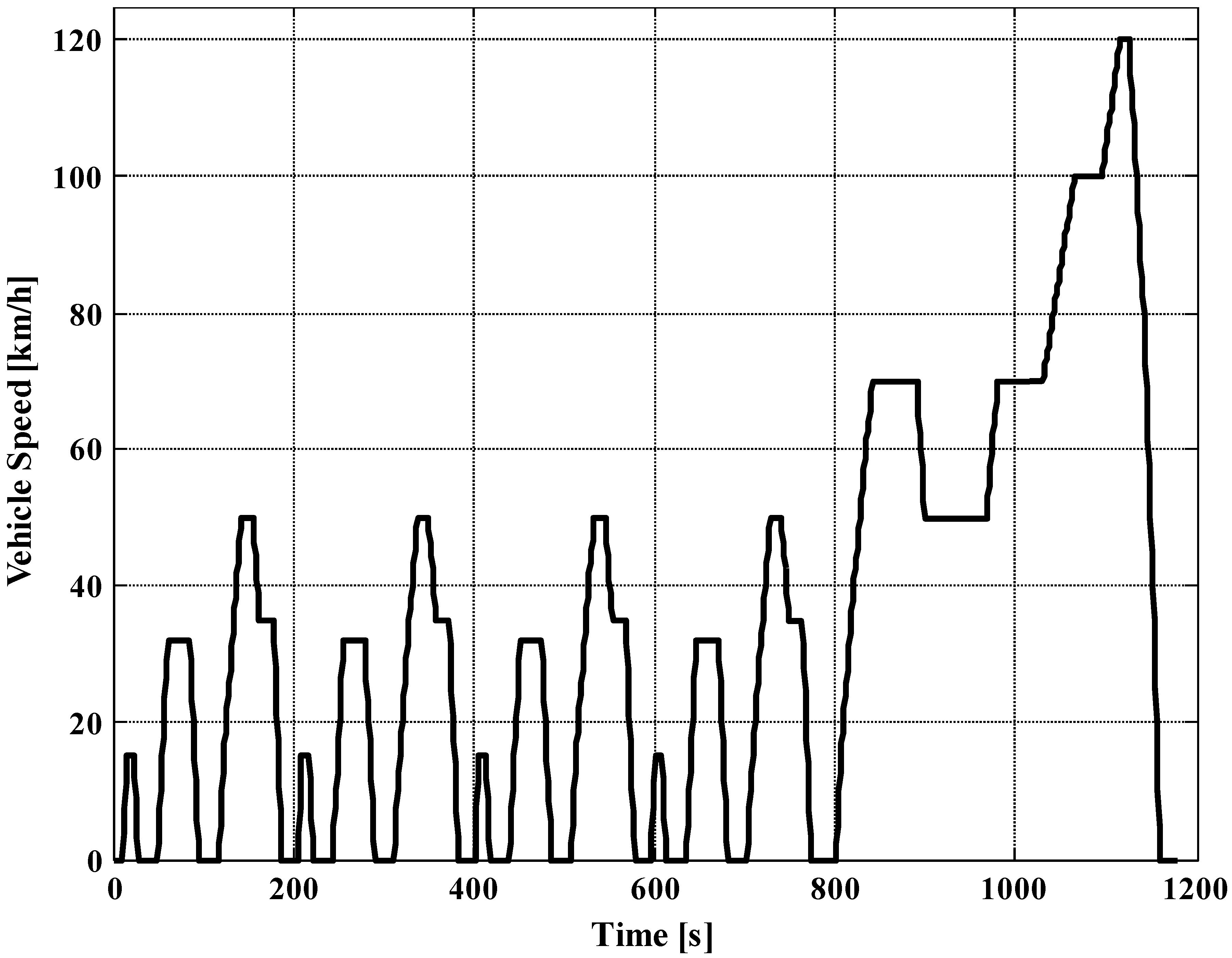
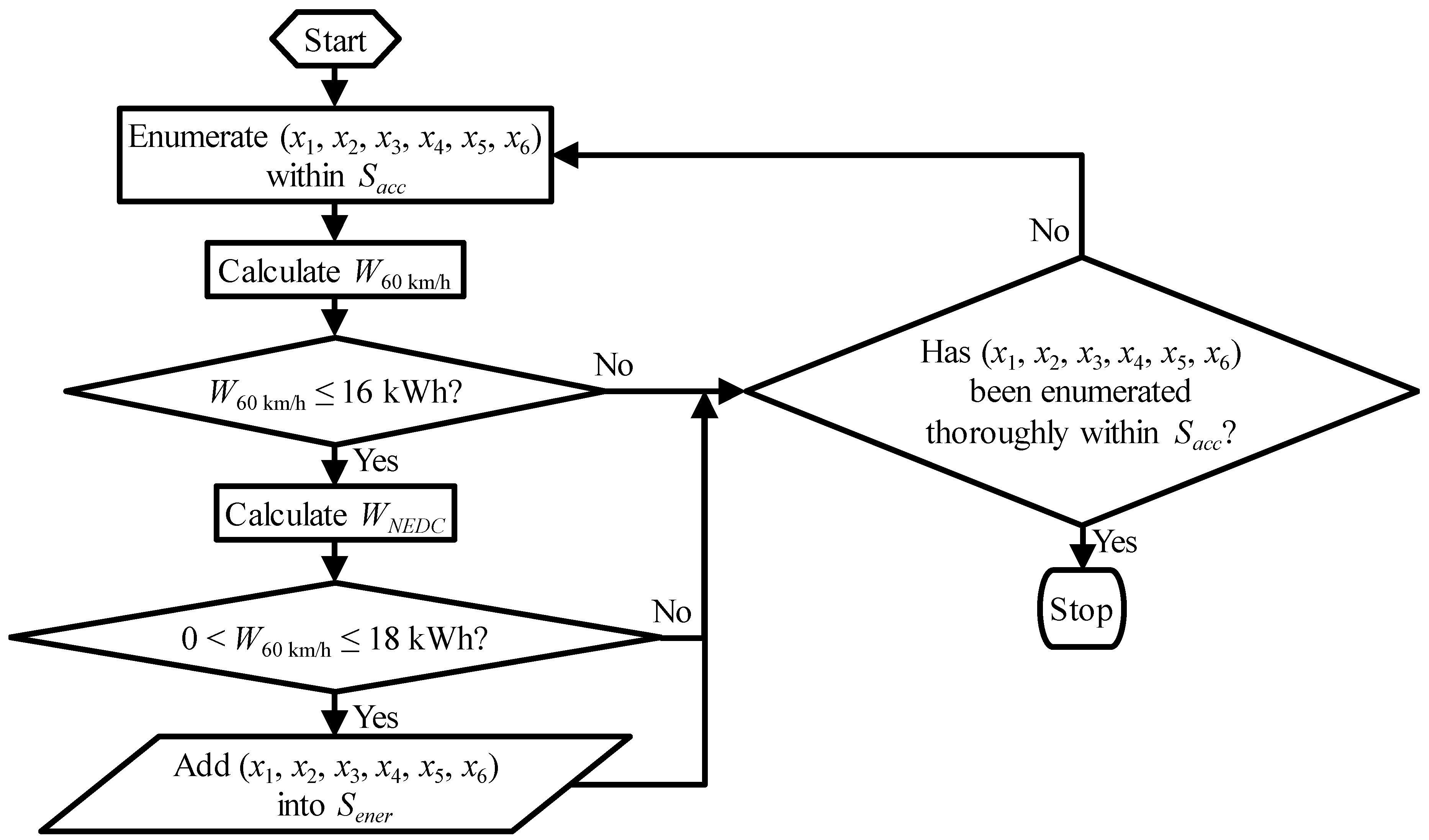
3.5. Energy Consumption

For each element of S a c c , both the 100 km energy consumption at a constant speed of 60 km/h and that according to the New European Driving Cycle (NEDC) [27] (see Figure 8) are criteria for evaluating the economic performance of the EV, respectively, denoted as W 60   km / h and W N E D C . Calculating W 60   km / h and W N E D C requires a knowledge of the efficiency of each power-transition component, such as the battery, the inverter, the motor and the 2DET. For simplification, the efficiencies of all the power-transition components but the motor are assumed to be 100%.
W 60   km / h can be calculated by
W 60   km / h = 100   km 60   km / h P C o n s u m e d _ 60   km / h
where P C o n s u m e d _ 60   km / h is the consumed power of the EV at 60 km/h. P C o n s u m e d _ 60   km / h can be obtained by
P C o n s u m e d _ 60   km / h = P D R _ 60   km / h η M _ 60   km / h
where P D R _ 60   km / h is the driving resistance power of the EV at 60 km/h and η M _ 60   km / h the motor efficiency at 60 km/h. P D R _ 60   km / h can be obtained by
P D R _ 60   km / h = [ f m g r o s s g + 0.5 C D ρ A ( 60   km / h v a i r ) 2 ] 60   km / h
η M _ 60   km / h can be obtained by
η M _ 60   km / h = max ( η M _ 60   km / h _ 1 , η M _ 60   km / h _ 2 )
where η M _ 60   km / h _ 1 and η M _ 60   km / h _ 2 are, respectively, the motor efficiencies of the first and the second gear at 60 km/h. η M _ 60   km / h _ 1 and η M _ 60   km / h _ 2 can be obtained based on the motor efficiency map (see Figure 9) with P D R _ 60   km / h , n M _ 60   km / h _ 1 and n M _ 60   km / h _ 2 , where n M _ 60   km / h _ 1 and n M _ 60   km / h _ 2 are, respectively, the required motor speeds of the first and the second gear at 60 km/h, and
n M _ 60   km / h _ 1 = 60   km / h i 1 r w h e e l
n M _ 60   km / h _ 2 = 60   km / h i 2 r w h e e l
W N E D C can be obtained by
W N E D C = i = 1 i e n d 0.5 ( P C o n s u m e d _ N E D C _ i + P C o n s u m e d _ N E D C _ i + 1 ) Δ t N E D C
where i e n d is the index meaning that, at the ( i e n d + 1 ) -th NEDC time instance t N E D C _ i e n d + 1 , the driving distance first reaches 100 km; P C o n s u m e d _ N E D C _ i and P C o n s u m e d _ N E D C _ i + 1 , respectively, the consumed powers of the EV at the i -th and the ( i + 1 ) -th NEDC time instance t N E D C _ i and t N E D C _ i + 1 ; and Δ t N E D C the constant NEDC time step of 1 s. i e n d is determined by the following equation system
{ i = 1 i e n d 1 0.5 ( v N E D C _ i + v N E D C _ i + 1 ) Δ t N E D C < 100   km i = 1 i e n d 0.5 ( v N E D C _ i + v N E D C _ i + 1 ) Δ t N E D C 100   km
where v N E D C _ i and v N E D C _ i + 1 are, respectively, the EV speeds at t N E D C _ i and t N E D C _ i + 1 . t N E D C _ i can be obtained with
t N E D C _ i = ( i 1 ) Δ t N E D C , i = 1 , 2 , , i e n d + 1
and P C o n s u m e d _ E V N E D C _ i can be obtained with
P C o n s u m e d _ N E D C _ i = { P D R _ N E D C _ i η M _ N E D C _ i if   P D R _ N E D C _ i > 0 P D R _ N E D C _ i η M _ N E D C _ i otherwise
where P D R _ N E D C _ i is the driving resistance power of the EV at t N E D C _ i , and η M _ N E D C _ i the motor efficiency at t N E D C _ i . P D R _ N E D C _ i can be calculated by
P D R _ N E D C _ i = [ sgn ( v N E D C _ i ) f m g r o s s g + 0.5 C D ρ A ( v N E D C _ i v a i r ) 2 + m g r o s s a N E D C _ i ] v N E D C _ i
where a N E D C _ i is the EV acceleration at t N E D C _ i . a N E D C _ i can be calculated by
a N E D C _ i = v N E D C _ i + 1 v N E D C _ i Δ t N E D C
Before determining η M _ N E D C _ i , the working gear at t N E D C _ i should be determined. The required motor speeds of the first and the second gear at t N E D C _ i are, respectively, denoted as n M _ N E D C _ 1 _ i and n M _ N E D C _ 2 _ i , and
n M _ N E D C _ 1 _ i = i 1 v N E D C _ i r w h e e l
n M _ N E D C _ 2 _ i = i 2 v N E D C _ i r w h e e l
Then, η M _ N E D C _ 1 _ i and η M _ N E D C _ 2 _ i , respectively, the motor efficiencies of the first and the second gear at t N E D C _ i , can be obtained based on the motor efficiency map (see Figure 9) with P D R _ N E D C _ i , n M _ N E D C _ 1 _ i and n M _ N E D C _ 2 _ i . In addition, P M _ N E D C _ max _ 1 _ i and P M _ N E D C _ max _ 2 _ i , respectively, the maximum available motor powers of the first and the second gear at t N E D C _ i , can be obtained based on the motor power-to-speed external characteristic (see Figure 3). Symmetrically, P M _ N E D C _ min _ 1 _ i and P M _ N E D C _ min _ 2 _ i , respectively, the minimum available motor powers of the first and the second gear at t N E D C _ i , can be obtained by
P M _ N E D C _ min _ 1 _ i = P M _ N E D C _ max _ 1 _ i
P M _ N E D C _ min _ 2 _ i = P M _ N E D C _ max _ 2 _ i
Besides, T M _ N E D C _ 1 _ i and T M _ N E D C _ 2 _ i , respectively, the required motor torques of the first and the second gear at t N E D C _ i , can be obtained by
T M _ N E D C _ 1 _ i = T D R _ N E D C _ i i 1
where T D R _ N E D C _ i is the driving resistance torque of the EV at t N E D C _ i , and
T D R _ N E D C _ i = [ sgn ( v N E D C _ i ) f m g r o s s g + 0.5 C D ρ A ( v N E D C _ i v a i r ) 2 + m g r o s s a N E D C _ i ] r w h e e l
The following procedure decides the working gear at t N E D C _ i :
Step 1: If
{ v N E D C _ i = 0   km / h v N E D C _ i + 1 = 0   km / h
then the working gear at t N E D C _ i is the neutral gear,
{ n M _ N E D C _ i = 0   rpm T M _ N E D C _ i = 0   Nm η M _ N E D C _ i = 0
where n M _ N E D C _ i and T M _ N E D C _ i are, respectively, the motor speed and the motor torque at t N E D C _ i , and the next step is Step 4. Otherwise, the working gear at t N E D C _ i is not the neutral gear and the next step is Step 2.
Step 2: If
{ n M _ N E D C _ 1 _ i n M max P M _ N E D C _ min _ 1 _ i P D R _ N E D C _ i P M _ N E D C _ max _ 1 _ i η M _ N E D C _ 1 _ i η M _ N E D C _ 2 _ i
then the working gear at t N E D C _ i is the first gear,
{ n M _ N E D C _ i = n M _ N E D C _ 1 _ i T M _ N E D C _ i = T M _ N E D C _ 1 _ i η M _ N E D C _ i = η M _ N E D C _ 1 _ i
and the next step is Step 4. Otherwise, the working gear at t N E D C _ i is not the first gear and the next step is Step 3.
Step 3: If
{ n M _ N E D C _ 2 _ i n M max P M _ N E D C _ min _ 2 _ i P D R _ N E D C _ i P M _ N E D C _ max _ 2 _ i
then the working gear at t N E D C _ i is the second gear,
{ n M _ N E D C _ i = n M _ N E D C _ 2 _ i T M _ N E D C _ i = T M _ N E D C _ 2 _ i η M _ N E D C _ i = η M _ N E D C _ 2 _ i
and the next step is Step 4. Otherwise, the working gear at t N E D C _ i is not the second gear,
W N E D C = 0   kWh
and the calculation of W N E D C for the current element of S a c c stops and that for the next element (if exists) starts.
Step 4: If
{ v N E D C _ i = 0   km / h v N E D C _ i + 1 0   km / h
then t N E D C _ i is a start-up instance for the EV and the next step is Step 5. Otherwise, t N E D C _ i is not a start-up instance for the EV and the next step is Step 6.
Step 5: If
T M _ N E D C _ 1 _ i T M _ s t a r t u p _ max
where T M _ s t a r t u p _ max is the maximum motor start-up torque, then the motor start-up torque demand at t N E D C _ i can be met and the next step is Step 6. Otherwise, the motor start-up torque demand at t N E D C _ i cannot be met,
W N E D C = 0   kWh
and the calculation of W N E D C for the current element of S a c c stops and that for the next element (if exists) starts.
Step 6: The procedure of deciding the working gear at t N E D C _ i ends.
According to Table 1, the energy consumptions of the EV should be constrained by
{ W 60   km / h 16   kWh 0 < W N E D C 18   kWh
Therefore, S e n e r , the set of feasible tooth number combinations of G1, G2 and G3 with consideration on the energy consumption, can be expressed as
S e n e r = { ( x 1 , x 2 , x 3 , x 4 , x 5 , x 6 ) | { W 60   km / h 16   kWh 0 < W N E D C 18   kWh ( x 1 , x 2 , x 3 , x 4 , x 5 , x 6 ) S a c c }
Figure 10 shows the scheme of the enumeration for the energy consumptions.
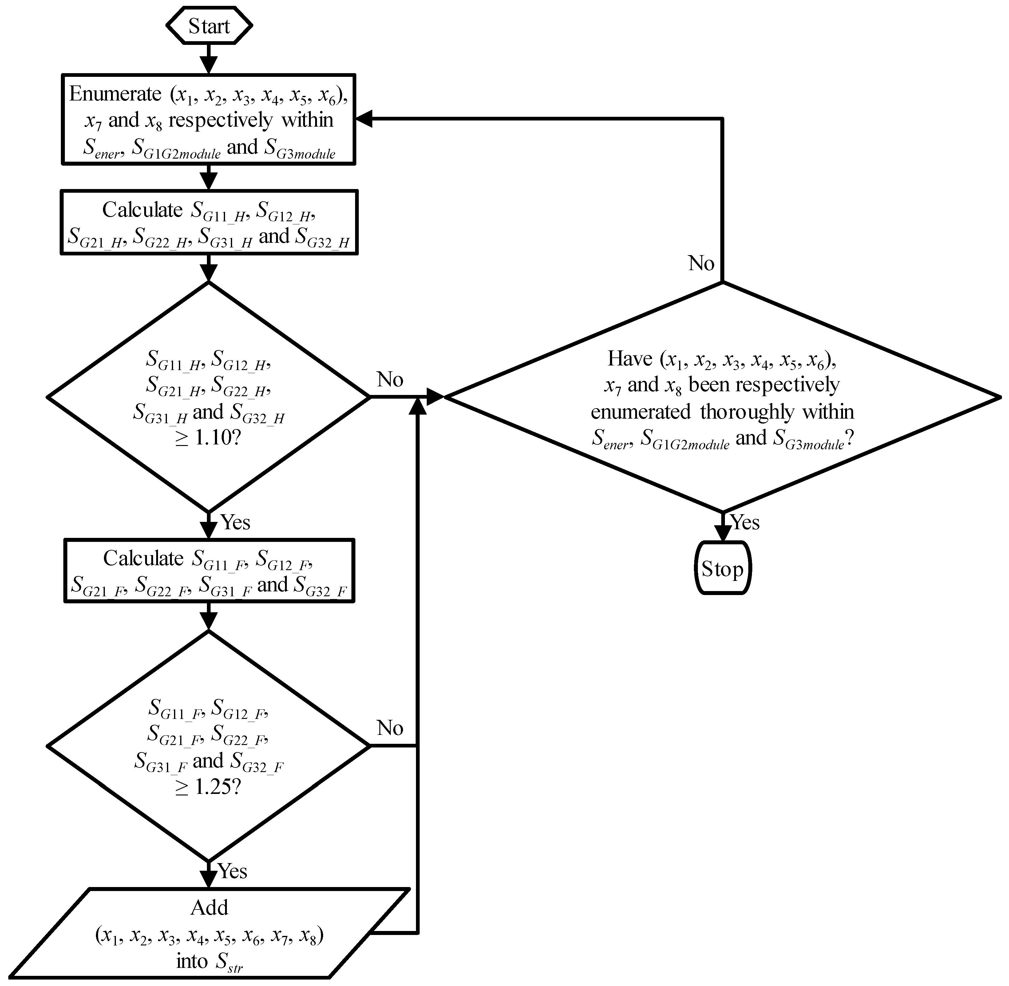
3.6. Safety Factor

The strength safety factors of all the six gears are criteria for evaluating the load capacity of the 2DET. The 200,000 km NEDC is used as the operating condition for the fatigue strength check of the 2DET. For each element of S e n e r , along with the calculation of W N E D C , the time history of the G11, the G21 and the G31 speed can be acquired by
n G 11 _ N E D C _ i = i 1 v N E D C _ i r w h e e l = n M _ N E D C _ 1 _ i
n G 21 _ N E D C _ i = i 2 v N E D C _ i r w h e e l = n M _ N E D C _ 2 _ i
n G 31 _ N E D C _ i = i G 3 v N E D C _ i r w h e e l
where n G 11 _ N E D C _ i , n G 21 _ N E D C _ i and n G 31 _ N E D C _ i are, respectively, the G11, the G21 and the G31 speed at t N E D C _ i . Besides, the time history of the G11, the G21 and the G31 torque can be acquired by
T G 11 _ N E D C _ i = { T D R _ N E D C _ i i 1 = T M _ N E D C _ 1 _ i if   the   working   gear   at   t N E D C _ i   is   the   first   gear 0   Nm otherwise
T G 21 _ N E D C _ i = { T D R _ N E D C _ i i 2 = T M _ N E D C _ 2 _ i if   the   working   gear   at   t N E D C _ i   is   the   sec ond   gear 0   Nm otherwise
T G 31 _ N E D C _ i = T D R _ N E D C _ i i G 3
where T G 11 _ N E D C _ i , T G 21 _ N E D C _ i and T G 31 _ N E D C _ i are, respectively, the G11, the G21 and the G31 torque at t N E D C _ i . Based on ISO 6336-6: 2006(E) [28], the equivalent speeds and the equivalent torques of G11, G21 and G31 in the 100 km NEDC are calculated, regarded as the same with those in the 200,000 km NEDC for simplifying the fatigue strength check. Then, for each combination of x 7 and x 8 , the contact safety factors of G11, G12, G21, G22, G31 and G32, respectively, denoted as S G 11 _ H , S G 12 _ H , S G 21 _ H , S G 22 _ H , S G 31 _ H and S G 32 _ H , and the bending safety factors of G11, G12, G21, G22, G31 and G32, respectively, denoted as S G 11 _ F , S G 12 _ F , S G 21 _ F , S G 22 _ F , S G 31 _ F and S G 32 _ F , can be calculated according to GB/T 3480-1997 [29]. These safety factors should be constrained by
{ S G 11 _ H , S G 12 _ H , S G 21 _ H , S G 22 _ H , S G 31 _ H , S G 32 _ H 1.10 S G 11 _ F , S G 12 _ F , S G 21 _ F , S G 22 _ F , S G 31 _ F , S G 32 _ F 1.25
Therefore, S s t r , the set of feasible tooth number and module combinations of G1, G2 and G3 with consideration on the strength, can be expressed as
S s t r = { ( x 1 , x 2 , x 3 , x 4 , x 5 , x 6 , x 7 , x 8 ) | { S G 11 _ H , S G 12 _ H , S G 21 _ H , S G 22 _ H , S G 31 _ H , S G 32 _ H 1.10 S G 11 _ F , S G 12 _ F , S G 21 _ F , S G 22 _ F , S G 31 _ F , S G 32 _ F 1.25 ( x 1 , x 2 , x 3 , x 4 , x 5 , x 6 ) S e n e r x 7 S G 1 G 2 m o d u l e x 8 S G 3 m o d u l e }
Figure 11 shows the scheme of the enumeration for the safety factors.
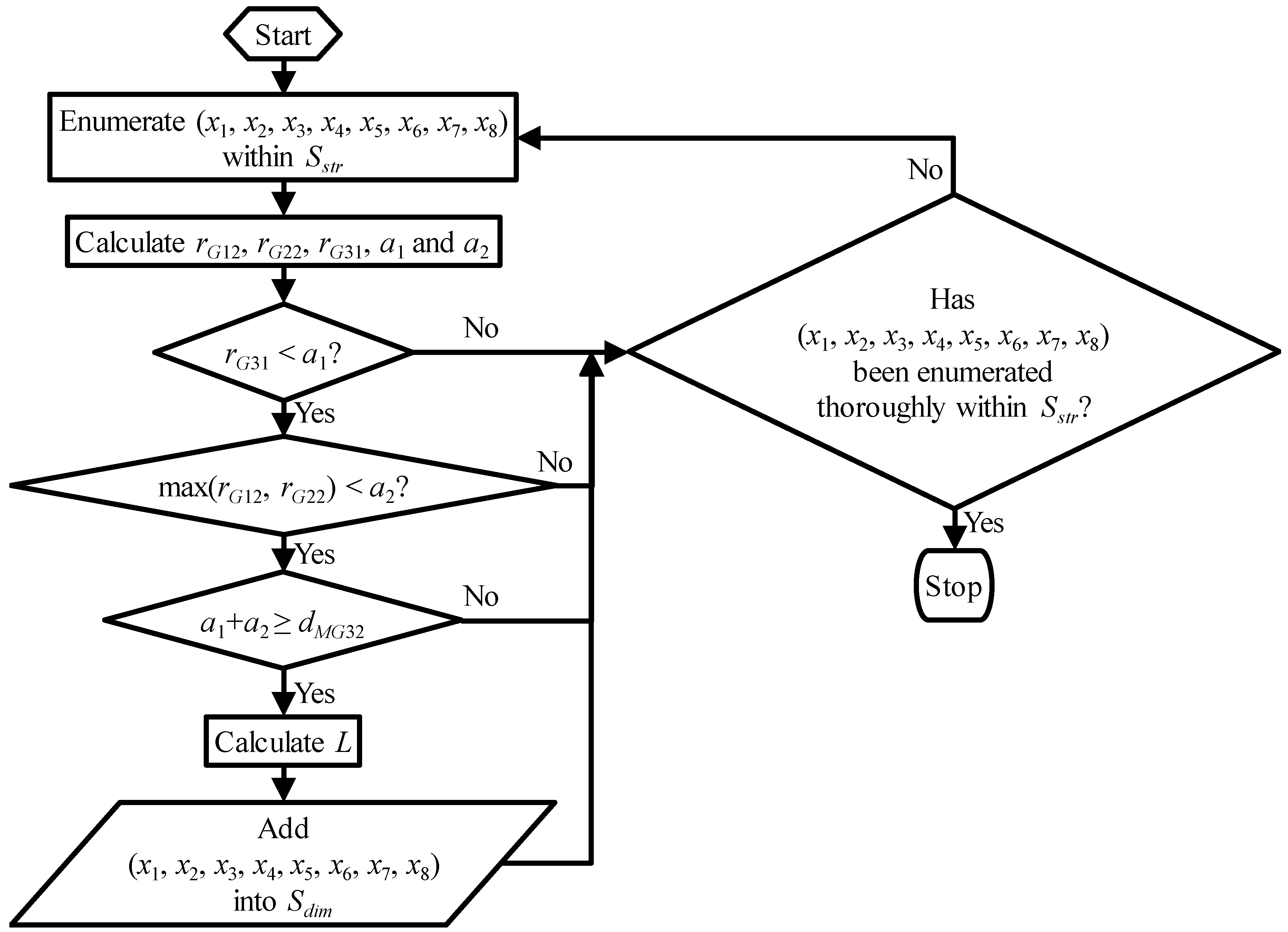
3.7. Dimension

For each element of S s t r , several dimensions can be obtained by
{ r G 11 = x 1 x 7 2 cos 18 ° r G 12 = x 2 x 7 2 cos 18 ° r G 21 = x 3 x 7 2 cos 18 ° r G 22 = x 4 x 7 2 cos 18 ° r G 31 = x 5 x 8 2 cos 18 ° r G 32 = x 6 x 8 2 cos 18 ° a 1 = r G 11 + r G 12 = r G 21 + r G 22 a 2 = r G 31 + r G 32
where r G 11 , r G 12 , r G 21 , r G 22 , r G 31 and r G 32 are, respectively, the reference radii of G11, G12, G21, G22, G31 and G32, and a 1 and a 2 , respectively, the center distances of G1 (or G2) and G3. To avoid interference, the following constraints apply:
r G 31 < a 1
max ( r G 12 , r G 22 ) < a 2
Moreover, the EV arrangement requires that
a 1 + a 2 d M G 32
where d M G 32 is the distance between the rotation axis of the input shaft and that of G32. Therefore, S d i m , the set of feasible tooth number and module combinations of G1, G2 and G3 with consideration on the dimension, can be expressed as
S d i m = { ( x 1 , x 2 , x 3 , x 4 , x 5 , x 6 , x 7 , x 8 ) | { r G 31 < a 1 max ( r G 12 , r G 22 ) < a 2 a 1 + a 2 d M G 32 ( x 1 , x 2 , x 3 , x 4 , x 5 , x 6 , x 7 , x 8 ) S s t r }
For each element of S d i m , the radial length L , representing the size of the GT, can be obtained by
L = a 1 + a 2 + r G 32 + max ( r G 11 , r G 21 )
Figure 12 shows the scheme of the enumeration for the dimensions.

4. MMPO

The optimization method used in this paper is based on the MMPO [14]. According to Osyczka [14], for a multi-criterion optimization problem, the MMPO assumes that none of the criteria change sign and none are equal to zero within the feasible region, and that all the criteria are to be minimized. Based on these assumptions, the fractional increment is defined as [14]
F I i ( X ) = C i ( X ) C i , min 1 0   ( X S , S , i = 1 , 2 , , n , n 2 )
where X is a feasible solution of the multi-criterion optimization problem; S the feasible region of the multi-criterion optimization problem; the empty set; n the number of the criteria, F I i ( X ) and C i ( X ) , respectively, the fractional increment and the value of the i -th criterion of X ; and C i , min the minimum of the i -th criterion. C i , min can be obtained by solving the following single-criterion optimization problem
min f ( X ) = C i ( X ) X S
where f ( X ) is the objective function of the single-criterion optimization problem. F I i ( X ) represents how much C i ( X ) deviates from C i , min . For each X S , F I 1 ( X ) , F I 2 ( X ) ,…, and F I n ( X ) are anew denoted as S F I 1 ( X ) , S F I 2 ( X ) …, and S F I n ( X ) , and
S F I 1 ( X ) S F I 2 ( X ) S F I n ( X )
Using S F I i ( X ) ( i = 1 , 2 , , n ) , the following procedure decides X * , the global optimum of the multi-criterion optimization problem:
Step 1: Set p = 1 , where p is a temporary variable. Solve the following single-criterion optimization problem
min f 1 ( X ) = S F I 1 ( X ) X S
where f 1 ( X ) is the objective function of the single-criterion optimization problem. Denote the set of the optima of the single-criterion optimization problem as S 1 . If only one optimum is obtained, go to Step n + 1 . Otherwise, go to Step 2.
Step 2: Set p = 2 . Solve the following single-criterion optimization problem
min f 2 ( X ) = S F I 2 ( X ) X S 1
where f 2 ( X ) is the objective function of the single-criterion optimization problem. Denote the set of the optima of the single-criterion optimization problem as S 2 . If only one optimum is obtained, go to Step n + 1 . Otherwise, go to Step 3.
Step k ( k 2 ) : Set p = k . Solve the following single-criterion optimization problem
min f k ( X ) = S F I k ( X ) X S k 1
where f k ( X ) is the objective function of the single-criterion optimization problem. Denote the set of the optima of the single-criterion optimization problem as S k . If only one optimum is obtained, go to Step n + 1 . Otherwise, go to Step k + 1 .
Step n : Set p = n . Solve the following single-criterion optimization problem
min f n ( X ) = S F I n ( X ) X S n 1
where f n ( X ) is the objective function of the single-criterion optimization problem. Denote the set of the optima of the single-criterion optimization problem as S n . Go to Step n + 1 .
Step n + 1 : Every element in S p is the global optimum of the multi-criterion optimization problem. The procedure of deciding X * ends.
For a better comprehension of how the MMPO and the fractional increment work, an additional example is presented by Table 2 and Table 3. Table 3 indicates that (0, 0) is the global optimum of the example.
To optimize the GT of the 2DET, the acceleration time t a c c _ 100   km / h , the energy consumptions W 60   km / h and W N E D C , and the radial length L need to be minimized, while the safety factors S G 11 _ H , S G 12 _ H , S G 21 _ H , S G 22 _ H , S G 31 _ H , S G 32 _ H , S G 11 _ F , S G 12 _ F , S G 21 _ F , S G 22 _ F , S G 31 _ F and S G 32 _ F need to be maximized. Since these criteria need to be optimized simultaneously by the MMPO, the maximization problems for the safety factors are converted to the minimization problems for 1 S G 11 _ H , 1 S G 12 _ H , 1 S G 21 _ H , 1 S G 22 _ H , 1 S G 31 _ H , 1 S G 32 _ H , 1 S G 11 _ F , 1 S G 12 _ F , 1 S G 21 _ F , 1 S G 22 _ F , 1 S G 31 _ F and 1 S G 32 _ F .
Due to the limited space, the detail of implementing the MMPO to the GTOP of the 2DET, based on the results from the multi-stage enumeration in Section 3 is not presented.

5. Results and Discussion

The total number of possible solutions can be up to 3 . 1617 × 10 12 . Besides, the preceding text shows that most of the constraints and the objective functions are highly nonlinear and discontinuous, and are difficult to be expressed analytically. However, the number of the elements of S d i m is only 4 . 55306 × 10 5 , sufficiently demonstrating that the multi-stage enumeration is effective in determining the feasible region of the large, non-linear, discontinuous and discrete GTOP of the 2DET.
( x 1 , x 2 , x 3 , x 4 , x 5 , x 6 , x 7 , x 8 ) * , the global optimum of the GTOP of the 2DET, is obtained as
( x 1 , x 2 , x 3 , x 4 , x 5 , x 6 , x 7 , x 8 ) * = ( 23 , 60 , 35 , 48 , 21 , 82 , 2.00   mm , 3.00   mm )
Obviously, the global optimum is directly practical and applicable, requiring little work for further parameterization of the GT of the 2DET.
The minimum and the optimal value of each criterion and the fractional increments of the global optimum are listed in Table 4. Furthermore, the computational process (not displayed) of the MMPO only tackles the objective function of Step 1 but not those of other steps. The optimal value of the objective function of Step 1 is only 0.2758, indicating that the global optimum is quite satisfying and that the MMPO is effective to simultaneously and globally optimize multiple criteria of the same importance.

6. Conclusions

In this paper, a discrete GTOP of a 2DET for an EV was described. Accordingly, an EOP incorporating the MMPO was proposed to solve the GTOP directly and globally. The EOP tackled one type of constraints to reduce the computational load for the next as much as possible, and the sequence of applying the constraints was dedicatedly designed. The constraints consisted of the requirements of manufacture and operation and the requirements of the EV. Resultantly, only 4 . 55306 × 10 5 feasible solutions out of 3 . 1617 × 10 12 possible solutions were reserved for the implementation of the MMPO, sufficiently demonstrating that the EOP is effective in determining the feasible region of the GTOP. The global optimum was quite satisfying in terms of the performance of the EV, the load capacity of the gears and the size of the GT, indicating that the EOP is effective to simultaneously and globally optimize multiple criteria of the same importance.
The idea of combining multi-stage enumeration with optimization, as the EOP shows, may be helpful to optimize the GTs in various applications and provide the global optima which are immediately practical and applicable.

Acknowledgments

This work was supported by the National Natural Science Foundation of China (grant number 51405010) and the National Aerospace Science Foundation of China (grant number 2015ZA51003).

Author Contributions

Xiangyang Xu led the research scheme; Zhifeng Chen investigated relevant research; Zhifeng Chen, Yanjing Liu and Peng Dong designed the EOP; Zhifeng Chen and Yanjing Liu conducted the EOP; Zhifeng Chen and Peng Dong analyzed the data; Zhifeng Chen wrote the paper; and Yanfang Liu checked the whole research.

Conflicts of Interest

The authors declare no conflict of interest. The funding sponsors had no role in the design of the study; in the collection, analyses, or interpretation of data; in the writing of the manuscript, and in the decision to publish the results.

References

  1. White, G.; Sanger, D.J. Design Procedure and Computed Solutions for a Nine-Speed Gear Train Employing Ten Gears. Int. J. Mach. Tool Des. Res. 1968, 8, 141–157. [Google Scholar] [CrossRef]
  2. Osman, M.O.M.; Sankar, S.; Dukkipati, R.V. Design Synthesis of a Multi-Speed Machine Tool Gear Transmission Using Multiparameter Optimization. J. Mech. Des. 1978, 100, 303–310. [Google Scholar] [CrossRef]
  3. Savage, M.; Coy, J.J.; Townsend, D.P. Optimal Tooth Numbers for Compact Standard Spur Gear Sets. J. Mech. Des. 1982, 104, 749–758. [Google Scholar] [CrossRef]
  4. Carroll, R.K.; Johnson, G.E. Dimensionless Solution to the Optimal Design of Spur Gear Sets. J. Mech. Des. 1989, 111, 290–296. [Google Scholar] [CrossRef]
  5. Pomrehn, L.P.; Papalambros, P.Y. Discrete Optimal Design Formulations with Application to Gear Train Design. J. Mech. Des. 1995, 117, 419–424. [Google Scholar] [CrossRef]
  6. Pomrehn, L.P.; Papalambros, P.Y. Infeasibility and Non-Optimality Tests for Solution Space Reduction in Discrete Optimal Design. J. Mech. Des. 1995, 117, 425–432. [Google Scholar] [CrossRef]
  7. Rao, S.S.; Eslampour, H.R. Multistage Multiobjective Optimization of Gearboxes. J. Mech. Transm. Autom. Des. 1986, 108, 461–468. [Google Scholar] [CrossRef]
  8. Marjanovic, N.; Isailovic, B.; Marjanovic, V.; Milojevic, Z.; Blagojevic, M.; Bojic, M. A Practical Approach to the Optimization of Gear Trains with Spur Gears. Mech. Mach. Theory 2012, 53, 1–16. [Google Scholar] [CrossRef]
  9. Swantner, A.; Campbell, M.I. Topological and Parametric Optimization of Gear Trains. Eng. Optim. 2012, 44, 1351–1368. [Google Scholar] [CrossRef]
  10. Wang, H.; Wang, H. Optimal Engineering Design of Spur Gear Sets. Mech. Mach. Theory 1994, 29, 1071–1080. [Google Scholar] [CrossRef]
  11. Huang, H.; Tian, Z.; Zuo, M.J. Multiobjective Optimization of Three-Stage Spur Gear Reduction Units Using Interactive Physical Programming. J. Mech. Sci. Technol. 2005, 19, 1080–1086. [Google Scholar] [CrossRef]
  12. Zarefar, H.; Muthukrishnan, S.N. Computer-Aided Optimal Design via Modified Adaptive Random-Search Algorithm. Comput.-Aided Des. 1993, 25, 240–248. [Google Scholar] [CrossRef]
  13. Thompson, D.F.; Gupta, S.; Shukla, A. Tradeoff Analysis in Minimum Volume Design of Multi-Stage Spur Gear Reduction Units. Mech. Mach. Theory 2000, 35, 609–627. [Google Scholar] [CrossRef]
  14. Osyczka, A. An Approach to Multicriterion Optimization Problems for Engineering Design. Comput. Methods Appl. Mech. Eng. 1978, 15, 309–333. [Google Scholar] [CrossRef]
  15. Abuid, B.A.; Ameen, Y.M. Procedure for Optimum Design of a Two-Stage Spur Gear System. JSME Int. J. Ser. C Mech. Syst. Mach. Elem. Manuf. 2003, 46, 1582–1590. [Google Scholar] [CrossRef]
  16. Yokota, T.; Taguchi, T.; Gen, M. A Solution Method for Optimal Weight Design Problem of the Gear Using Genetic Algorithms. Comput. Ind. Eng. 1998, 35, 523–526. [Google Scholar] [CrossRef]
  17. Marcelin, J.L. Genetic Optimisation of Gears. Int. J. Adv. Manuf. Technol. 2001, 17, 910–915. [Google Scholar] [CrossRef]
  18. Mendi, F.; Başkal, T.; Boran, K.; Boran, F.E. Optimization of Module, Shaft Diameter and Rolling Bearing for Spur Gear through Genetic Algorithm. Expert Syst. Appl. 2010, 37, 8058–8064. [Google Scholar] [CrossRef]
  19. Gologlu, C.; Zeyveli, M. A Genetic Approach to Automate Preliminary Design of Gear Drives. Comput. Ind. Eng. 2009, 57, 1043–1051. [Google Scholar] [CrossRef]
  20. Deb, K.; Pratap, A.; Moitra, S. Mechanical Component Design for Multiple Objectives Using Elitist Non-Dominated Sorting GA. In Proceedings of the International Conference on Parallel Problem Solving from Nature, Paris, France, 18–20 September 2000; Schoenauer, M., Deb, K., Rudolph, G., Yao, X., Lutton, E., Merelo, J.J., Schwefel, H., Eds.; Springer: Berlin, Germany, 2000; pp. 859–868. [Google Scholar]
  21. Deb, K.; Jain, S. Multi-Speed Gearbox Design Using Multi-Objective Evolutionary Algorithms. J. Mech. Des. 2003, 125, 609–619. [Google Scholar] [CrossRef]
  22. Chong, T.H.; Bae, I.; Park, G. A New and Generalized Methodology to Design Multi-Stage Gear Drives by Integrating the Dimensional and the Configuration Design Process. Mech. Mach. Theory 2002, 37, 295–310. [Google Scholar] [CrossRef]
  23. Savsani, V.; Rao, R.V.; Vakharia, D.P. Optimal Weight Design of a Gear Train Using Particle Swarm Optimization and Simulated Annealing Algorithms. Mech. Mach. Theory 2010, 45, 531–541. [Google Scholar] [CrossRef]
  24. Handbook of Automobile Engineering–Design; China Communications Press: Beijing, China, 2001; p. 453. ISBN 7-114-03930-1. (In Chinese)
  25. Handbook of Mechanical Design–Reducers and Transmissions; China Machine Press: Beijing, China, 2007; pp. 255–279. ISBN 978-7-111-20971-3. (In Chinese)
  26. GB/T 18385-2005, Electric Vehicles–Power Performance–Test Method; Standards Press of China: Beijing, China, 2005. (In Chinese)
  27. GB/T 18386-2005, Electric Vehicles–Energy Consumption and Range–Test Procedures; Standards Press of China: Beijing, China, 2005. (In Chinese)
  28. ISO 6336-6: 2006(E), Calculation of Load Capacity of Spur and Helical Gears–Part 6: Calculation of Service Life under Variable Load; ISO: Geneva, Switzerland, 2006.
  29. GB/T 3480-1997, Calculation Methods of Load Capacity for Involute Cylindrical Gears; Standards Press of China: Beijing, China, 1997. (In Chinese)
Figure 1. Gear train (GT) of the two-speed dedicated electric transmission (2DET).
Energies 10 01362 g001
Figure 2. Scheme of the enumeration for the tooth numbers of a gear pair.
Energies 10 01362 g002
Figure 3. Motor power-to-speed external characteristics.
Energies 10 01362 g003
Figure 4. Scheme of the enumeration for the tooth numbers of G1 and G2.
Energies 10 01362 g004
Figure 5. Scheme of the enumeration for the tooth numbers of G1, G2 and G3.
Energies 10 01362 g005
Figure 6. Example of the conversion from the motor torque-to-speed external characteristic to the vehicle torque-to-speed external characteristics: (a) motor torque-to-speed external characteristic; and (b) vehicle torque-to-speed external characteristics of the first and the second gear.
Energies 10 01362 g006
Figure 7. Scheme of the enumeration for the acceleration time.
Energies 10 01362 g007
Figure 8. New European Driving Cycle (NEDC).
Energies 10 01362 g008
Figure 9. Motor efficiency map.
Energies 10 01362 g009
Figure 10. Scheme of the enumeration for the energy consumptions.
Energies 10 01362 g010
Figure 11. Scheme of the enumeration for the safety factors.
Energies 10 01362 g011
Figure 12. Scheme of the enumeration for the dimensions.
Energies 10 01362 g012
Table 1. Parameters and requirements of the electric vehicle (EV).
ParameterValueParameterValue
T M max 270 Nm v r a m p 0.6 km/h
f 0.015 θ E V max 30%
m g r o s s 2256 kg g 9.807 m/s2
C D 0.33 ρ 1.2258 Ns2/m4
A 2.2 m2 v a i r 0 km/h
r w h e e l 0.3216 m μ 0.8
m f r o n t 1139 kg v E V max 150 km/h
n M max 7000 r/min t a c c _ 100   km / h ≤12 s
W 60   km / h ≤16 kWh W N E D C ≤18 kWh
T M _ s t a r t u p _ max 283.8398 Nm d M G 32 214 mm
Table 2. Example of the optimization with the Min-Max Principle of Optimality (MMPO): data preparation.
X ( X S ) C 1 ( X ) C 2 ( X ) F I 1 ( X ) F I 2 ( X ) S F I 1 ( X ) S F I 2 ( X )
(0, 0)1 ( C 1 , min )30220
(0, 1)322121
(1, 0)41 ( C 2 , min )3030
Table 3. Example of the optimization with the MMPO: results of Steps 1 and 2.
X ( X S 1 ) f 1 ( X ) X ( X S 2 ) f 2 ( X )
(0, 0)2(0, 0)0
(0, 1)2--
Table 4. Results of the gear train optimization problem (GTOP) of the two-speed dedicated electric transmission (2DET).
CriterionMinimumOptimal ValueFractional Increment
t a c c _ 100   km / h 10.4 s10.5 s0.0096
W 60   km / h 13.1759 kWh13.4033 kWh0.0173
W N E D C 15.7679 kWh15.7760 kWh0.0005
L 325.9533 mm415.8533 mm0.2758
1 S G 11 _ H 0.30890.38300.2398
1 S G 12 _ H 0.30420.38040.2505
1 S G 21 _ H 0.28200.32850.1648
1 S G 22 _ H 0.28030.32710.1671
1 S G 31 _ H 0.26960.33850.2553
1 S G 32 _ H 0.26540.33680.2690
1 S G 11 _ F 0.14830.18800.2678
1 S G 12 _ F 0.14240.17430.2239
1 S G 21 _ F 0.14180.15890.1202
1 S G 22 _ F 0.13970.15560.1134
1 S G 31 _ F 0.12900.15420.1955
1 S G 32 _ F 0.11770.13960.1861

