Flame Front Propagation in an Optical GDI Engine under Stoichiometric and Lean Burn Conditions

Abstract

Lean fueling of spark ignited (SI) engines is a valid method for increasing efficiency and reducing nitric oxide (NO_x) emissions. Gasoline direct injection (GDI) allows better fuel economy with respect to the port-fuel injection configuration, through greater flexibility to load changes, reduced tendency to abnormal combustion, and reduction of pumping and heat losses. During homogenous charge operation with lean mixtures, flame development is prolonged and incomplete combustion can even occur, causing a decrease in stability and engine efficiency. On the other hand, charge stratification results in fuel impingement on the combustion chamber walls and high particle emissions. Therefore, lean operation requires a fundamentally new understanding of in-cylinder processes for developing the next generation of direct-injection (DI) SI engines. In this paper, combustion was investigated in an optically accessible DISI single cylinder research engine fueled with gasoline. Stoichiometric and lean operations were studied in detail through a combined thermodynamic and optical approach. The engine was operated at a fixed rotational speed (1000 rpm), with a wide open throttle, and at the start of the injection during the intake stroke. The excess air ratio was raised from 1 to values close to the flammability limit, and spark timing was adopted according to the maximum brake torque setting for each case. Cycle resolved digital imaging and spectroscopy were applied; the optical data were correlated to in-cylinder pressure traces and exhaust gas emission measurements. Flame front propagation speed, flame morphology parameters, and centroid motion were evaluated through image processing. Chemical kinetics were characterized based on spectroscopy data. Lean burn operation demonstrated increased flame distortion and center movement from the location of the spark plug compared to the stoichiometric case; engine stability decreased as the lean flammability limit was approached.

1. Introduction

The Paris Climate Agreement COP21 emphasized the urgency to accelerate climate action in order to achieve the global target to keep global temperatures well below 2 °C above pre-industrial levels, and pursue efforts to limit warming to 1.5 °C [1]. Independently of the possibility and effective aims of the different countries to achieve these commitments, all participants in COP21 agreed that transport and energy sectors can contribute to reducing greenhouse gas (GHG) emissions and building economy-wide resilience to the impacts of climate change. Even though there is a trend of shifting transportation to electric vehicles [2], internal combustion engines will remain the dominant propulsion system for the next decade [3,4] and an efficient solution for distributed generation [5]. With respect to gasoline engines, the development of direct injection (DI) technologies supported by downsizing, variable valves timing, and lift has allowed the industry to improve fuel economy and engine performance [6,7,8,9]. In order to further enable a reduction in fuel consumption and CO₂ emissions of gasoline direct-injection (GDI) engines, lean burn strategies are often tested [10].

Low fuel consumption with high power output can be simultaneously attained by means of the GDI engine technology, since a lean overall fuel–air mixture is possible with precisely controlled fuel injection directly into the cylinder, which leads to highly efficient combustion. The significant reduction in fuel consumption is achieved as a result of the reduced pumping loss during the intake stroke; furthermore, when the engine is operating under low loads, cooling losses are diminished because of lower combustion temperature. Meanwhile, when the engine is operating under high loads, the volumetric efficiency improves by the latent heat of the fuel and the possibility of knocking is reduced [11]. However, direct fuel injection into the cylinder of a GDI engine leads to the formation of particulate matter (PM), similar to in a diesel engine. The size distributions are strongly affected by the degree of fuel–air mixing because particles are mainly formed in the fuel-rich mixture region as a result of the poor spray evaporation and wall wetting [12,13]. Several solutions for reducing PM emissions, mainly based on alternative fuel injection and ignition strategies, as well as the control of charge motion, have been proposed taking into account the dependence from the engine operating parameters [14,15,16,17,18]. However, most of the studies were focused on stoichiometric mixture combustion and not on lean burn GDI operation. The effect of air dilution on in-cylinder particle formation is controversial; it was demonstrated that the PM concentration at a relatively high load decreases only for optimized ignition conditions.

The degree of lean operation in GDI engines is principally limited by increasingly unstable combustion, particularly for homogeneous approaches. Under highly dilute conditions, flame speeds decrease, resulting in poor fuel conversion efficiency due to prolonged combustion. The upper stability limit is generally recognized as 5% coefficient of variation (COV) of the indicated mean effective pressure (IMEP) [19,20]. Moreover, cycle-to-cycle variation plays a key role in combustion since it can skew the output power even up to 10% in GDI engines [21]. Innovative ignition systems [22,23] and injection strategies [24] have been developed in order to extend this lean limit and exploit the benefits of homogeneous lean (λ > 1.4) combustion in terms of fuel consumption and nitrogen oxide (NO_x) emissions.

Deeper insight into the effects of excess air ratio on in-cylinder processes can be a useful support in the development of advanced solutions for the optimization of GDI engines. To this aim, the combustion process in a wall guided DISI engine operating in lean burn homogenous charge conditions was investigated. The experiments were performed at fixed engine speed and wide open throttle (WOT) in an optically accessible single-cylinder engine fueled with commercial gasoline. The air–fuel ratio (λ) varied from stoichiometric to values close to the lean flammability limit. High spatial resolution cycle resolved digital imaging was used to characterize the flame front propagation by macroscopic flame parameters; natural emission spectroscopy in the UV-visible range was applied to follow the evolution of chemical species (such as OH) and soot formation. Optical results were correlated with thermodynamic data and exhaust emission measurements. The main goal of the work is to contribute to the understanding of fundamental in-cylinder processes and support computational fluid dynamics (CFD) modeling.

2. Experimental Setup and Methods

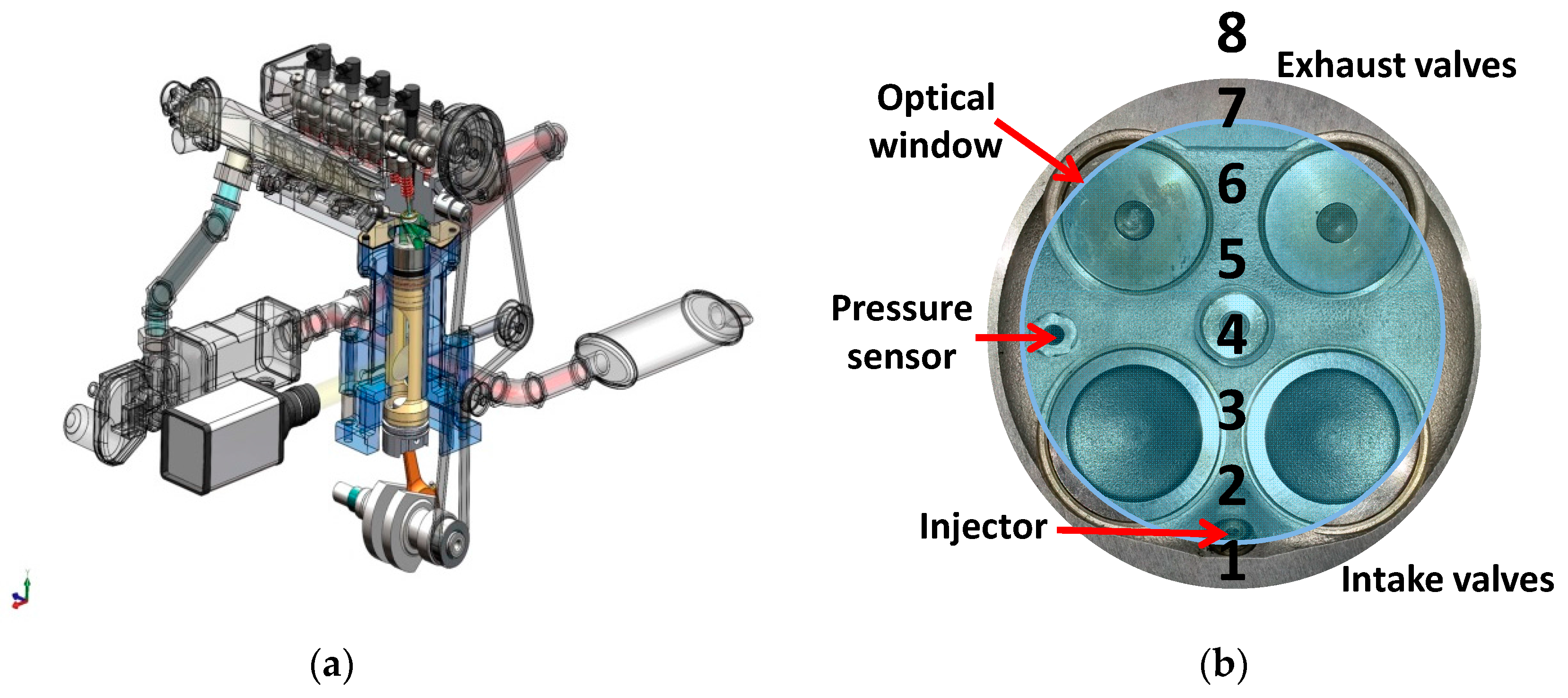
The measurements were performed on an optically accessible single cylinder DISI engine. It was equipped with the four-valve cylinder head of a commercial SI power unit (Figure 1), centrally located semi-surface discharge spark plug, and wall-guided injection. The fuel system featured a commercial six-hole solenoid injector installed in the lateral side of the cylinder head. Further details on the engine are reported in

Table 1. Engine specifications.

Parameter	Description
Displacement	399 cm3
Stroke	81.3 mm
Bore	79.0 mm
Connecting Rod	143 mm
Compression Ratio	10:1
Number of Valves	4
Intake Valves Opening (IVO)	363 CAD BTDC
Intake Valves Closure (IVC)	144 CAD BTDC
Exhaust Valves Opening (EVO)	153 CAD ATDC
Exhaust Valves Closure (EVC)	360 CAD ATDC
Ignition System	central spark plug

.

A conventional Bowditch design was used for optical accessibility, with an optical crown (18 mm thick fused-silica window, which ensured a field of view 63 mm in diameter), which was screwed onto the piston. Therefore, the combustion chamber was visible through a UV-enhanced 45-degree mirror, mounted within the hollow piston. Slotted graphite piston rings were used to provide oil-less lubrication with uninterrupted bronze–Teflon rings used for sealing.

Engine speed was fixed at 1000 rpm in order to study lean burn combustion in low turbulence conditions. The load was fixed in wide open throttle (WOT) mode and the start of injection was also fixed during the intake stroke, at 300 crank angle degrees (CAD) before top dead center (BTDC) to create a homogeneous mixture inside the combustion chamber. Coolant and lubricant temperatures were maintained at 330–335 K using a thermal conditioning unit; intake air temperature was around 300 K and ambient pressure was approximately 1 atm. All measurements were performed at minimum spark timing that ensured maximum brake torque (MBT) (

Table 2. Operating points.

Lambda	Rpm	SA (CAD bTDC)	SOI (CAD bTDC)	DOI (CAD)	Load
1.0	1000	10	300	21.5	WOT
1.3		15		16.5
1.4		20		15.5
1.5		25		14.4
1.6		30		13.5

). The air–fuel ratio was set at stoichiometric conditions, and was then increased until the combustion process became unstable (COV IMEP > 6%). Table 2 shows the increase of spark timing in five CAD steps, with the lambda values augmented; a relatively coarse crank angle (CA) step was chosen, given the flat behavior of the IMEP close to the MBT crank angle.

In-cylinder pressure was acquired with an accuracy of ±1%, and averaged over 200 consecutive engine cycles; the optical measurements were carried out for 25 cycles of each set of 200 cycles. The relative air–fuel ratio was measured using a wide band exhaust gas oxygen sensor, with an accuracy of ±1%. Injection pressure was maintained at 100 bar for all conditions.

Pollutant species concentrations (CO, CO₂, HC and NO_x) were measured in the undiluted exhaust gas stream using an AVL Digas 4000 analyzer (AVL, Graz, Austria), with a resolution of 0.01% (CO), 0.1% (CO₂) and 1 ppm for the other two chemical species, all within 3% accuracy; the measurement principle was an electrochemical sensor for NO_x and non-dispersive infrared (NDIR) analyzer (AVL, Graz, Austria) for the other components. Lastly, smoke opacity was measured by an opacimeter (AVL Opacimeter 439, AVL, Graz, Austria).

2.1. Thermodynamic Analysis

Heat release analysis was performed with a simplified approach of the first law of thermodynamics, using Equation (1):

$$dQ=\frac{\mathsf{\gamma }}{\mathsf{\gamma }-1}·p·dV+\frac{1}{\mathsf{\gamma }-1}·V·dp,$$

(1)

where Q is the net heat released measured in J, p pressure in Pa, V is the cylinder volume in m³, and the ratio of specific heats γ was set to 1.35. Mass fraction burned (MFB) was calculated based on the integral heat release [20,25] via Equation (2):

$$MF{B}_k=\frac{Q_k-Q_{ign}}{Q_{EOC}-Q_{ign}},$$

(2)

where the subscript ‘k’ means the position (CAD) during the combustion process, ‘ign’ denotes the initiation of combustion (ignition), and ‘EOC’ the end of combustion that was considered equal to EVO [25,26]. The combustion process in SI engines can be divided into four main stages [20]: spark and flame initiation, initial flame kernel development, turbulent flame propagation, and flame termination. This process can be quantified with the MFB curve, in which the CA corresponds to 0–10%, MFB is the flame development angle, 10–90% MFB corresponds to the rapid burning angle, and 0–90% MFB is the overall duration of the process. Combustion stability is represented by the cyclic variability derived from pressure data (COV_IMEP).

Lastly, fuel conversion efficiency was calculated using Equation (3):

$${\mathsf{\eta }}_f=\frac{IMEP·V_d}{m_f·LHV},$$

(3)

where ${\mathsf{\eta }}_f$ is the fuel conversion efficiency, IMEP in Pa was calculated based on recorded in-cylinder pressure curves, $V_d$ in m³ corresponds to the displacement volume, and LHV is the lower heating value of gasoline, taken as 42.9 MJ/kg; the mass of fuel injected per cycle $m_f$ was measured in kg, with an accuracy of ±1%.

2.2. Optical Set-Up and Measurement Procedure

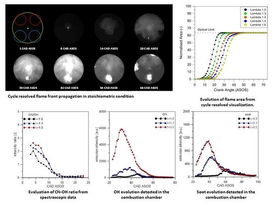
Early flame front propagation was investigated through cycle resolved digital imaging and UV-visible natural emission spectroscopy. Visualization was performed with a high-speed CMOS camera (Optronis CamRecord 5000, 8-bit, 16 μm × 16 μm pixel size) (Optronis, Kehl, Germany) equipped with a 50 mm Nikon objective. The camera worked in full chip configuration (512 × 512 pixel) detecting 5000 frame per second with 200 μs fixed as exposure time. The f-stop of the objective was set at 2.8 to improve the signal to noise ratio without extensive saturation effects. The set-up allowed the acquisition of the images with a dwell time of 200 μs, corresponding to 1.2 CAD at 1000 rpm, and a spatial resolution of 0.188 mm per pixel. The optical trials related to each engine operative condition consisted in the acquisition of 60 frames per cycle after spark timing, during 25 consecutive engine cycles.

Natural emission spectroscopy was applied to follow the evolution of excited chemical species involved in the combustion process from SI until the late combustion phase. UV-visible radiation from the combustion chamber was focused by a 78-mm focal length, f/3.8 UV Nikon objective lens onto the 250 μm micrometric controlled entrance slit of a f/4 spectrometer (Acton SP2150i, Princeton Instruments, Acton, MA, USA) with 150 mm focal length and 300 groove/mm grating (with 300 nm blaze wavelength). The spectrometer was coupled with an intensified charge coupled device (ICCD) camera (Princeton Instruments PI-MAX3 Gen II–UV, Princeton Instruments, Trenton, NJ, USA) provided with a 1024 × 1024-pixel sensor, 16 bit–32 MHz readout, with 45 lp/mm resolution and 0.02 lm/cm² equivalent background illumination. The central wavelength was fixed at 350 nm in order to obtain information in the spectral range of 250–470 nm.

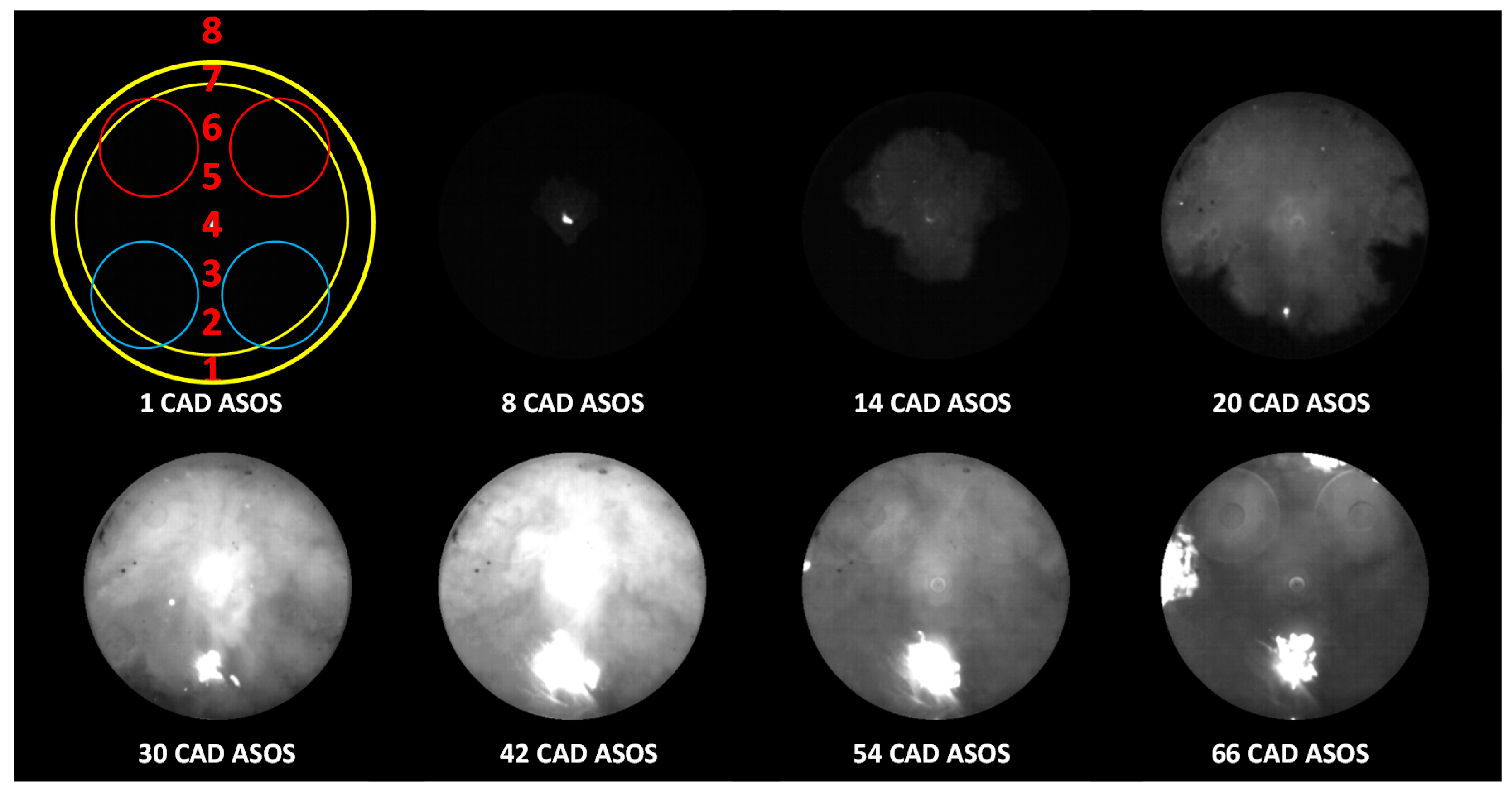
Spectroscopic investigations were carried out in the central region of the combustion chamber. ICCD acquired 1024 spectra that appeared as rows and covered ≈90 mm along the vertical direction. In order to improve the signal-noise ratio, the spectra were binned (128 rows were merged) in eight locations; these were rectangular (≈1.5 × 11.3 mm), as shown in Figure 1. Location 4 corresponded to the spark plug region placed in the center of the combustion chamber, while Locations 2 and 6 corresponded to the intake and exhaust valves region, respectively. Location 8 was intentionally far from the optical limit and it was used as background reference. The ICCD camera operated in sequential mode; 100 acquisitions (eight spectra per frame) were carried out at fixed gate width (40 μs ≅ 0.24 CAD) and increasing delay from spark timing (83.3 μs/cycle ≅ 0.5 CAD/cycle). Synchronization of various control triggers for ignition, injection and cameras was achieved using the optical encoder mounted on the crankshaft as an external clock connected to an AVL Engine Timing Unit (AVL, Graz, Austria).

In order to achieve quantitative information from the optical investigations, image processing of the flame visualization and retrieving procedure of the spectroscopic data were developed.

Image processing allowed the evaluation of macroscopic parameters related to flame morphology by a routine developed in Vision of National Instruments (National Instruments, Austin, TX, USA) [27]. The raw CMOS acquisitions were exported as eight-bit grey-level images. After the extraction of the intensity level, the image processing sequence adjusted the contrast and brightness of the images with respect to the maximum intensity value in order to optimize the signal to noise ratio. Successively, an appropriate circular mask was fixed in order to cut light from reflections at the boundaries of the optical access. Finally, a threshold was applied to obtain binary images. The output of the thresholding operation is a binary image [28,29] whose gray level of 1 (white) will indicate a pixel belonging to the object and a gray level of 0 (black) will indicate the background. A fixed threshold value was chosen for each engine operative condition, since the image sequence maintained an approximately constant difference between the flame intensity and background value during the combustion process. After thresholding, morphological transformations were applied to fill holes and remove small objects that cannot be considered part of the flame and may bias the evaluation of morphological parameters. More details about the procedure are given in [30]. The results of image processing consisted in the flame area A, Waddel disk diameter WDD, circularity FC and flame centroid movement CDM [31]. The flame area A corresponded to the number of pixels included in the foreground of binary images. The Waddel disk diameter was the diameter of a disk with the same area as the binary flame, calculated with Equation (4):

$$WDD=\sqrt{4\times A/\mathsf{\pi }},$$

(4)

where the flame area was obtained by scaling the result in pixels and normalized to the cylinder cross section. The two geometrical parameters provided data useful for a direct comparison with combustion vessel experiments, where similar methods of flame radius growth quantification have been employed for laminar and turbulent flame speed characterizations [32]. The equivalent flame diameter allowed the estimation of the flame speed $S_{t_i}$, calculated using Equation (5):

$$S_{t_i}=\frac{1}{2}\left(\frac{WD{D}_{i-}WD{D}_{i-1}}{\Delta t}\right),$$

(5)

where $WD{D}_i$ is the equivalent flame diameter in correspondence of the frame $i$, $\Delta t$ is the dwell time between two frames. Even though the view from the bottom of the combustion chamber allows only a line-of-sight evaluation and ‘projected burnt area’ would be a more correct phrasing [33], reference will be made to ‘flame area’ and ‘flame speed’ throughout the text. Combined visualization from below and the side in other studies [34] has resulted in a comparable flame front propagation speed during the initial combustion stages; therefore, the methodology used in this study can be considered as representative for the overall propagation speed up to the optical limit. Actual flame front delimitation is a matter of debate, with no clear chemical species accepted as markers that identify reaction zones (even though CH is generally accepted as representative in this sense [35]), and even different types of camera can give close but nonetheless dissimilar flame areas [36]. Nonetheless, the chemiluminescence given by the chemical reactions can be considered as a good evidence of flame front evolution. Regarding its propagation velocity, no unified definition of turbulent flame speed can be found in the literature; in this work, flame speed refers to the measured displacement of the flame front, determined based on the optical data recorded from below the combustion chamber.

The shape of flame fronts was evaluated in terms of Heywood circularity factor FC that corresponds to the ratio between the perimeter P of the image and the circumference of a circle with the same area, according to Equation (6):

$$F{C}_i=\frac{P_i}{\mathsf{\pi }\times WD{D}_i},$$

(6)

where perimeter P_i was obtained by scaling the result measured in pixels. Finally the centroid $CD{M}_i$ was the arithmetical center of the binary flame image of the frame $i$; it was identified by the x and y coordinates with respect to the Cartesian system fixed in the center of the combustion chamber, corresponding to the location of the spark plug.

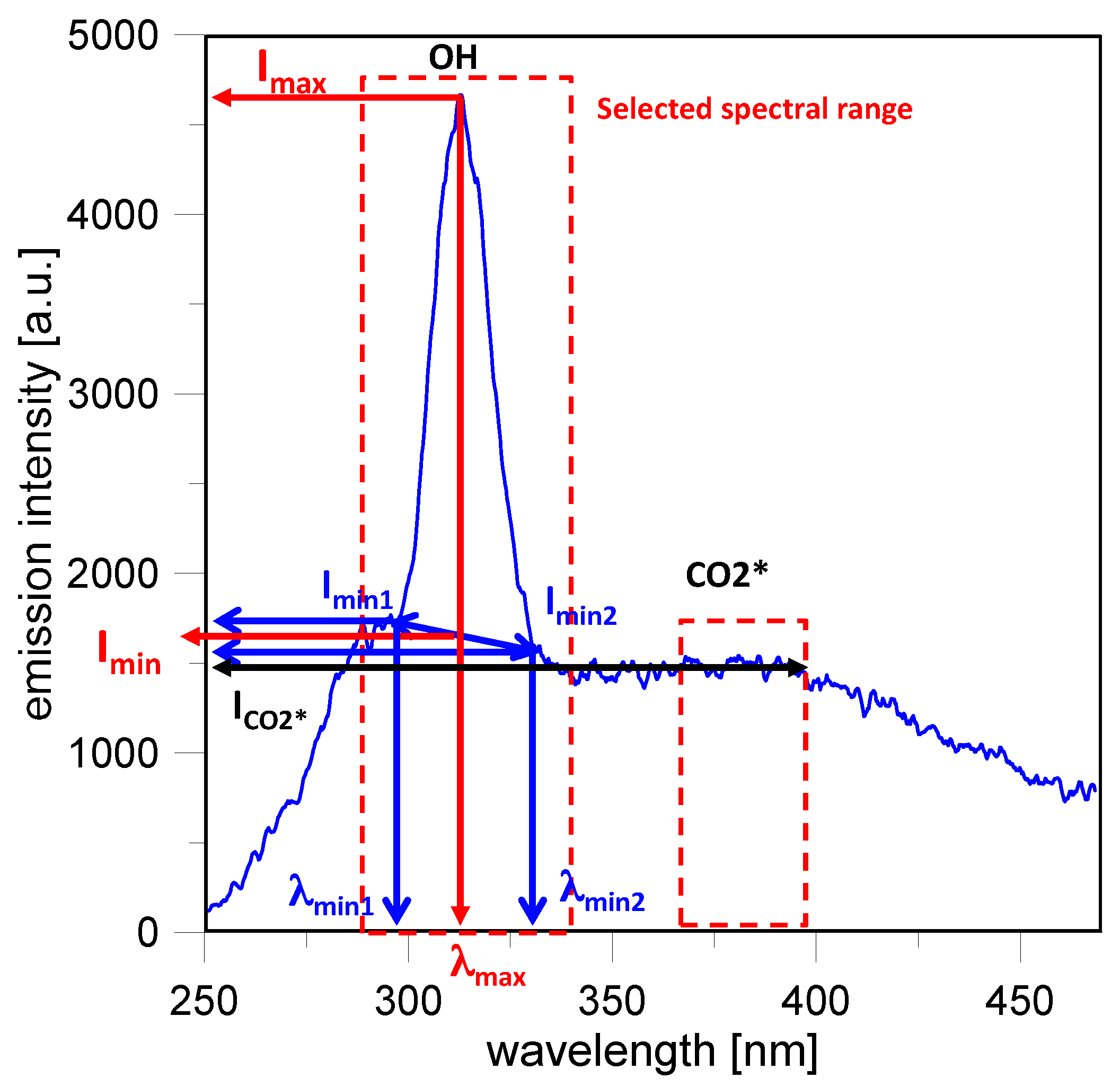
The procedure for retrieving the spectroscopic data was developed in LabView of National Instruments (National Instruments, Austin, TX, USA), following the approach reported in [37]. Specifically, the intensity level of an individual compound (such as OH or CN radicals) was calculated by considering the difference between the highest emission $I_{max}$ in a selected range and the value $I_{min}$ obtained by linearly interpolating the intensities of closest emission minimum, $I\left({\mathsf{\lambda }}_{min1}\right)$ and $I\left({\mathsf{\lambda }}_{min2}\right),$ according to Equations (7)–(9):

$$I=I_{max}-I_{min}$$

(7)

$$I_{max}=I\left({\mathsf{\lambda }}_{max}\right)$$

(8)

$$\frac{{\mathsf{\lambda }}_{max}-{\mathsf{\lambda }}_{min1}}{{\mathsf{\lambda }}_{min2}-{\mathsf{\lambda }}_{min1}}=\frac{I_{min}-I\left({\mathsf{\lambda }}_{min1}\right)}{I\left({\mathsf{\lambda }}_{min2}\right)-I\left({\mathsf{\lambda }}_{min1}\right)}$$

(9)

where local minimum and maximum wavelength values were determined for each component. Figure 2 reports a sketch of the procedure applied for the emission bands related to the OH radical. In the case of broadband emissions, the average intensity in the selected spectral range was considered as representative of the compound’s emission. Specifically for CO₂* the averaged emission from 370 nm to 400 nm was considered; soot emission was evaluated from 460 nm to 470 nm.

3. Results and Discussion

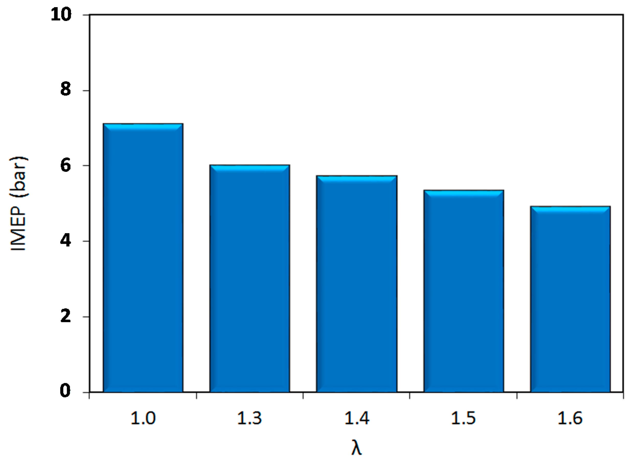
In-cylinder pressure was analyzed as average traces for 200 consecutive acquisitions. As shown in Figure 3, the IMEP decreased as the air–fuel ratio was augmented; this was to be expected, given that the injected fuel quantity was reduced compared to the stoichiometric case. At the limit of lean combustion regime (λ = 1.6) a reduction of around 30% in COV was recorded, with respect to the condition of λ = 1.0. 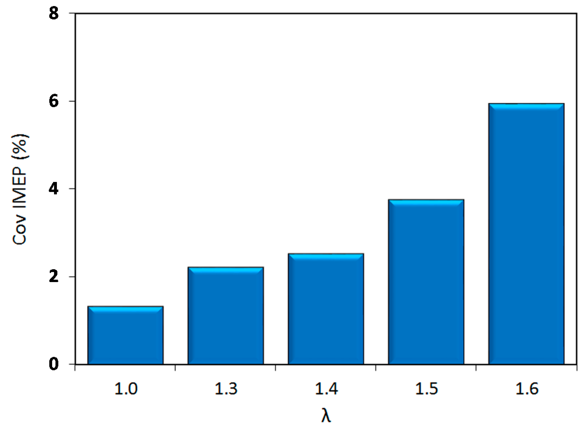Figure 4 depicts the coefficient of variation for the IMEP, as a parameter representative for combustion stability; this graph suggests an increase of cycle by cycle variations with the increase of lambda values. Up to λ = 1.5, stable engine operation was maintained, with COV values below 4%. After this point, instability featured a steep increase with a peak of around 6% for the ‘leanest’ case.

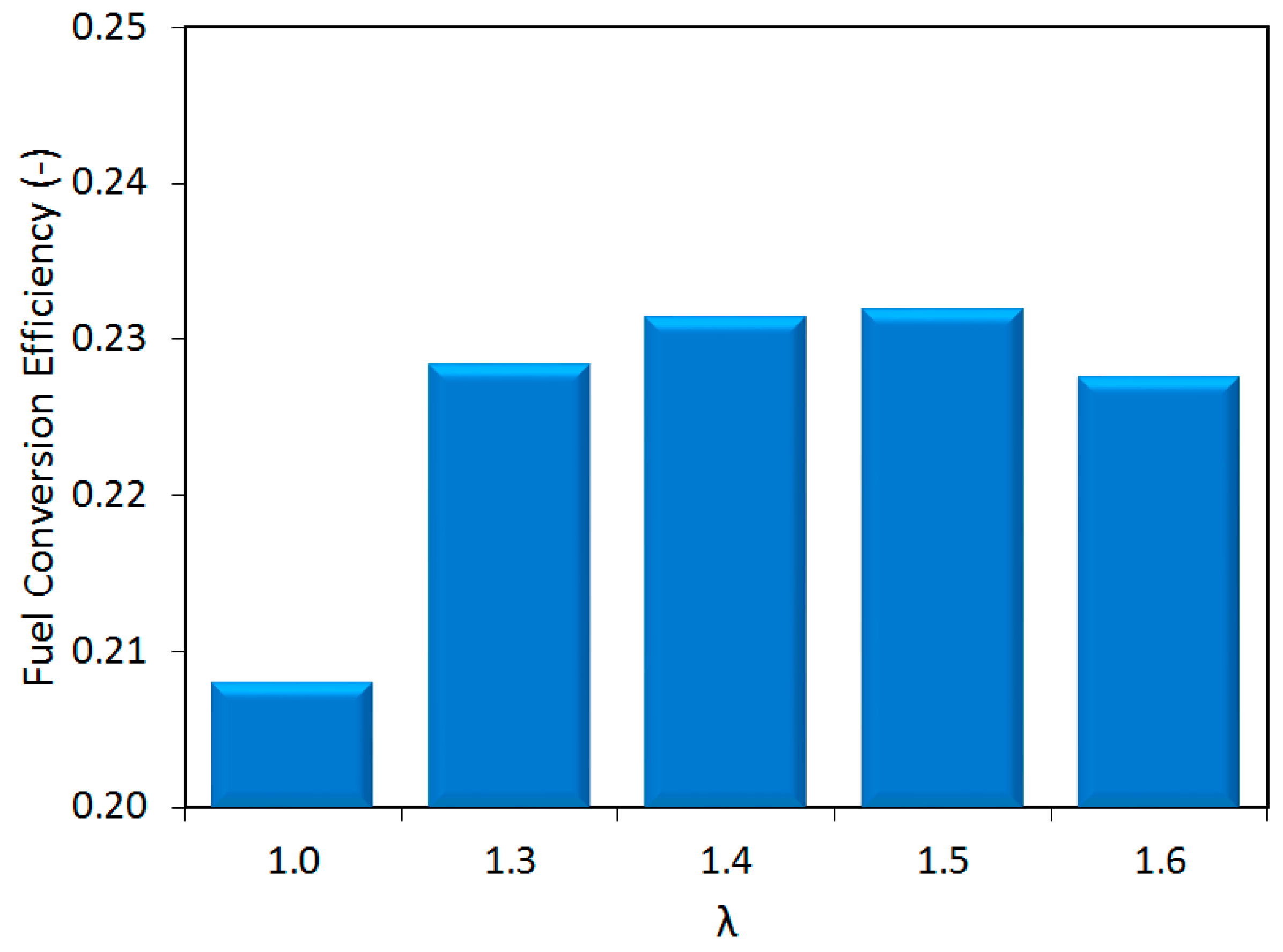
Figure 5 shows the fuel conversion efficiency, calculated as the ratio between work output and chemical energy content of the injected fuel. The stoichiometric case was the ‘least’ efficient, further confirming the need to study the dilute conditions to reduce engine fuel consumption. Moreover, the efficiency increased up to λ = 1.5 and reached its peak slightly over 23%. To put things into perspective, the injected fuel quantity was reduced by over 36% and the IMEP featured a decrease of around 30%, when switching from stoichiometric to λ = 1.6 operation; this explains the increase of around 10% in efficiency when lean air–fuel mixtures were employed.

As the relative air–fuel ratio was varied, two different behaviors become apparent in Figure 4 and Figure 5, in line with well-established trends [20]. Moving along the x-axis (i.e., lambda values), the first regime, which starts at stoichiometric conditions and ends at the location of peak efficiency (λ = 1.5), is characterized by a steadily increasing engine efficiency and low variability. Once over the threshold characterized by peak efficiency, the second regime can be identified, which is characterized by decreasing efficiency and rapidly increasing COV_IMEP. Moreover, in this region, the maximum decrease of the performance (IMEP) was recorded, between two consecutives lambda values, with a reduction of 6% of IMEP for λ = 1.6, with respect to λ = 1.5. 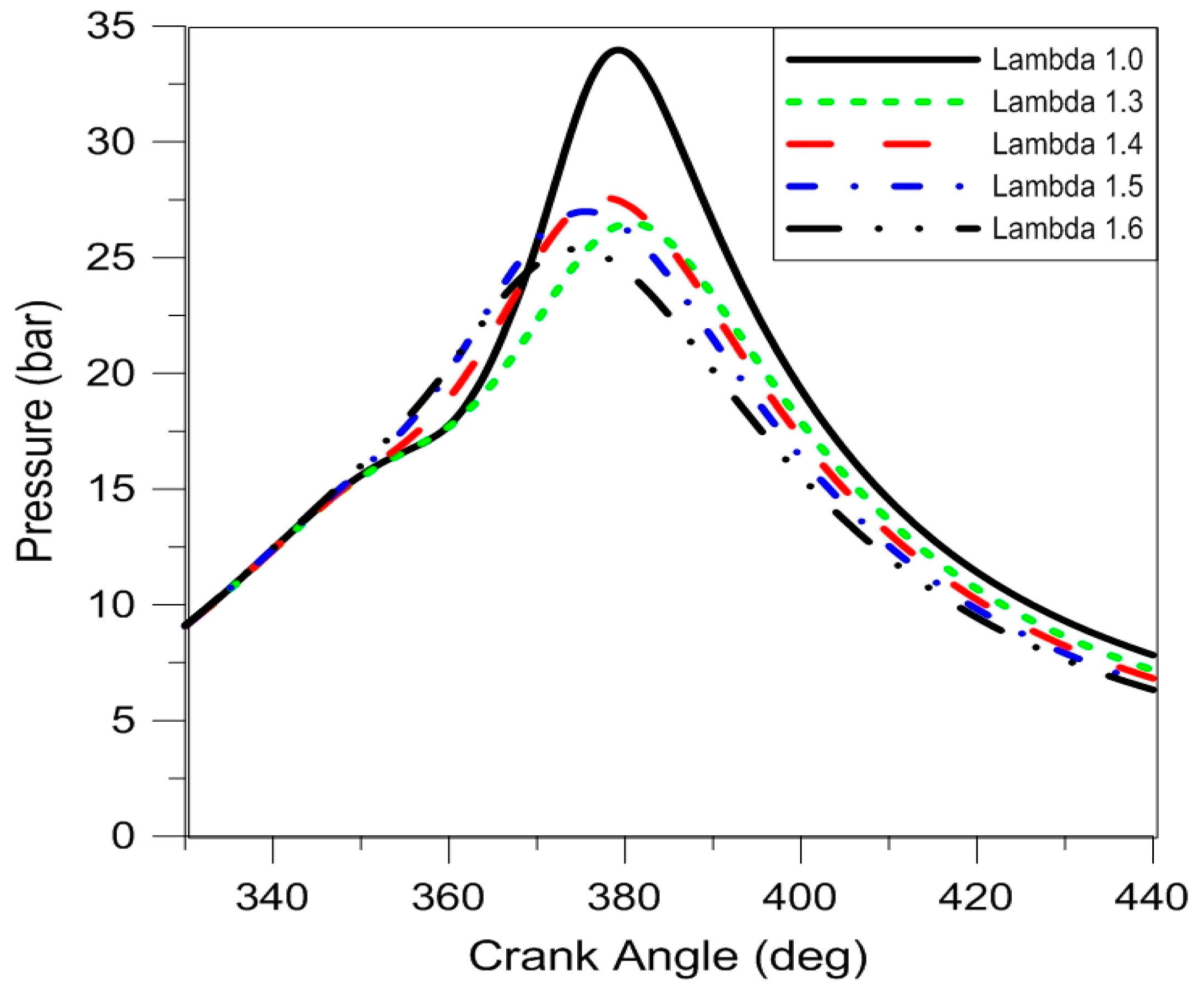Figure 6 reports the average pressure traces of the five air fuel ratios that were tested. It is immediately evident that for stoichiometric operation the highest peak pressure was obtained, as well as overall higher in-cylinder pressure during expansion, in line with the calculated IMEP. The fact that the engine was operated close to the MBT points in each condition is evidenced by the location of peak pressure, within the same range for all air–fuel ratios. As lambda values increase, the main parameter that suffered important changes is the flame development angle (i.e., the initial part of combustion), reflected in more advanced ignition (e.g., start of spark (SOS) needed to be advanced by 20 CAD when switching from stoichiometric to λ = 1.6).

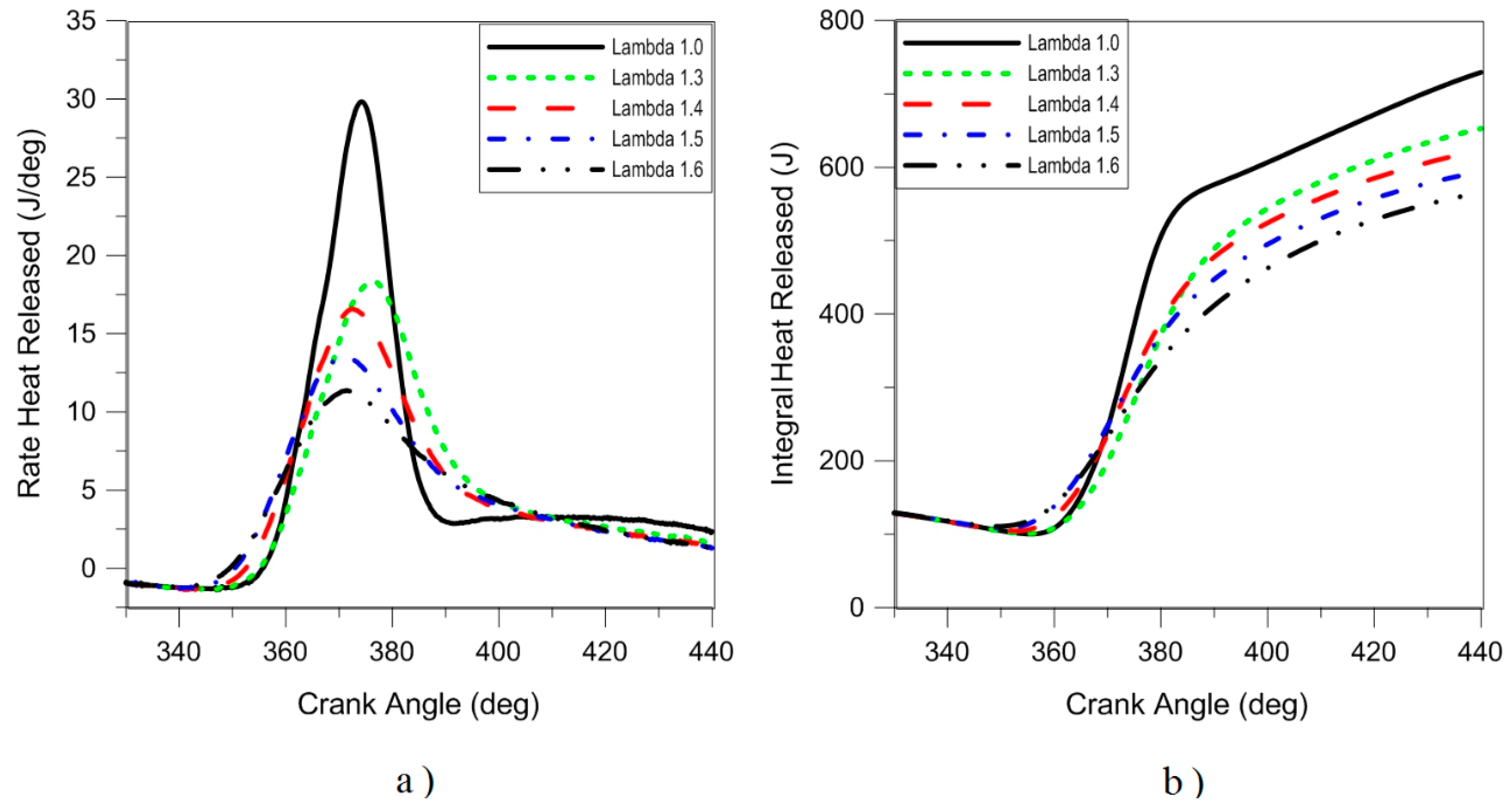
A more detailed analysis of the averaged pressure traces was performed using the heat release approach described in the previous section. Figure 7 depicts the rate of heat release in the combustion process for the stoichiometric and lean burn conditions. As expected, the ‘fastest’ heat release was obtained with λ = 1, while for lean operation ‘smoother’ traces were recorded; this is directly correlated to lower laminar flame speed, resulting in ‘slower’ entrainment and oxidation of the fresh charge. The effect is most evident in the initial stages of combustion, given that flame kernel development is influenced to a large degree by the air–fuel ratio. On the other hand, turbulent flame speed was closer for all cases, which is explained by the effect of turbulence on flame propagation (e.g., S_t = S_L + C_d · r_f/l_M · u′, with S_t as turbulent flame speed, S_L laminar flame speed, C_d dimensionless constant, r_f flame radius, l_M turbulence microscale and u′ turbulence intensity [38]). A common characteristic for all lean cases is more significant rates of heat release during the late stages of combustion, which is well correlated to lower oxidation rates behind the flame front [36].

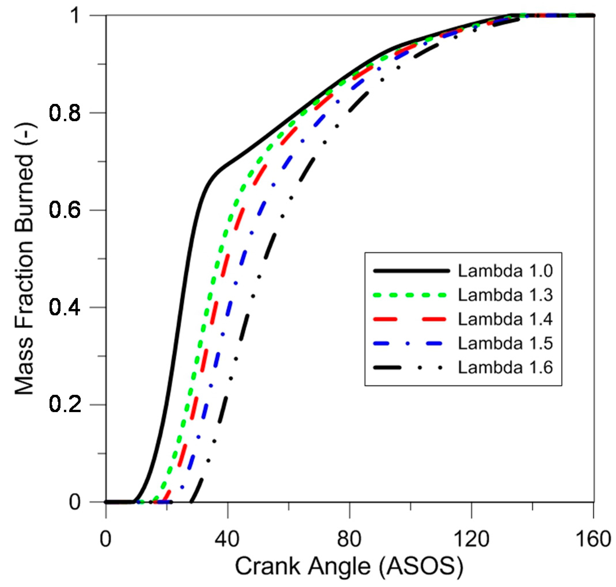
The MFB traces shown in Figure 8 emphasize the fact that each operating point was close to the MTB ignition setting; this effect is more evident compared to the pressure curves (Figure 6), given that the reference point was taken as the SOS. All cases featured quite close evolutions during the final phase of combustion, as this part of the process was controlled by the mass transfer from the top-land region to the cylinder.

Table 3. Burn duration.

Lambda	CA 0–10% MFB	CA 50% MFB
1.0	16.4	377.2
1.3	22.8	382.0
1.4	25.4	379.8
1.5	29.0	380.0
1.6	34.4	382.4

shows several interesting parameters calculated based on the traces shown in Figure 8, which suggest an increase in the duration of the early stage of flame development, as the air–fuel ratio was augmented. Moreover, the maximum increment was registered when passing from lambda 1.5 to 1.6, with a difference of 5.4 CAD. This parameter could be linked with the increment in combustion instability and decrease of the fuel conversion efficiency for the same lambda variation.

Similar values of 50% MFB angle were registered because of the advanced spark timing used in lean burn conditions; this was to be expected, given that ignition was set for operation close to the point of MBT.

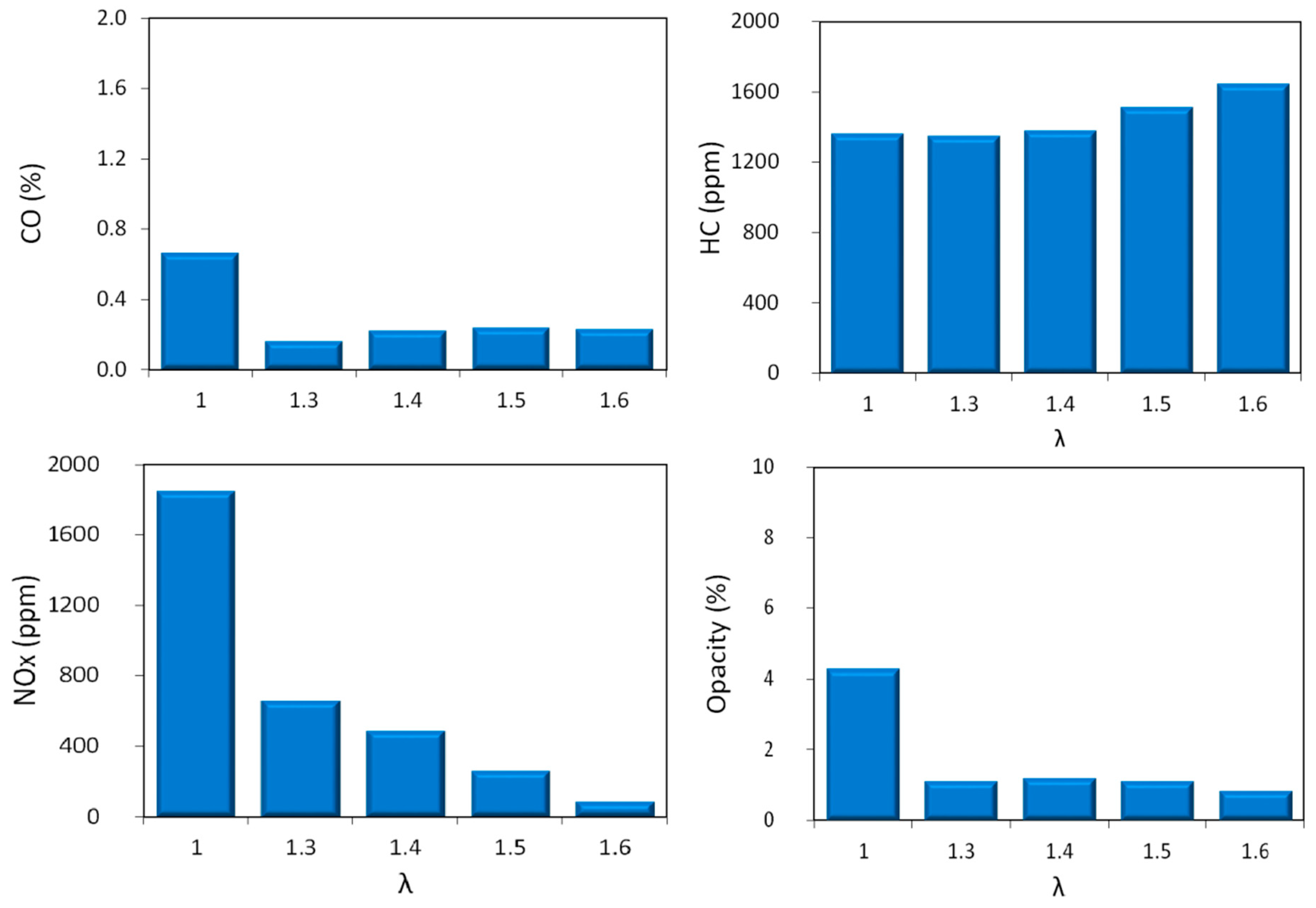
The analysis of exhaust gas measurements gave more information on the chemistry of combustion for the investigated conditions (Figure 9). Carbon monoxide (CO) concentrations were low, with only one case above 0.5% in the stoichiometric condition; this was to be expected, given the increased availability of oxygen in lean conditions. Unburned hydrocarbon (HC) emissions featured shown a flat trend, with a slight increase for diluted conditions. Given that no misfires were detected, this result can be related to more prominent phenomena of quenching near the cylinder wall [20], as the lean flammability was approached. Nonetheless, this mechanism can be considered to have a relatively reduced influence on overall efficiency; to put things into perspective, a concentration of 100 ppm of n-hexane in burned gas (the basis for HC as n-hexane equivalent measurements performed in this study) is equivalent to around 0.5% of the fuel content of stoichiometric air–fuel mixtures. The evolution of nitrogen oxides can be related to the thermal effect [20,39,40] with the highest value for the stoichiometric combustion process. With lean mixtures, the two competing effects (i.e., higher concentration of oxygen and lower burned gas temperature) featured different weights, with temperature having the more prominent influence. For the ‘leanest’ case, a reduction of over 95% in NO_x concentration was recorded. This value was comparable to the efficiency of three way catalytic converters as indicated in [20]. This further emphasizes the potential of lean operation as an option for increasing efficiency and reducing emissions, given that catalytic converters efficiency for reducing CO and HC is high even in lean conditions. When looking at the opacity data, further confirmation of the benefits of lean operation can be identified, with a significant reduction when passing from stoichiometric to λ > 1 region, thus suggesting low particle emissions for the alternative control strategy.

Even if the in-cylinder pressure measurements, coupled with exhaust gas analysis, allow a comprehensive analysis of the combustion characteristics and pollutant formation, they have a global character and do not furnish detailed results of the local distribution of the burned mass. In this sense, cycle resolved visualization represents a powerful tool for quantitative analysis of flame front propagation. 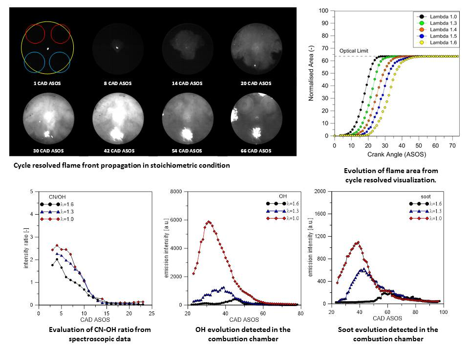Figure 10 shows a selection of images detected in the stoichiometric condition from the first evidence of the spark until the late combustion phase. The spark plug design (i.e., semi-surface discharge) allowed us to detect the flame inception right from the glow phase that can be easily identified by the luminous bright spot in the center of the combustion chamber.

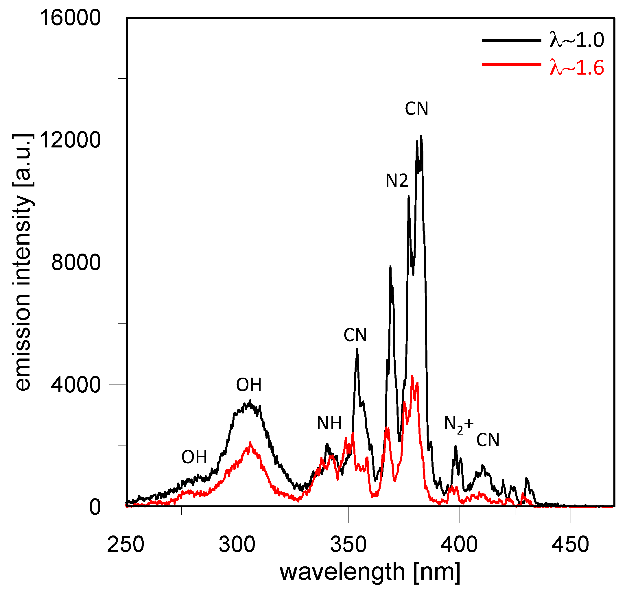
The glow phase featured radiative emissions of CN and OH radicals [41,42,43,44]. As shown in Figure 11, only the highest emission band of the CN violet system B² Σ⁺ → Χ² Σ⁺ at 388 nm were resolved for both cases. The weaker lines at 421 nm and 358 nm were well distinguished only in the stoichiometric case. Similarly, the 309 nm band characteristic of the Α² Σ⁺ → Χ² Π transition for OH radicals was identifiable in all the spectra, while the weaker band at 283 nm was resolved only in the lean burn limit. Other OH lines (such as the band at 314 nm) were too weak to be detected in all the cases. Moreover, the emission due to the N₂ transition C³ Π_u → Β³ Π_g [42,45,46] resulted sufficiently intense to interfere with the CN (0, 0) band. An emission band around 336 nm due to the NH Α² Σ⁺ → Χ² Π electronic transition was also observed, but the intensity resulted too low for the retrieving procedure.

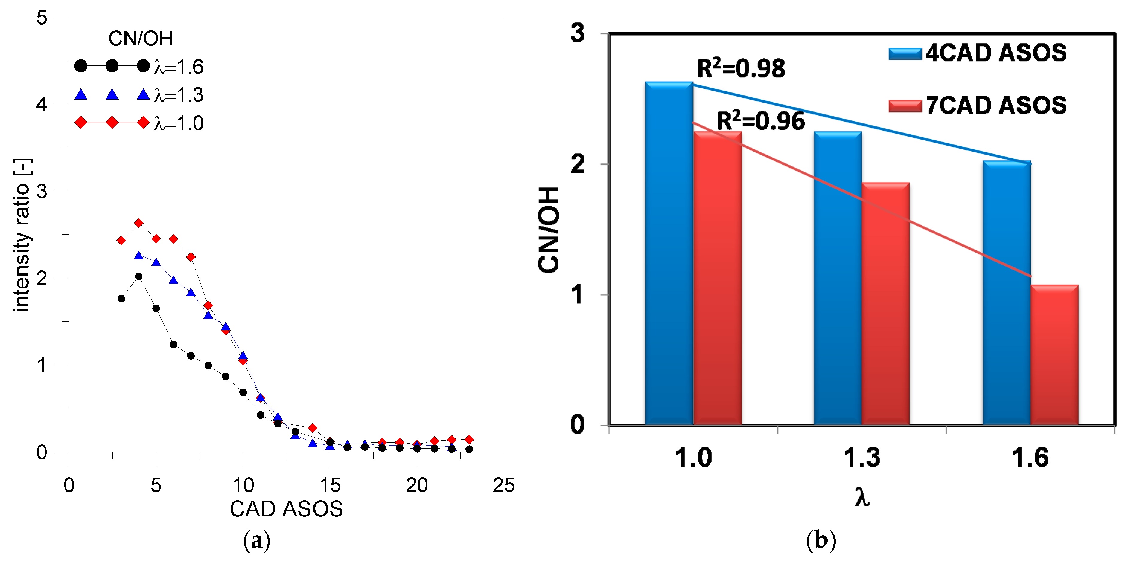
CN emissions at 388 nm were observed until around 15 CAD ASOS, when the end of the glow phase occurred; this result is in agreement with the images of Figure 10 that showed evidence of the spark for about 15–20 CAD after ignition was initiated. Starting from the methodology developed by other authors [47,48,49] and using the retrieving procedure of spectroscopic data, the air–fuel ratio was correlated with background-corrected emission intensity ratio of CN (388 nm)/OH (309 nm) reported in Figure 12a. The averaged values at 4 and 7 CAD ASOS are showed in Figure 12b; the related uncertain was estimated <5%. Results demonstrated a good linear relationship between lambda values and CN/OH ratios. In agreement with the literature [49,50], the change in the pressure near the spark plug determined a change in the linear tendency.

As observed in previous works [25,39,40], flame kernel emission could be well distinguished at around 10 CADs after spark timing due to the luminosity of plasma induced between the spark plug’s electrodes. After this time, the flame front propagated from the center of the combustion towards the cylinder walls. As evidenced in Figure 10, around 15–20 CAD ASOS, a slight asymmetry and significant displacement of the flame were observed towards the exhaust valves. 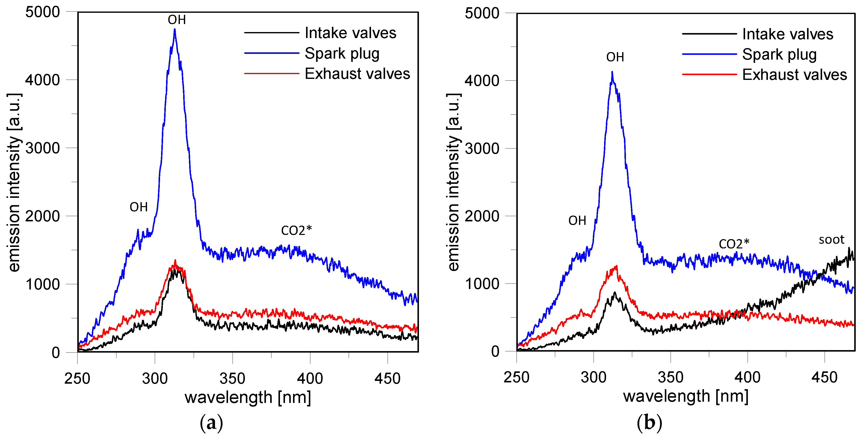The effect can be appreciated also in terms of spectroscopic results, as shown in Figure 13a. Specifically, at 15 CAD ASOS, no evidence of flames could be revealed in the region of the intake valves (Loc. 2); radiative emissions were detected only in the center of the combustion chamber (Loc. 4) and in the region close to the exhaust valves (Loc. 6).

Moreover, no more evidence of CN emission was observed near the spark plug and the spectrum featured high intensity for the OH band at 309 nm. A weak band at 431 nm due to the Α²Δ → Χ²Π CH transition [44] was distinguished. As observed in previous works [37,51], during kernel growth the emission spectra presented a continuum background due to the overlapped emissions of HCO and H₂CO [52,53]. The formyl radical spectrum featured a Vaidya band system that extended from 280 nm to 410 nm, with higher heads in the range of 310–340 nm [54]. Excited formaldehyde emission consisted of diffuse bands between 300 nm and 500 nm (Emeléus system) [55]. The balance between the two species depended on different effects, including local fuel concentration and pressure, which influenced the efficiency of radiative reactions of formaldehyde:

$$\mathrm{HCOH}+\mathrm{h}\mathsf{\nu }\to \mathrm{H}+\mathrm{HCO},\mathrm{HCOH}+\mathrm{h}\mathsf{\nu }\to {\mathrm{H}}_2+\mathrm{HCO}.$$

Formyl radicals successively interacted with oxygen compounds to form CO₂ and H₂O [54].

Spectroscopic investigations demonstrated that the flame front reached the intake valves region (Loc. 2) around 18 CAD ASOS. As shown in Figure 13b, the corresponding spectrum maintained the features previously observed. At the same time, the burned mass at the center of the combustion chamber was characterized by a high-intensity OH band superimposed on a broadband due to excited CO₂ molecules [56,57]. The emissions were extended from approximately 300 nm to 500 nm, with a peak around 400 nm and were most likely induced by the radiative reactions:

$$CO\left({}^1\Sigma \right)+O\left({}^3\Pi \right)\to C{O}_2\left({}^3\mathrm{B}_2\right)$$

$$C{O}_2\left({}^3\mathrm{B}_2\right)\to C{O}_2\left({}^1\mathrm{B}_2\right)$$

$$C{O}_2\left({}^1\mathrm{B}_2\right)\to C{O}_2\left({}^1\Sigma _g^{+}\right)+h\nu .$$

Flame displacement was partially due to fluid motion, basically induced by tumble, and to the different thermal regime between the intake and exhaust side of the combustion chamber. On the other hand, the evidence of high-intensity flames in the intake valve region, near the injector, confirmed the presence of fuel deposits that burned when they interacted with the spark ignited flame front (Figure 10). In agreement with other studies, the deposits determined fuel-rich zones that slowed down the flame propagation [40]. In order to better investigate the effect, the image processing previously described was performed considering the sequences related to 25 consecutive cycles for all lambda values (from 1.0 to 1.6). 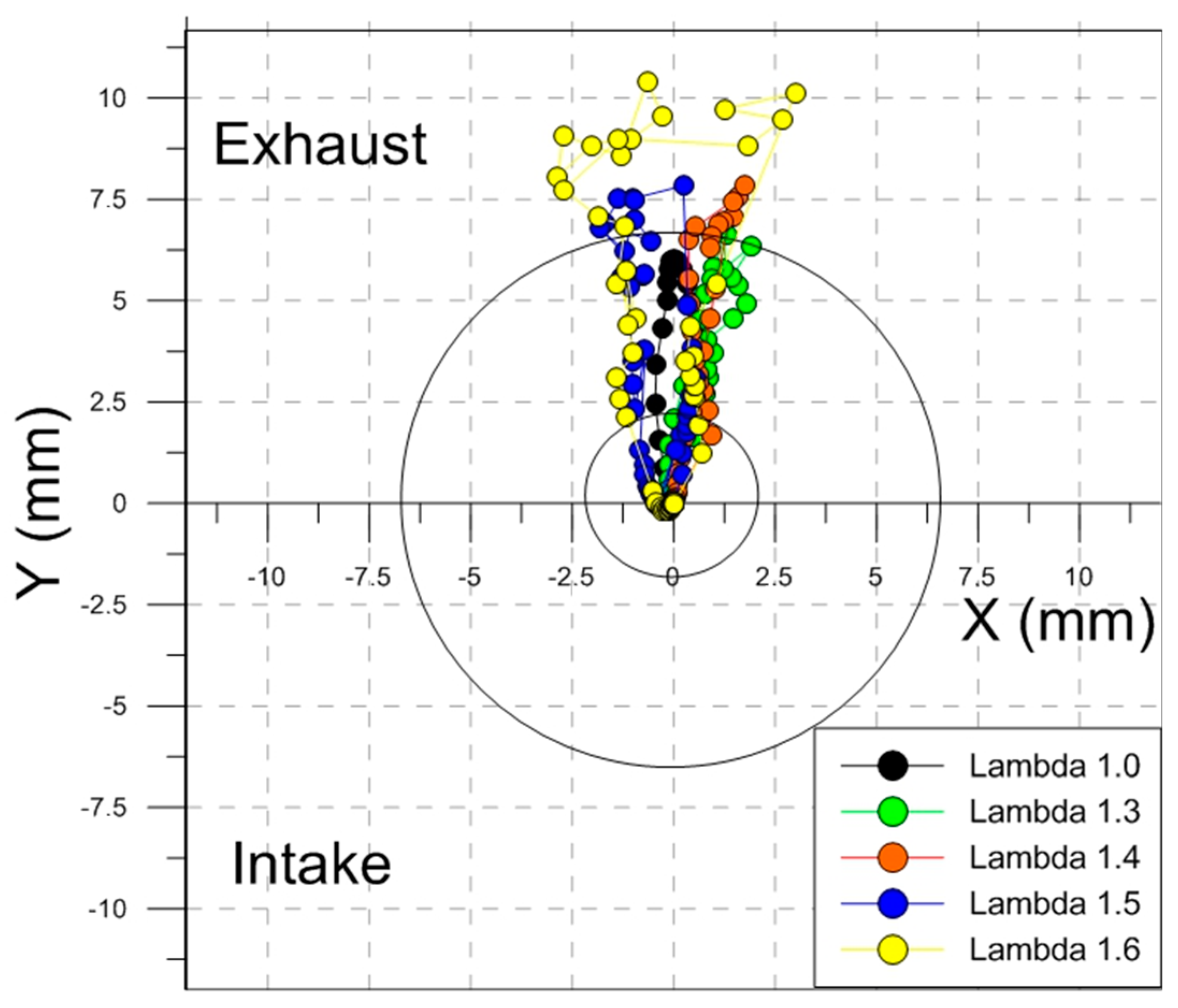Figure 14 shows the evolution of the average luminous centroid with respect to the geometrical center of the combustion chamber, corresponding to the spark plug’s central electrode. X–Y centroid coordinates are biased by a percentage variation <8%. Data are referred to the period of combustion processes between spark timing and the point where flame fronts reached the optical limit. As evidenced in Figure 15a, this duration is strongly related to the air–fuel ratio. Even though the overall propagation was longer for lean mixtures compared to stoichiometric operation, given that the spark timing was advanced for the former cases, the actual crank angle that corresponded to flames reaching the optical limit was within a relatively narrow range (i.e., around 10–15 CAD ATDC). ‘Slower’ lean flames were found to ‘touch’ the optical limit mainly in the exhaust valves region, while stoichiometric combustion featured a more even distribution around the periphery of the cylinder.

The centroid path demonstrated an increasing displacement of the flame as air–fuel mixtures were leaner. This confirmed a more relevant effect of tumble as laminar flame speed was lower; the effect of ignition timing also needs to be considered, given that fluid motion was stronger earlier during the compression stroke, therefore more likely to convect the flame kernel away from the spark plug’s electrodes [34]. A counterclockwise centroid motion was observed for all conditions, due to a slight swirl present during combustion, as identified by the relatively reduced displacement along the x-axis. The path that resulted was slightly wider for leaner conditions, suggesting that flame front progression was biased by the coupling of the in-cylinder flow and the fuel concentration field. 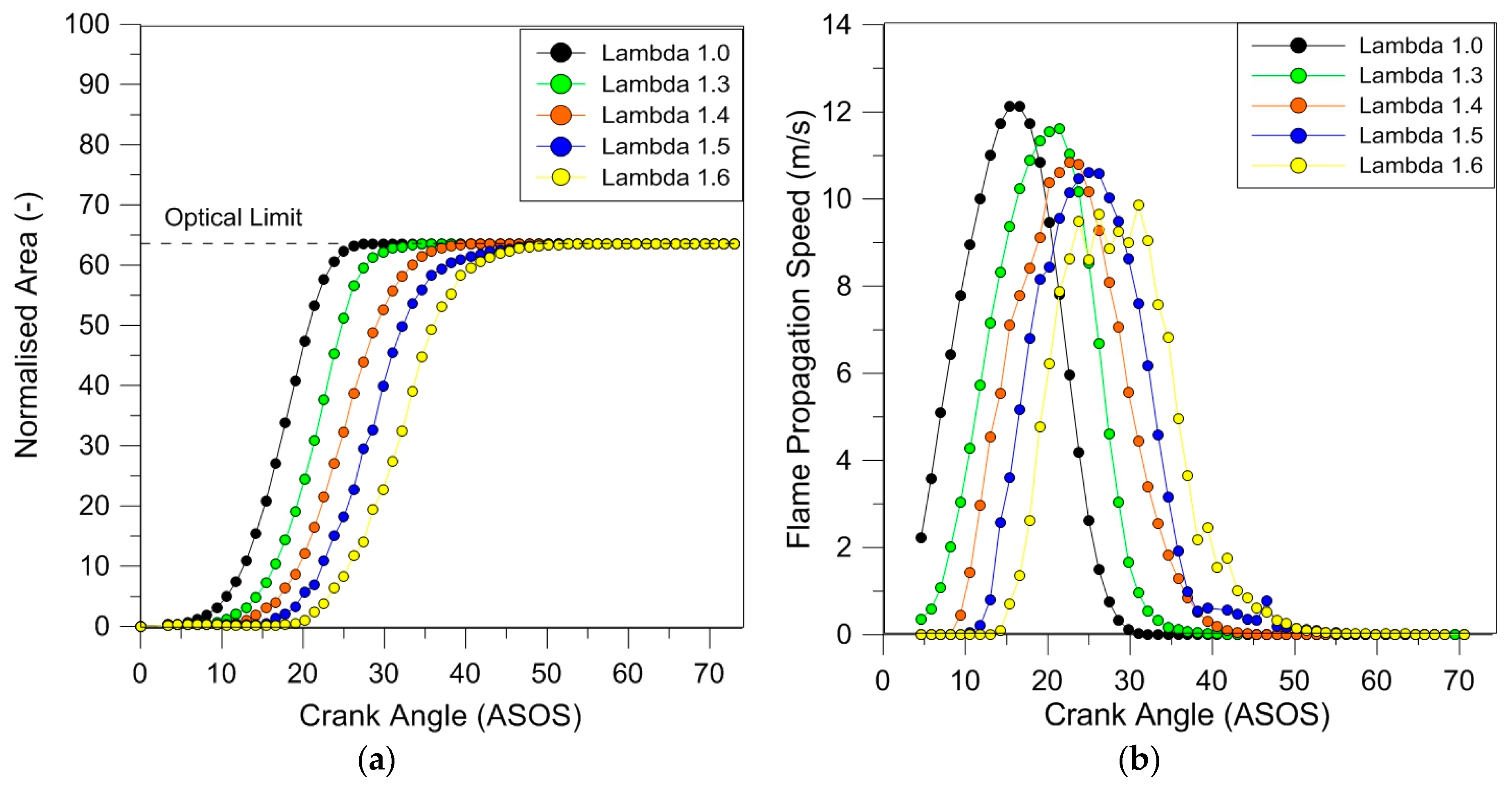Figure 15a,b shows the evolution of flame area and speed. The area was calculated as the average of 25 consecutive sequences and the speed was evaluated by the numerical incremental ratio of the Waddell diameter. The percentage error of flame areas was estimated around 7%. As expected, flame kernel inception (5% of normalized area) was prolonged at increasing lambda values; switching from the stoichiometric ratio to the lean burn limit, this initial combustion phase was longer, 25 CADs for the latter compared 10 CADs for the first case. The effect directly influenced flame front propagation and determined an increase in the time necessary to reach the optical limit at increasing lambda values; this corresponded to a decrease in the laminar flame speed. In terms of average values, the lean burn limit was characterized by a 20% decrease in the highest flame speed (Figure 15b), in line with the previous assertion with regard to turbulent flame speed.

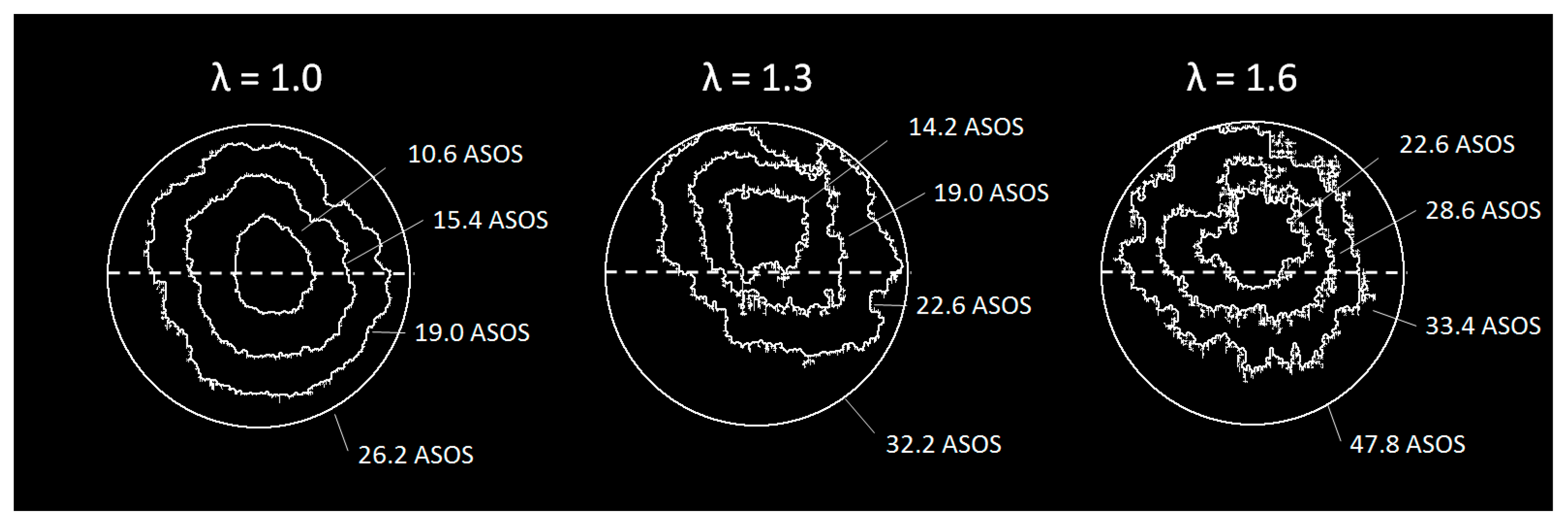
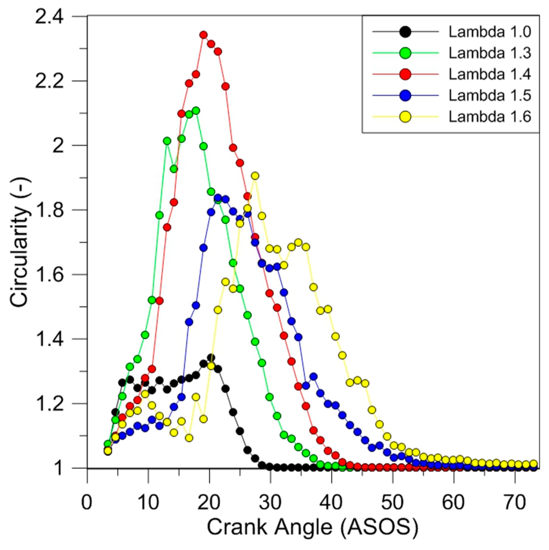
The air–fuel ratio not only influenced the displacement of the flame but also the shape and wrinkling, as it can be appreciated in Figure 16 by the evolution of the flame front contours as they approached the optical limit. To obtain more details on flame morphology, the Heywood Factor was evaluated in each operative condition. Results reported in Figure 17 suggest that for stoichiometric combustion flame propagation spread more uniformly in all directions. On the other hand, in case of diluted operation the simultaneous action of the flow field and fuel distribution determined an increase in the flame distortion. At the lean burn limit, the effect was less evident most likely due to the concomitance of the convection velocity in the swirl plane and tumble motion. This fully fitted the observations reported in [34]. As a consequence of these concurrent phenomena, the highest values of the Heywood factor were found for the case of λ = 1.4.

Regarding the evidence of more wrinkled flames in the diluted cases shown in Figure 16, the results were in good agreement with the analysis performed in [34,58]; these demonstrated that lean flames are more destabilized at fixed turbulence intensity than stoichiometric ones. Vortices in the turbulence field caused flame strain and curvature, ultimately leading to the onset of flame wrinkling and formation of flame pockets [59].

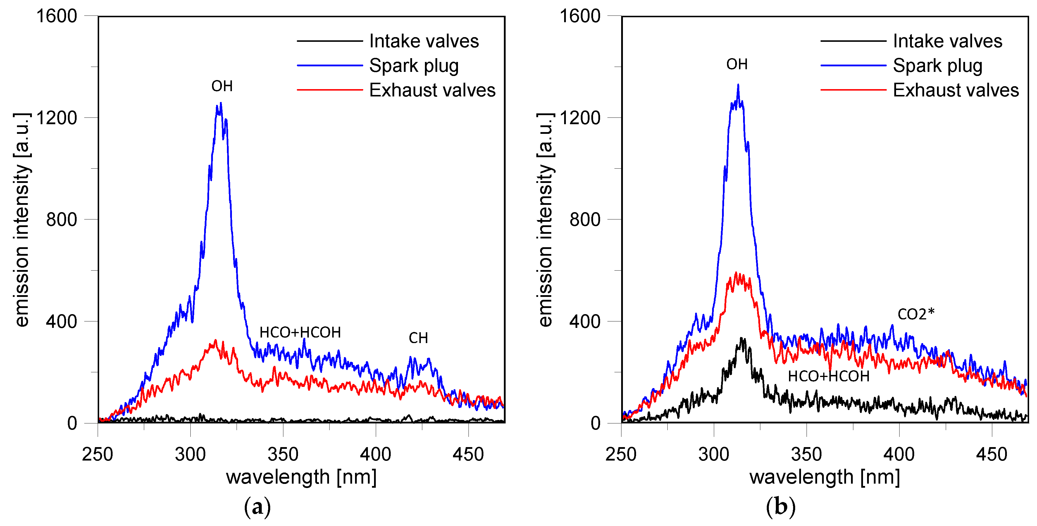
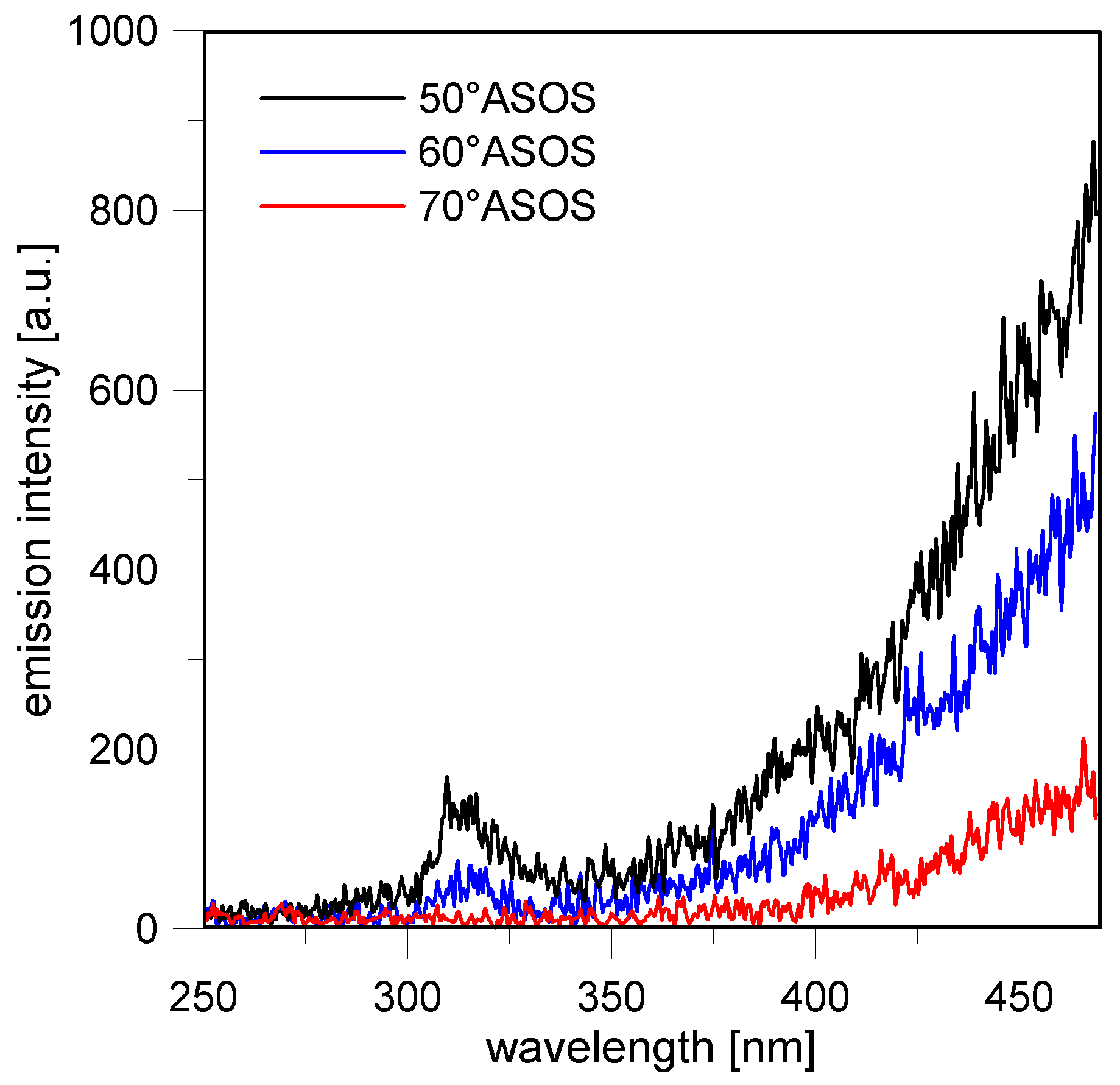
Following the combustion process throughout its progression, from around 20–35 CAD ASOS, the flames reached the optical limit in all investigated conditions. The emission spectra related to the burned gas evolved only in intensity and not in spectral behavior, as can be observed in Figure 18a for the stoichiometric condition. After this time, as shown in Figure 10, strong luminous flames were observed first systematically in the intake valves region and then in random locations near the walls. As observed in previous works [13,39,51,60], these flames were due to the diffusive combustion of stratified fuel in the injector region and on the piston surfaces. In terms of spectroscopic evidence (Figure 18b), these flames featured a continuous signal that increased with a wavelength similar to the blackbody curve described by Planck’s radiation law [61]. The oxidation of fuel deposits induced the formation of carbonaceous structures that formed soot by aggregation. Soot-specific emission was still significant at 70 CAD ASOS in the region near the intake valves for the stoichiometric condition, as shown in Figure 19. These results demonstrate that the fuel deposit flames persisted well after the normal combustion event. Moreover, the spectral evidence of OH confirmed the role of this radical as a fundamental oxidant of soot in turbulent combustion systems, with O₂ being of secondary importance [62].

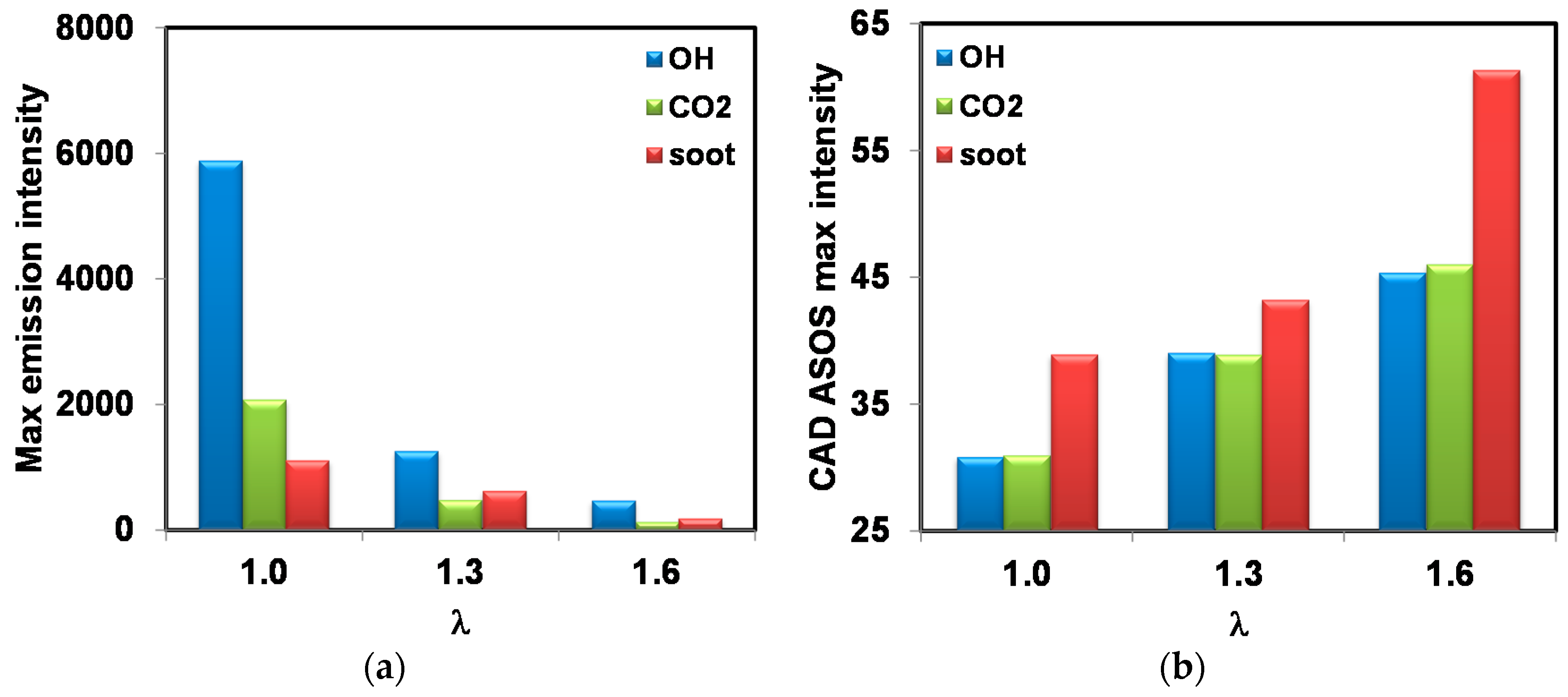
Figure 20 shows the maximum emissions intensity recorded during combustion of OH, CO₂, and soot for three air–fuel ratios. In agreement with results of Ciatti et al. [63], there is an exponential decrease of intensity for all three categories of species, when mixtures were leaner. This is correlated to lower peak pressure values, as well as actual concentrations within the burned/reacting gas. The fact that for λ = 1.6 soot-specific emission was much lower compared to the other two cases emphasizes that particle formation was directly reduced during combustion; on the other hand, with a higher equivalence ratio, the actual measurement at the exhaust was the result of soot formation–oxidation that most likely continued throughout expansion and even during the exhaust stroke. Given the ‘slower’ combustion behavior for lean air–fuel ratios, maximum intensity values were recorded later (at higher CAD values ASOS). For OH and CO₂ these locations were practically the same for each air–fuel ratio, suggesting that these instances were characterized by burned gas with compositions close to chemical equilibrium. Practically, OH radicals can be considered as more representative for intermediate reactions, while CO₂ was specific to completed oxidation, as observed by Irimescu et al [36]. This is very likely given that the instances were around the points of peak pressure, and therefore after flame front propagation was completed. Being the result of diffusive flames induced by fuel deposits, maximum values of soot-specific emissions were recorded later during expansion.

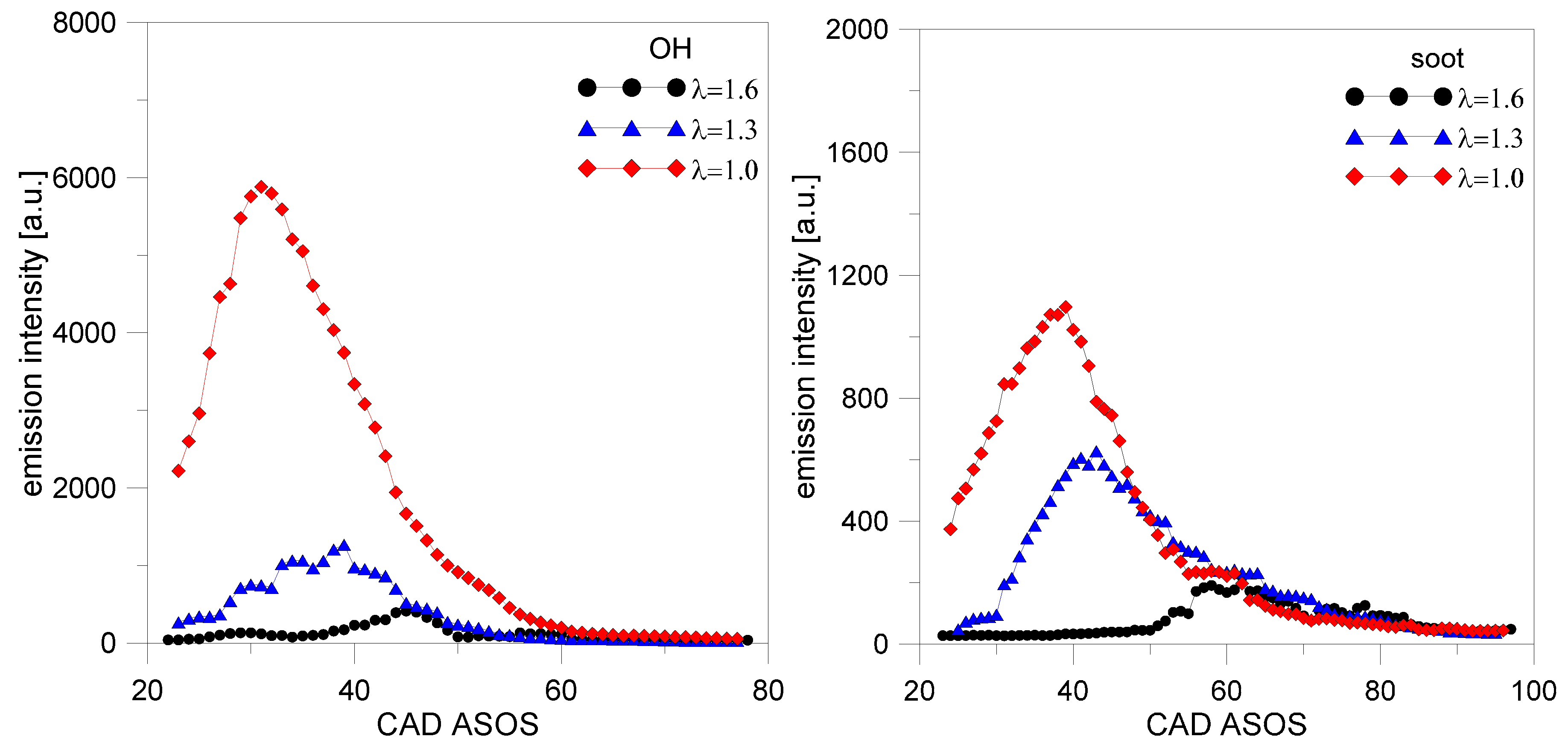
The evolution of emission intensity for OH and soot shown in Figure 21 further emphasizes the effect of gas density on this type of data; the location of peak OH emission is practically the same as that of the in-cylinder pressure traces (see Figure 6 for comparison). As evidenced by the common trend of steep intensification followed by a decrease during expansion, concentrations for both categories of species are related to ongoing oxidation reactions during flame front propagation (in the case of OH) and at the surface of liquid fuel film (for soot).

4. Conclusions

With the goal of providing detailed insight into the specifics of lean combustion in SI engines, the present study employed in-cylinder pressure measurements, determination of exhaust gas concentrations, flame imaging, and spectroscopy. Apart from confirming well-established results related to this engine control mode, the results showed several correlations that were established between physical and chemical phenomena and their evolution during combustion.

As expected, the major conclusion of the thermodynamic analysis was that lean operation ensured an increase of around 10% in fuel conversion efficiency compared to stoichiometric fueling, and acceptable stability, with COV_IMEP slightly over the 5% threshold, even close to the flammability limit of λ = 1.6. Another result was the identification of a prolonged flame kernel phase as the main reason for the requirement of advanced spark timing as air–fuel mixtures were leaner. The analysis of exhaust gas emissions confirmed the potential of lean operation for reducing NO_x emissions, even at levels comparable to the use of three-way catalytic converters. Opacity measurements also showed that this control strategy ensures reduced emission of particles, a pressing issue for GDI engines.

Flame imaging data showed lower overall intensity as the equivalence ratio was lowered, as was to be expected given the lower concentration of reacting species during combustion. Gas density, directly determined by in-cylinder pressure, was the other factor that was identified as a major influence on flame luminosity. Spectroscopy measurements shortly after ignition was initiated showed a very good correlation between the ratio of CN and OH emission intensity and the relative air–fuel ratio; this was determined based on spark characteristics and confirmed the differences in chemical kinetics for each air–fuel ratio setting. Flame area and propagation speed data were in good agreement with the thermodynamic parameters and confirmed the influence of laminar flame speed on overall turbulent flame propagation velocity. Tumble motion was identified as the main factor of influence on flame displacement, and this parameter was found to feature the highest values for λ = 1.6; swirl had only a minor influence overall, but the effect was more prominent for lean operation. An interesting result was that flame circularity showed a decrease as the equivalence ratio was lowered, but over a certain range the trend was reversed, resulting in more circular flames near the flammability limit.

Spectroscopy gave more details of the chemical kinetics of combustion, and showed that burned gas composition was quite similar at different locations within the combustion chamber; this was to be expected, given the injection strategy that comprised of fuel delivery during the intake stroke. A more interesting result was related to the emission intensity recorded for soot precursors that showed particle formation near the injector. The fuel jet impingement sites determined by the injector–piston geometry during injection were coherent with these results and showed a good correlation between the soot-specific intensity recorded during combustion and the measured opacity at the exhaust. The maximum values recorded for the OH, CO₂, and soot ‘spectroscopic signals’, as well as the crank angle of these values, suggested that burned gas composition was close to equilibrium after flame front propagation, and that lean operation ensured much less particle formation due to oxygen availability.

All these findings confirmed the potential of lean fueling for ensuring high efficiency and reduced formation of pollutant species, with acceptable combustion stability. The complete characterization through combined thermodynamic and optical investigations gave more insight into the specifics of combustion process, chemical kinetics, interactions with fluid motion, and the timing of spark-ignited and diffusive flames at the surface of liquid fuel deposits.