Automated Energy Scheduling Algorithms for Residential Demand Response Systems

Abstract

Demand response technology is a key technology for distributing electricity tasks in response to electricity prices in a smart grid system. In the current demand response research, there has been much demand for an automated energy scheduling scheme that uses smart devices for residential customers in the smart grid. In this paper, two automated energy scheduling schemes are proposed for residential smart grid demand response systems: semi-automated scheduling and fully-automated scheduling. If it is possible to set the appliance preference, semi-automated scheduling will be conducted, and if it is impossible, fully-automated scheduling will be operated. The formulated optimization problems consider the electricity bill along with the user convenience. For the fully-automated scheduling, the appliance preference can automatically be found according to appliance type from the electricity consumption statistics. A performance evaluation validates that the proposed scheme shifts operation to avoid peak load, that the electricity bill is significantly reduced, and that user convenience is satisfied.

1. Introduction

In recent years, industry development has occurred rapidly, increasing the demand for electric power. This results in an overload of the electric power supply [1,2]. In particular, the power demand is concentrated at a specific time, thus the frequency of power outages is also increasing. Smart grids are emerging as a new technology to solve such problems by electricity demand control or integration, sustainable mobility, and renewable energy sources; these technologies are essential [3,4]. Among smart grid technologies, demand response (DR) technology is attracting much attention for its ability to intelligently drive the usage of electricity [5,6,7,8]. DR technology and smart equipment help smart grid systems efficiently manage the electricity load in order to optimize electricity resource usage in an intelligent fashion [9]. To adjust the electricity load, DR uses two types of methodologies, which are addressed in the literature: price-based and incentive-based programs [10]. In price-based DR, customers change their electricity usage pattern by rescheduling the appliance or reducing usage during peak periods according to real-time pricing. In incentive-based DR, on the other hand, incentives are provided to customers who use electrical equipment in a manner guided by the grid operator [10]. The focus of this paper is only on a price-based DR program.

Energy scheduling schemes have been the main research topic regarding smart grids. Various energy scheduling techniques for smart grids have been proposed in the literature [11,12,13]. The existing scheduling approaches can be classified by scheduling control strategies as follows. (1) Day-ahead scheduling: scheduling is performed the day before. (2) real-time scheduling: scheduling is performed when an electricity request comes. (3) Multi-scale scheduling: integrating day-ahead and real-time scheduling [14]. This paper focuses on day-ahead scheduling.

The existing energy scheduling approaches usually target at least one of the following scheduling goals: reducing the electricity bill, reducing peak consumption, and improving user convenience.

Research efforts using additional optimization variables such as user convenience [11,15,16] have been recently presented as opposed to using only the electricity bill and peak consumption. These studies argue that users are trying to reduce the electricity bill without sacrificing the user’s convenience. To achieve an acceptable trade-off between minimizing the payment and waiting time for the operation of each household appliance under the peak consumption constraint, Mohsenian-Rad and Leon-Garcia [11] proposed a residential energy scheduling scheme. However, this scheduling scheme does not consider various types of appliances, instead only focusing on appliances that can be reserved. Yi et al. [15] proposed an energy scheduling scheme that uses a stopping method to achieve the minimum electricity bill and waiting time in a smart grid. They make a fake schedule based on the optimal stopping approach at the first stage as if there are no power constraints. Then, the power constraints are taken into account at the second stage. This scheduling scheme, however, does not consider the operation duration of the appliances, and thus cannot meet the user convenience requirement for appliances. Similarly, the above scheduling approaches using user convenience do not consider the various types of possible devices, nor do they consider the appliance deadline. For user convenience, Chen et al. [16] divided the energy scheduling tasks into two types: delay-tolerant and delay-intolerant tasks. In delay-intolerant tasks, activating the device immediately upon its arrival is the only choice. On the other hand, to make use of the fluctuating nature of the electricity price, delay-tolerant tasks can be opportunistically scheduled. In day-ahead scheduling, classification according to the tolerance is not suitable since it cannot shift the load to an earlier time. For day-ahead scheduling, this paper classifies the appliance according to schedulability and interruptability.

Additionally, a smartphone-based energy scheduling methodology considering a large variety of deployment scenarios, due to the increasing demand for smartphones for use as control entities in smart grids, should be developed. In particular, smartphones are an attractive control and monitoring tool for energy scheduling in a smart grid. In addition, smart appliances are evolving into intelligent functions that can be operated through smartphones [17,18,19]. By using smartphones and smart appliances, the customer can easily adjust their energy schedule and monitor their electricity usage. Further, smartphone applications can remotely control smart appliance operation periods. For instance, a number of consumer electronics companies have recently started to provide smart appliance controls through smartphones. Through a simple procedure using a smartphone, customers can easily and remotely register and control their home appliances.

With the development of DR and smart appliances, fully-automated scheduling is possible in residential smart grids. However, previous studies [11,15,16,20] are limited in that they assume that the user sets the preferred operation time for each appliance (the preferred time is referred to as user convenience in this paper). In this paper, a demand response scheme is proposed that automatically estimates a user’s convenience without configuring the convenience for fully-automated energy scheduling. The proposed scheme provides the following contributions:

• A mathematical model is established to minimize the electricity costs and maximize the user convenience, which is computed as a function of the operation time.
• Two automated scheduling schemes are proposed. If the user sets the preferred time sections of the appliances, the proposed scheme can automatically schedule the appliances according to the preferred time section (referred to as semi-automated scheduling). If the user cannot set the preferred time of the appliances, the proposed scheme can search for the preference based on the usage statistics and then automatically schedule the appliances (referred to as fully-automated scheduling).
• Appliances are classified according to operation type. Then, a scheme that can estimate the preference time according to the classification based on the usage statistics pattern is proposed.

The rest of this paper is organized as follows. In Section 2, the system architecture and model are introduced. The fully-automated scheduling algorithm is given and optimization problems are formulated in Section 3. Simulation results are given in Section 4. Finally, this paper is concluded in Section 5.

2. System Architecture and Model

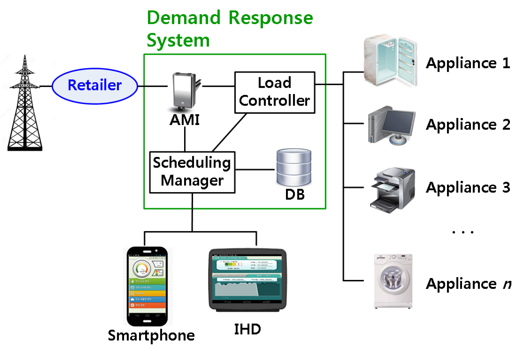
2.1. System Architecture

This section introduces the system architecture. In general, the overall composition of the smart grid system contains the power utility/retailer, advanced metering infrastructure (AMI), load controller, scheduling manager, database, and a number of appliances. In the proposed system architecture, the smart grid system contains additional equipment such as an in-home display (IHD) or smartphone in order to provide convenience to the user. The relationship among these systems is shown in Figure 1.

By using a smartphone or IHD, a user navigates the smart grid system, checking their electronic bill, monitoring their energy consumption, requesting user convenience, and monitoring their scheduling results. To request user convenience, the user sets their preferred begin operation time and end operation time for each appliance. If the scheduling results of the appliance are between the start time and the end time, the scheduling result is said to satisfy the user convenience. If the scheduling results of the appliances are mismatched with the user’s preferred time, the user convenience will decrease in proportion to the time gap.

As shown in Figure 1, the demand response system contains the AMI, load controller, scheduling  manager, and database. The AMI is able to communicate in two ways between a residential smart grid system and the retailer company through a local area network (LAN). Assume that the AMI receives real-time pricing data from the retailer. The real-time pricing data is delivered to the scheduling manager to compute the scheduling strategy. The load controller is a connect point between the demand response system and appliances. When the load controller receives the scheduling results from the scheduling manager, it can then operate each appliance based on the scheduling results. Moreover, the load controller receives the energy consumption information for each appliance. Then, the information will be delivered to the scheduling manager. The database is used to store the appliances’ usage patterns. These usage patterns can be converted into user convenience to calculate the next schedule. For the scheduling strategy, the scheduling manager collects information regarding the user convenience, real-time pricing, and energy consumption. The scheduling manager sends the scheduling result to the load controller to operate the appliances. The user can monitor the scheduling results by using a smartphone or IHD.

In the proposed system architecture, each smart grid element has the following perspectives. The user normally intends to minimize their electricity cost while satisfying user convenience. Therefore, the user consumes electricity by taking into account real-time pricing and user convenience. Power utilities are primarily responsible for providing quality power to users and preventing system blackouts. To prevent blackouts, the utility uses the real-time pricing policy that increases the price when the consumption is concentrated. Therefore, electricity consumption can be dispersed.

In general, the operation of some appliances may not be time shiftable or controllable. For example, motion detectors or smoke detectors may not be time shiftable since they have to be on all of the time. On the other hand, a television may not be controllable because it usually turns on unpredictably. Therefore, the appliances are categorized according to their controllability as follows [20].

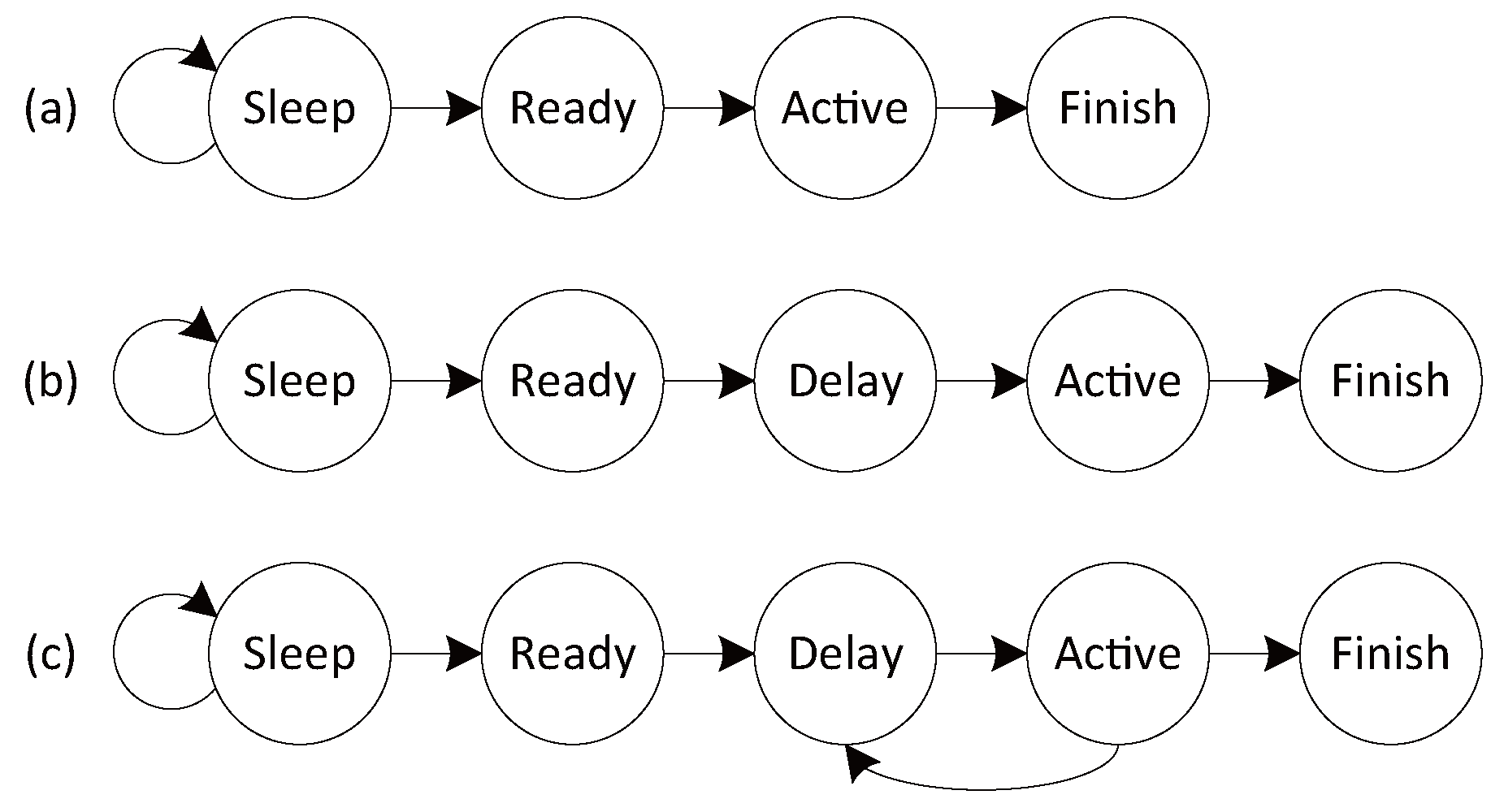
• As mentioned earlier, the operation of some appliances may not be controllable. These appliances are referred to as uncontrollable appliances. Lighting systems, computers, televisions, and hair dryers are examples of uncontrollable appliances. Thus, they cannot be controlled by the load controller. However, they should provide their power consumption and operating information to the load controller since the smart grid system has strict energy consumption scheduling constraints. Figure 2a shows the state diagram of an uncontrollable appliance. When the appliance does not operate, it sleeps. If it receives an operation command from the user, it will then be activated.
• Although the start time could be controlled, there are some appliances that cannot be stopped during operation. These appliances are referred to as non-interruptable appliances. Non-interruptable appliances include dishwashers and washing machines. When a smart grid system calculates the scheduling strategy, the non-interruptable appliances should be scheduled continuously. Figure 2b shows the state diagram of a non-interruptable appliance. When the appliance does not operate, it sleeps. If it receives an operation command from the load controller, it will wait until the scheduled time and then be activated.
• In contrast to non-interruptable appliances, some appliances can be stopped during their operation time. These appliances are referred to as interruptable appliances. Interruptable appliances include house heat ventilation air conditioning (HVAC), water heaters, and plugged hybrid electric vehicles (PHEVs). They can be scheduled at discrete times to avoid the peak load increasing. Figure 2c shows the state diagram of an interruptable appliance. When the appliance does not operate, it sleeps. If it receives an operation command from the load controller, it will wait until the scheduled time and then activate. After being activated, it can stop operation and will then complete the remaining job.

2.2. Demand Response Model

In this section, the energy scheduling optimization problem in a real-time pricing environment is formulated. The objective of the optimization problem is to minimize the electricity bill and maximize the user convenience. In this paper, assume that the real-time pricing information is provided from the power retailer at the beginning of the day (i.e., assume day-ahead pricing).

Assume that timeslot t is divided into equal unit times and denote by $\mathcal{T}$ the set of timeslots.

$$t\in \mathcal{T}\triangleq \{1,\dots ,T\},$$

(1)

where T is the end of the time. In this paper, assume $T=24$.

Let $\mathcal{A}$ denote the set of appliances. For each appliance $a\in \mathcal{A}$, a consumes an amount of electricity $E_a^{on}$ when it operates. Denote by $I_a^t$ a scheduling indicator function of appliance a at t, where $I_a^t$ is 1 if appliance a is scheduled and 0 otherwise. Assume that a requires a certain number of timeslots for operation, denoted by $T_a$. Therefore, Equation (2) is derived.

$$T_a=\sum _{t\in \mathcal{T}}{I}_a^t.$$

(2)

As mentioned in Section 2.1, the appliance type is categorized as shown the Figure 2. Denote by ${\varphi }_a$ the appliance type of appliance a, which is expressed by

$${\varphi }_a=\left\{\begin{array}{cc}0,\hfill & \mathrm{if}\mathrm{appliance}\mathrm{type}\mathrm{of}a\mathrm{is}\mathrm{uncontrollable}\hfill \\ 1,\hfill & \mathrm{if}\mathrm{appliance}\mathrm{type}\mathrm{of}a\mathrm{is}\mathrm{non-interruptible}\hfill \\ 2,\hfill & \mathrm{if}\mathrm{appliance}\mathrm{type}\mathrm{of}a\mathrm{is}\mathrm{interruptible}.\hfill \end{array}\right.$$

(3)

In order to prevent system blackout, the energy consumption at time t has a maximum limitation $BO$, i.e.,

$$\sum _{a_a\in A}{I}_a^t·E_a^{on}\le BO.$$

(4)

As aforementioned, assume that the energy management system receives day-ahead real-time pricing from the power retailer. Figure 3 shows the time-varying price provided by the Illinois Power Company (Springfield, IL, USA) on 15 December 2009.

Denote by $p^t$ the real-time pricing at timeslot t. Therefore, the cost function $B(·)$ can be formulated as Equation (5).

$$B(·)=\sum _{a\in \mathcal{A}}{p}^t·I_a^t·E_a^{on}.$$

(5)

In the proposed scheme, the user convenience is considered to be as important as the electricity cost. Therefore, a user convenience model is used that is determined according to the scheduling timeslot. As mentioned above, assume that each appliance has a preferred operation time. Denote by ${\alpha }_a$ the preferred starting timeslot and ${\beta }_a$ the preferred ending time of appliance a, where ${\alpha }_a<{\beta }_a$ and ${\alpha }_a,{\beta }_a\in \mathcal{T}$. Suppose that for a dish washer (a), the user wants a to work from lunch time (13:00) until dinner time (18:00). In that case, the preferred starting time ${\alpha }_a=13$ and preferred ending time ${\beta }_a=18$ should be set. In addition, ${\beta }_a-{\alpha }_a$ is equal to or greater than $T_a$. For the convenience metric, an operation should be scheduled during the preferred time. If the scheduling is advanced or delayed, however, the user will experience discomfort. Therefore, the user dissatisfaction can be calculated using the number of timeslots that are non-overlapping with the preferred time. Denote by $v_a$ the total number of time slots non-overlapping with the user preferred time, which is obtained by Equation (6).

$$v_a=\sum _{t=1}^{{\alpha }_a-1}{I}_a^t+\sum _{t={\beta }_a+1}^T{I}_a^t.$$

(6)

If dissatisfaction is measured by the number of timeslots that are non-overlapping with the preferred time, the following problem will occur. Figure 4 shows two cases of scheduling results if ${\alpha }_a=1$ and ${\beta }_a=6$. The scheduling result of case (a) is from 7 to 9 and the result of case (b) is from 10 to 12. Although case (a) is scheduled closer to the preferred time than case (b), the dissatisfaction is calculated to be equal (i.e., $v_a$ is 3.) Therefore, the dissatisfaction degree $w_a^t$ is introduced, which is expressed in three cases:

$$w_a^t=\left\{\begin{array}{cc}\hfill {\alpha }_a-t,& t<{\alpha }_a\hfill \\ \hfill 0,& {\alpha }_a\le t<{\beta }_a\hfill \\ \hfill t-{\beta }_a+1,& {\beta }_a\le t.\hfill \end{array}\right.$$

(7)

$w_a^t$ increases the further away it is from the preferred time. The dissatisfaction can be represented as the product of $w_a^t$ and $I_a^t$. (i.e., ${\sum }_{t\in \mathcal{T}}{w}_a^t·I_a^t$.) If this version of dissatisfaction is used, $v_a$ is 6 in case (a) and $v_a$ is 15 in case (b). In this case, however, appliances with longer operating times have a greater dissatisfaction. Figure 5 shows two example cases of appliances that have the same preference time but have different operating times. Although case (c) is not scheduled at all at the preferred time and case (d) is scheduled at some preferred time, both (c) and (d) have the same dissatisfaction of 6. However, the user will likely be more dissatisfied in case (c). For this reason, divide ${\sum }_{t\in \mathcal{T}}{w}_a^t·I_a^t$ by the operating time of the appliance and formulate a dissatisfaction function $D(·)$ as Equation (8) [20].

$$D(·)=\sum _{a\in \mathcal{A}}\sum _{t\in \mathcal{T}}\frac{w_a^t·I_a^t}{T_a},$$

(8)

where $w_a^t$ is calculated by Equation (7).

Considering Equation (8), the dissatisfactions are 2, 5, 2 and 1 for cases (a), (b), (c), and (d), respectively.

Moreover, the appliance type needs to be reconsidered. In particular, uncontrollable appliances and interruptible appliances need extra constraints. Uncontrollable appliances should be scheduled in their preferred time. Therefore, Equation (9) is derived as:

$$\sum _{t={\alpha }_a}^{{\beta }_a}{I}_a^t\ge T_a,\forall {\varphi }_a=0.$$

(9)

On the other hand, non-interruptible appliances cannot stop during operation. (i.e., the sum of the changes of adjacent $I_a^t$ values should be 2 except when $I_a^t$ for the first and last timeslots are set to one.) Therefore, Equation (10) is derived as:

$$\sum _{t=1}^{T-1}{(I_a^t-I_a^{t-1})}^2\le 2-I_a^1-I_a^T,\forall {\varphi }_a=1.$$

(10)

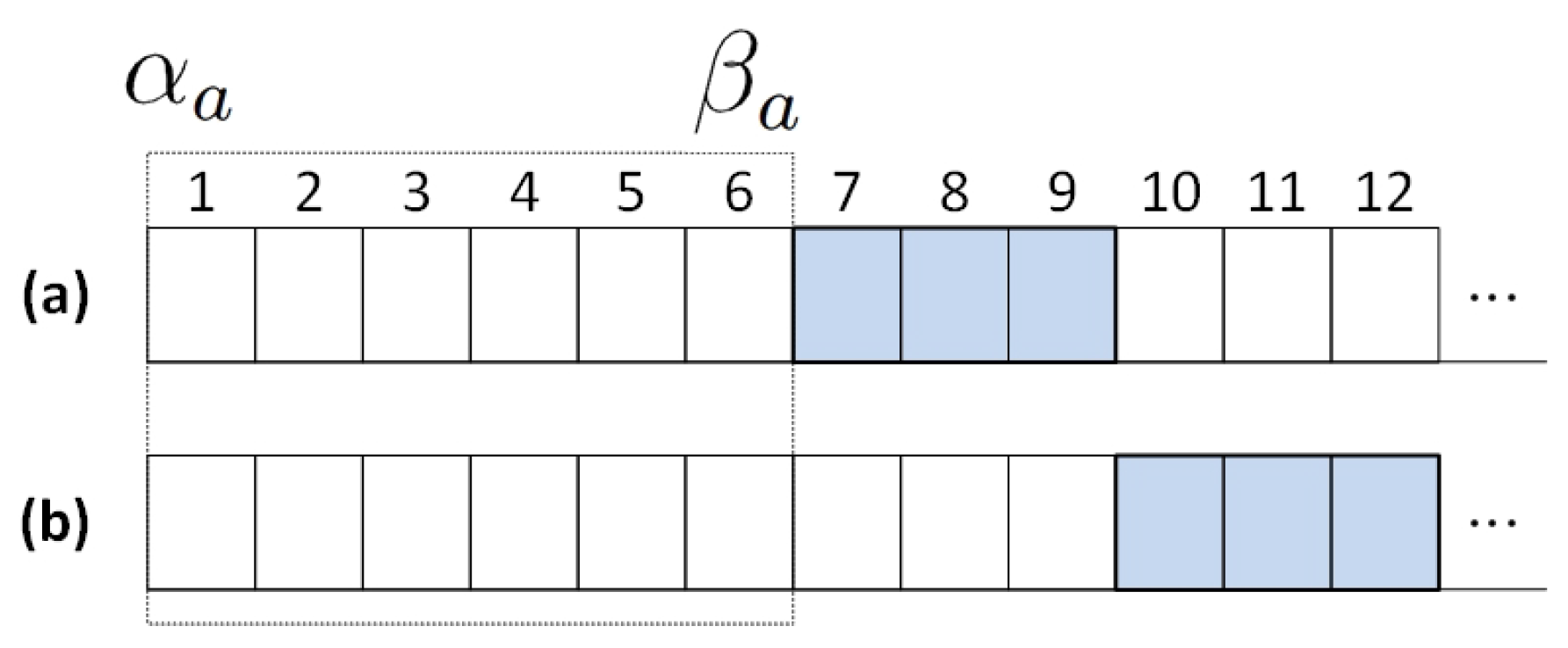
2.3. Objective Function for Semi-Automated Scheduling

In this section, the objective function for semi-automated scheduling is derived. Assume that the preferred start time and end time of each appliance are given by the user. The objective function considers minimization both of the total cost and dissatisfaction (i.e., $B(·)$ and $D(·)$). To fairly consider the two objectives, scaling parameters $\tilde{B}$ and $\tilde{D}$ are introduced since the scales of $B(·)$ and $D(·)$ are different. $\tilde{B}$ is the difference between the expected maximum result (i.e., all appliances are scheduled at the most expensive timeslot) and the expected minimum result (i.e., all appliances are scheduled at the cheapest timeslot) of $B(·)$. $\tilde{D}$ is the difference between the expected maximum result (i.e., all appliances are scheduled at the farthest timeslot from the preferred time) and the expected minimum result (i.e., all appliances are scheduled at farther timeslot from the preferred time) of $D(·)$. The parameter $\omega$ is introduced as a weight factor to combine the two objectives. The objective function of a semi-automated energy scheduling scheme is derived for the residential smart grid demand response system as Equations (11)–(17).

$$\underset{I_a^t}{\mathrm{minimize}}\sum _{t=1}^T\left\{\omega ·\sum _{a\in A}{p}_a^t·I_a^t·E_i^{on}+\right.\left.\frac{(1-\omega )\tilde{B}}{\tilde{D}}·\sum _{a_{\in }\mathcal{A}}\frac{w_i^t·I_a^t}{T_a}\right\}$$

(11)

subject to

$$\begin{array}{ccc}\hfill 0& \le & \omega \le 1\hfill \end{array}$$

(12)

$$\begin{array}{ccc}\hfill \sum _{a_a\in A}{I}_a^t·E_a^{on}& \le & BO\hfill \end{array}$$

(13)

$$\begin{array}{ccc}\hfill \sum _{t=1}^T{I}_a^t& =& T_a\hfill \end{array}$$

(14)

$$\begin{array}{ccc}\hfill \sum _{t={\alpha }_a}^{{\beta }_a}{I}_a^t& \ge & T_a,\forall {\varphi }_a=0\hfill \end{array}$$

(15)

$$\begin{array}{ccc}\hfill \sum _{t=1}^{T-1}{(I_a^t-I_a^{t-1})}^2& \le & 2-I_a^1-I_a^T,\forall {\varphi }_a=1\hfill \end{array}$$

(16)

$$\begin{array}{ccc}\hfill w_a^t& =& \left\{\begin{array}{cc}\hfill {\alpha }_a-t,& t<{\alpha }_a\hfill \\ \hfill 0,& {\alpha }_a\le t<{\beta }_a\hfill \\ \hfill t-{\beta }_a+1,& {\beta }_a\le t.\hfill \end{array}\right.\hfill \end{array}$$

(17)

3. Fully-Automated Energy Scheduling Algorithm

In this section, an algorithm that can automatically search the preferred time for each type of appliance is proposed. The preference time search utilizes appliance-specific usage statistics stored in the database of the demand response architecture. Denote by $u_a^t$ the probability that appliance a will operate at timeslot t, which is expressed as a probability mass function (PMF) based on the usage statistics. Denote by ${\widehat{\alpha }}_a$ the estimated preferred starting time and ${\widehat{\beta }}_a$ the estimated preferred ending time of appliance a. In the later part of this section, the algorithms for searching and estimating preference times ${\widehat{\alpha }}_a$ and ${\widehat{\beta }}_a$ for each appliance type are described.

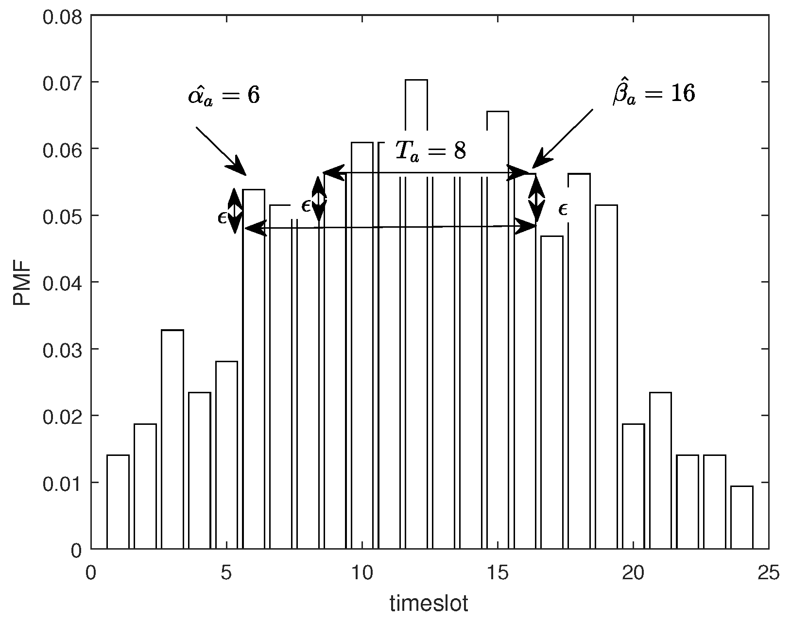
3.1. Searching for the Preference Time for Uncontrollable Appliances

When an uncontrollable appliance a starts, it cannot stop during the determined operation time $T_a$. Therefore, denote by ${\mu }_a^t$ the likelihood that the uncontrollable appliance a starts in timeslot t, which can be obtained as Equation (18).

$${\mu }_a^t=\sum _{j=t}^{T_a-t+1}{u}_a^j.$$

(18)

As mentioned above, uncontrollable appliances should operate exactly at the preferred time. Therefore, the section with the highest frequency is estimated as the preferred time. Figure 6 shows an example distribution for uncontrollable appliances. To estimate the preference time of an uncontrollable appliance, a searching algorithm is proposed in Algorithm 1.

First, set ${\widehat{\alpha }}_a$ and ${\widehat{\beta }}_a$ to the initial timeslot (Lines 1 and 2 in Algorithm 1). Here, i is the index for searching and $Temp$ is the temporary variable to compute the highest frequency (Lines 3 and 4 in Algorithm 1). Then, search the highest frequency section linearly. (Lines 5∼13 in Algorithm 1). If the higher frequency section is found, the ${\widehat{\alpha }}_a$ and ${\widehat{\beta }}_a$ are updated (Lines 7∼11 in Algorithm 1).

Finally, estimate the preferred starting time and preferred ending time as ${\widehat{\alpha }}_a=9$ and ${\widehat{\beta }}_a=16$, respectively.

Algorithm 1: Preference Searching Algorithm for Uncontrollable Appliances

1: $\widehat{{\alpha }_a}\Leftarrow 1$

2: $\widehat{{\beta }_a}\Leftarrow T_a-1$

3: $i\Leftarrow 1$

4: $Temp\Leftarrow 0$

5: while $i+T_a\le T$ do

6:  Calculate ${\mu }_a^i$ by Equation (18)

7:  if $Temp<{\mu }_a^i$ then

8:  $\widehat{{\alpha }_a}\Leftarrow i$

9:  $\widehat{{\beta }_a}\Leftarrow i+T_a-1$

10:  $Temp\Leftarrow {\mu }_a^i$

11: end if

12: $i\Leftarrow i+1$

13: end while

3.2. Searching for the Preference Time for Non-Interruptible Appliances

Non-interruptible appliances cannot stop their operation in the same way uncontrollable appliances can. Non-interruptible appliances, on the other hand, can be scheduled by shifting back and forth. Therefore, the searching algorithm for non-interruptible appliances uses additional techniques compared to the uncontrollable algorithm to find an extra timeslot. To find an additional timeslot, the $ϵ$ searching margin is introduced. If the difference between $u_t^a$ of two adjacent time slots is less than $ϵ$, expand the preference time. Figure 7 shows an example scenario of the searching preferred time for non-interruptible appliances. To estimate the preference time of non-interruptible appliances, a searching algorithm is proposed in Algorithm 2. First, find $\widehat{{\alpha }_a}$ and $\widehat{{\beta }_a}$ using Algorithm 1 (Line 1 in Algorithm 2). In the example scenario, assume that $\widehat{{\alpha }_a}$ and $\widehat{{\beta }_a}$ are 9 and 16, respectively. Next, conduct the following steps iteratively until there are no extensions of the preferred section (Lines 2∼10 in Algorithm 2). If the difference in probability of $\widehat{{\alpha }_a}$ and the adjusted previous timeslot’s probability is less than $ϵ$, update $\widehat{{\alpha }_a}$ (Lines 3 and 4 in Algorithm 2). If the difference in probability of $\widehat{{\beta }_a}$ and the adjusted next timeslot’s probability is less than $ϵ$, update $\widehat{{\beta }_a}$ (Lines 5 and 6 in Algorithm 2). If there are no more extensions of the preferred time section, stop the iterations (Lines 10 and 11 in Algorithm 2). Finally, estimate the preferred starting time and preferred ending time as ${\widehat{\alpha }}_a=6$ and ${\widehat{\beta }}_a=16$, respectively.

Algorithm 2: Preference Searching Algorithm for Uncontrollable Appliances

1: Find $\widehat{{\alpha }_a}$ and $\widehat{{\beta }_a}$ by Algorithm 1

2: while 1 do

3: if $u_a^{\widehat{{\alpha }_a}}-u_a^{\widehat{{\alpha }_a}-1}\le ϵ$ then

4:  $\widehat{{\alpha }_a}\Leftarrow \widehat{{\alpha }_a}-1$

5: else if $u_a^{\widehat{{\beta }_a}}-u_a^{\widehat{{\beta }_a}+1}\le ϵ$ then

6:  $\widehat{{\beta }_a}\Leftarrow {\beta }_a+1$

7: else

8:  break

9: end if

10: end while

3.3. Searching for the Preference Time for Interruptible Appliances

In contrast to the previous two types of appliances, interruptible appliances can be scheduled discretely. Therefore, $\widehat{{\alpha }_a}$ and $\widehat{{\beta }_a}$ have a higher probability of use. To find the estimated preferred time, the $\mathrm{\Gamma }$ threshold parameter is introduced. If the probability is higher than $\mathrm{\Gamma }$, this timeslot is included in the preferred time. Figure 8 shows an example scenario of searching for the preferred time of interruptible appliances. To estimate the preference time of interruptible appliances, a searching algorithm is proposed in Algorithm 3. In the proposed algorithm, the following steps are conducted iteratively (Lines 1∼9 in Algorithm 3). First, find $\widehat{{\alpha }_a}$ and $\widehat{{\beta }_a}$ that have higher probabilities than $\mathrm{\Gamma }$ (Lines 2 and 3 in Algorithm 3). $\widehat{{\alpha }_a}$ can be found by Equation (19).

$$\widehat{{\alpha }_a}=\underset{t}{arg\; min}{y}_a^t,$$

(19)

where

$$y_a^t=\left\{\begin{array}{cc}\infty ,\hfill & \mathrm{if}{u}_a^t>\mathrm{\Gamma }\hfill \\ t,\hfill & \mathrm{otherwise}.\hfill \end{array}\right.$$

$\widehat{{\beta }_a}$ can be computed by Equation (20).

$$\widehat{{\beta }_a}=\underset{t}{arg\; max}{z}_a^t,$$

(20)

where

$$z_a^t=\left\{\begin{array}{cc}0,\hfill & \mathrm{if}{u}_a^t>\mathrm{\Gamma }\hfill \\ t,\hfill & \mathrm{otherwise}.\hfill \end{array}\right.$$

In the example scenario in Figure 8a, $\widehat{{\alpha }_a}$ and $\widehat{{\beta }_a}$ are 12 and 18, respectively. However, these estimated preferred times cannot be used since the operation time $T_a=10$ is larger than the estimated preferred time. Therefore, update $\mathrm{\Gamma }$ by Equation (21) (Lines 4 and 5 in Algorithm 3).

$$\mathrm{\Gamma }\Leftarrow \mathrm{\Gamma }-ϵ.$$

(21)

As shown in Figure 8b, extend the preferred time section by using the updated $\mathrm{\Gamma }$. If the estimated preferred time is larger than the operation time, the search iterations will stop (Lines 6 and 7 in Algorithm 3). Finally, estimate the preferred starting time and preferred ending time as ${\widehat{\alpha }}_a=6$ and ${\widehat{\beta }}_a=18$, respectively.

Algorithm 3: Preference Searching Algorithm for Uncontrollable Appliances

1: while 1 do

2: Update $\widehat{{\alpha }_a}$ by Equation (19)

3: Update $\widehat{{\beta }_a}$ by Equation (20)

4: if $\widehat{{\beta }_a}-\widehat{{\alpha }_a}+1<T_a$ then

5:  Update $\mathrm{\Gamma }$ by Equation (21)

6: else

7:  break

8: end if

9: end while

3.4. Objective Function for Fully-Automated Scheduling

The result of the proposed searching algorithm is used for the objective function of fully-automated scheduling. Therefore, Equations (11)–(17) can be updated to Equations (22)–(28), respectively. The fully-automated scheduling consists of two stages. First, the estimated preferred time of each appliance is found by Algorithms 1–3. Then, optimal scheduling of each appliance is given by the following objective function (Equations (22)–(28)).

$$\underset{I_a^t}{\mathrm{minimize}}\sum _{t=1}^T\left\{\omega ·\sum _{a\in A}{p}_a^t·I_a^t·E_i^{on}+\right.\left.\frac{(1-\omega )\tilde{B}}{\tilde{D}}·\sum _{a_{\in }\mathcal{A}}\frac{w_i^t·I_a^t}{T_a}\right\}$$

(22)

subject to

$$\begin{array}{ccc}\hfill 0& \le & \omega \le 1\hfill \end{array}$$

(23)

$$\begin{array}{ccc}\hfill \sum _{a_a\in A}{I}_a^t·E_a^{on}& \le & BO\hfill \end{array}$$

(24)

$$\begin{array}{ccc}\hfill \sum _{t=1}^T{I}_a^t& =& T_a\hfill \end{array}$$

(25)

$$\begin{array}{ccc}\hfill \sum _{t={\alpha }_a}^{{\beta }_a}{I}_a^t& \ge & T_a,\forall {\varphi }_a=0\hfill \end{array}$$

(26)

$$\begin{array}{ccc}\hfill \sum _{t=1}^{T-1}{(I_a^t-I_a^{t-1})}^2& \le & 2-I_a^1-I_a^T,\forall {\varphi }_a=1\hfill \end{array}$$

(27)

$$\begin{array}{ccc}\hfill w_a^t& =& \left\{\begin{array}{cc}\hfill \widehat{{\alpha }_a}-t,& t<\widehat{{\alpha }_a}\hfill \\ \hfill 0,& \widehat{{\alpha }_a}\le t<\widehat{{\beta }_a}\hfill \\ \hfill t-\widehat{{\beta }_a}+1,& \widehat{{\beta }_a}\le t.\hfill \end{array}\right.\hfill \end{array}$$

(28)

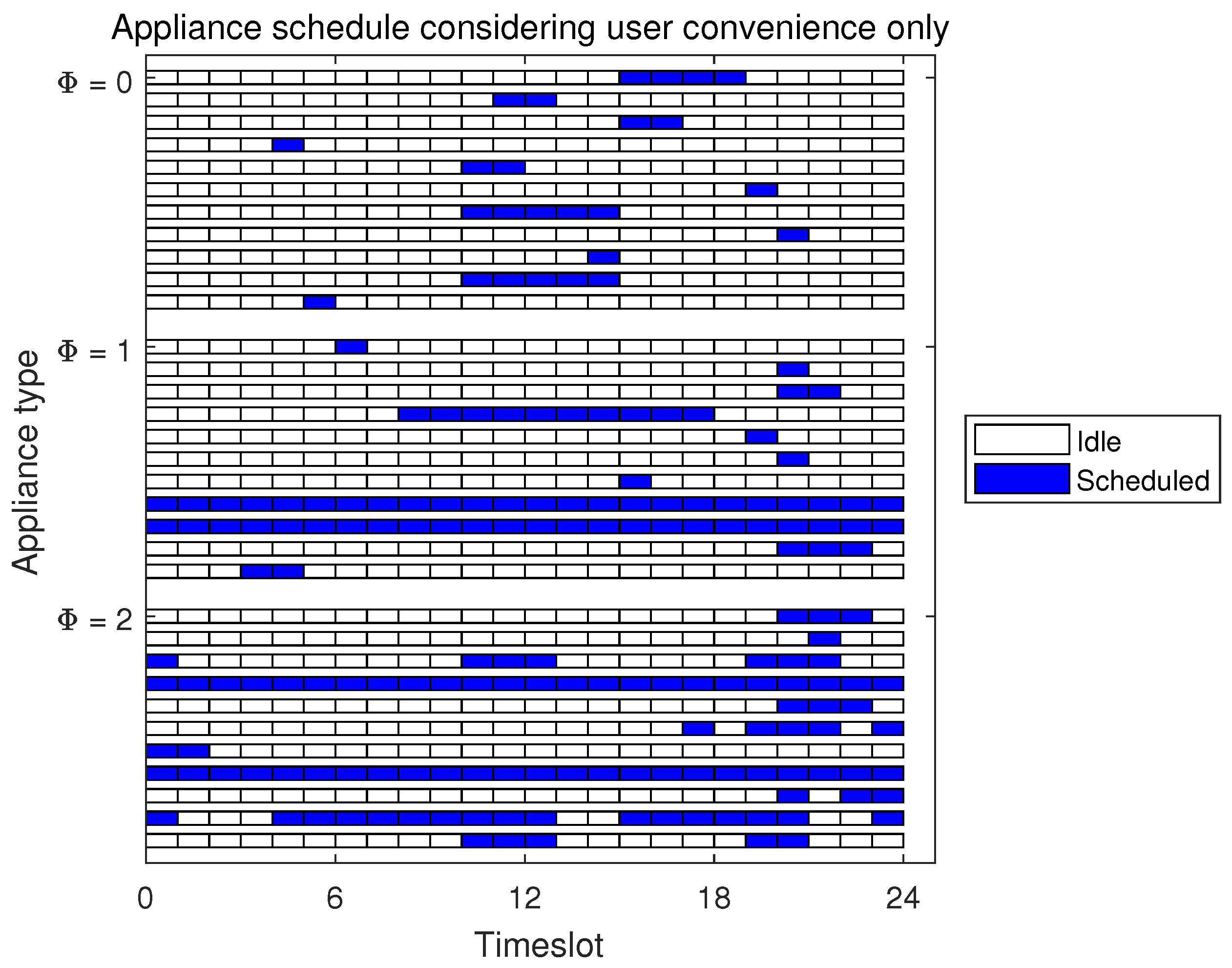
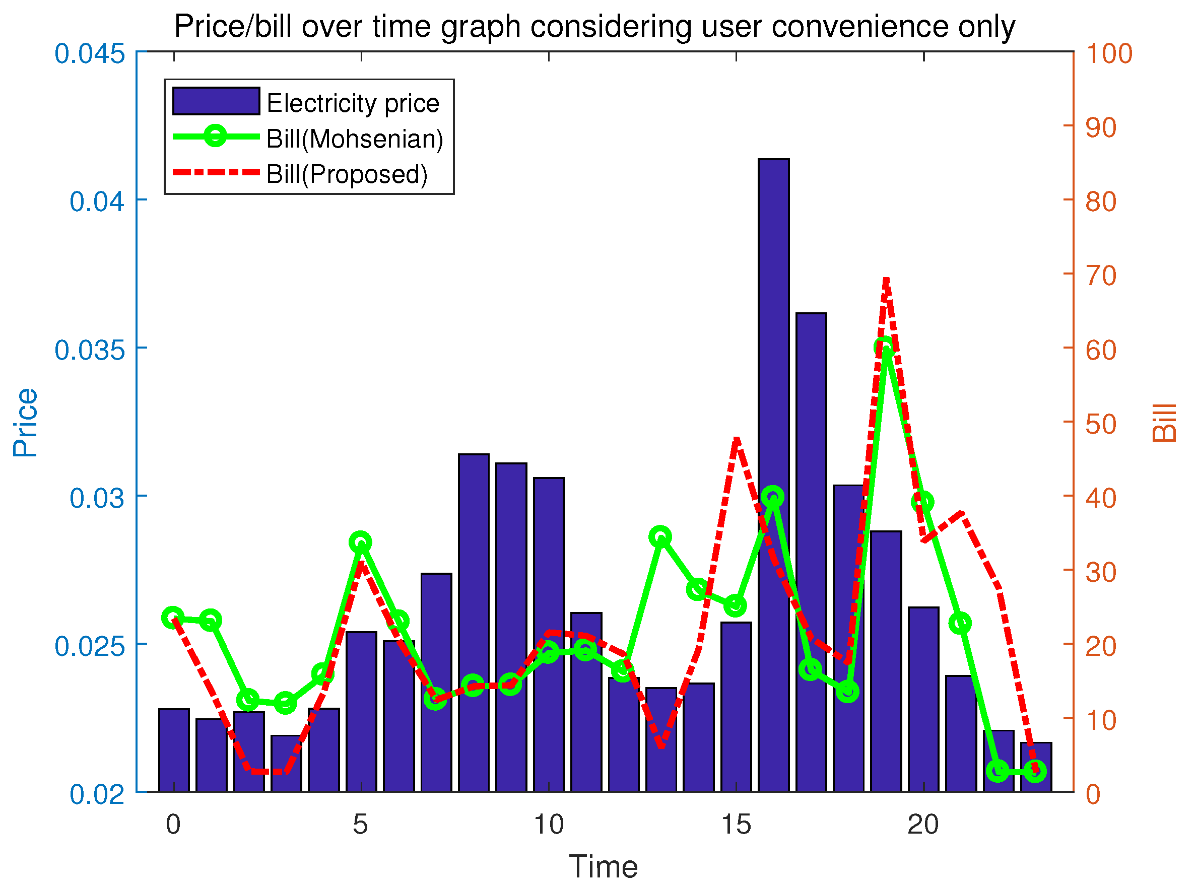
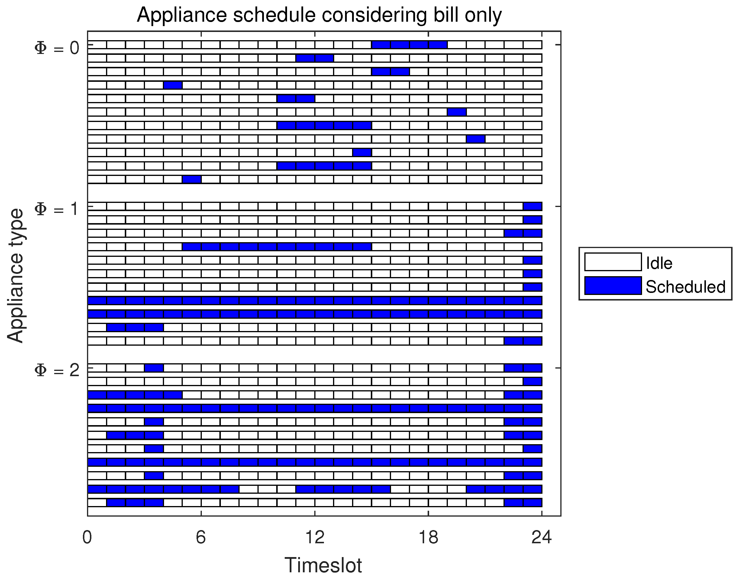
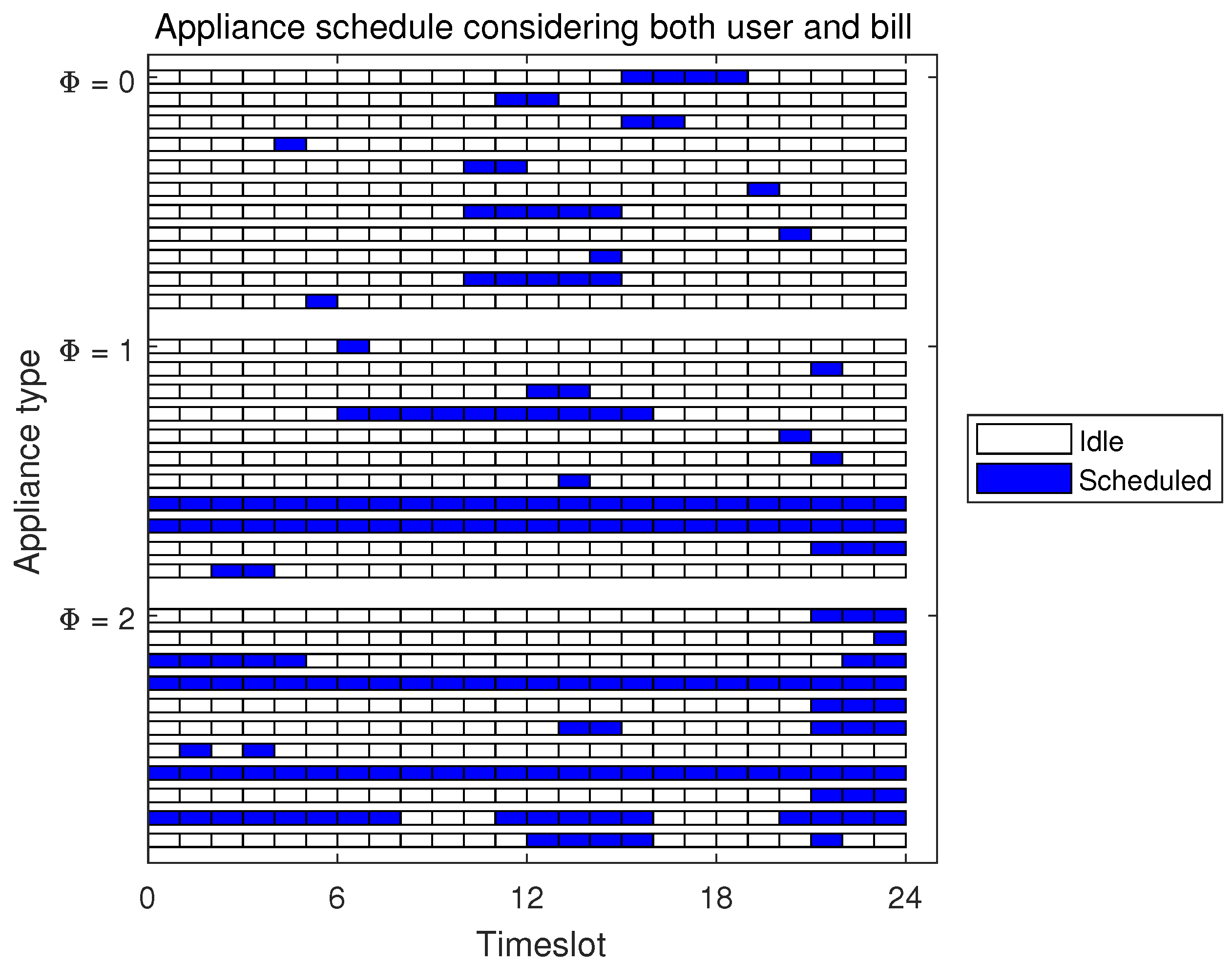
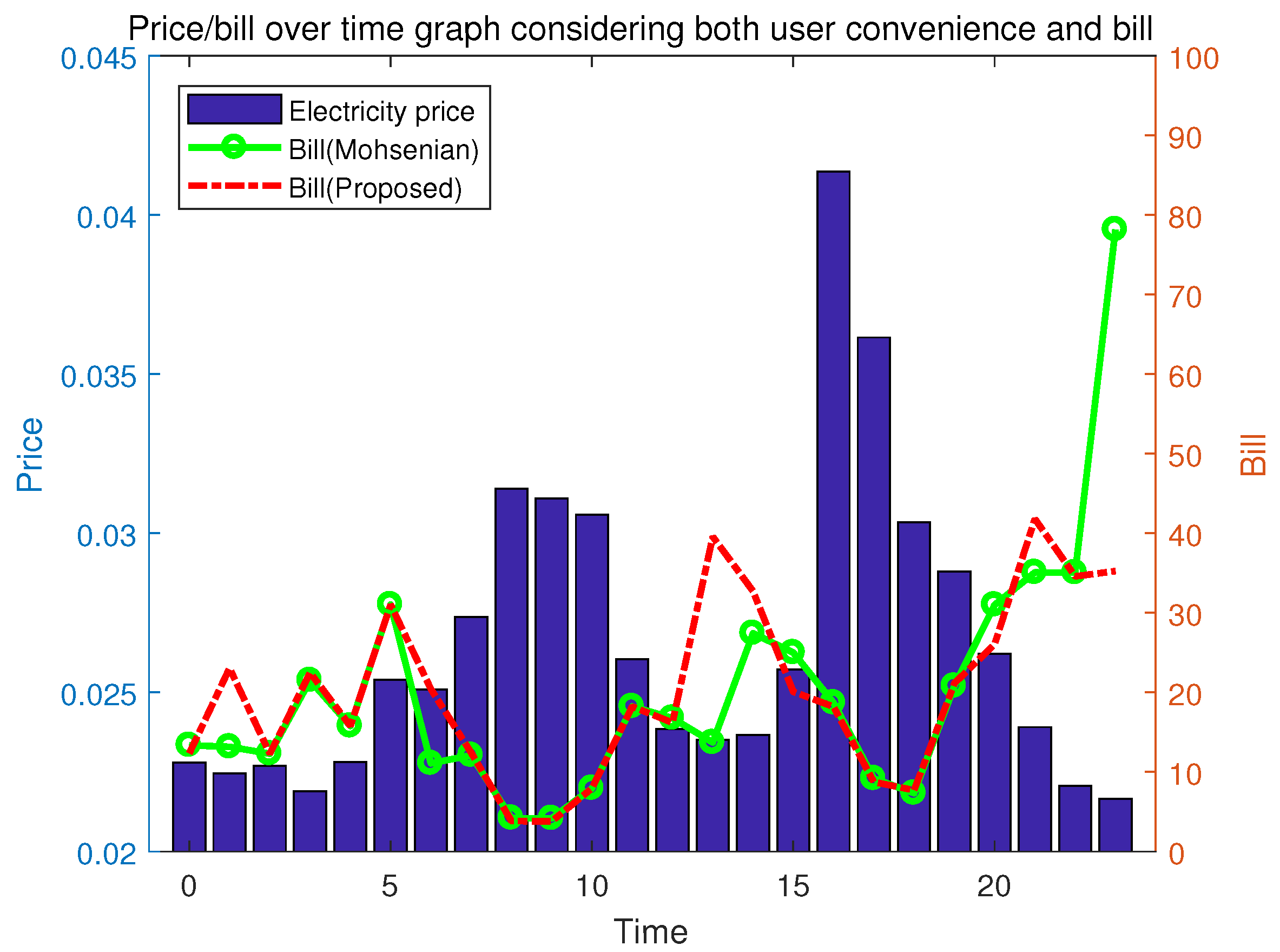
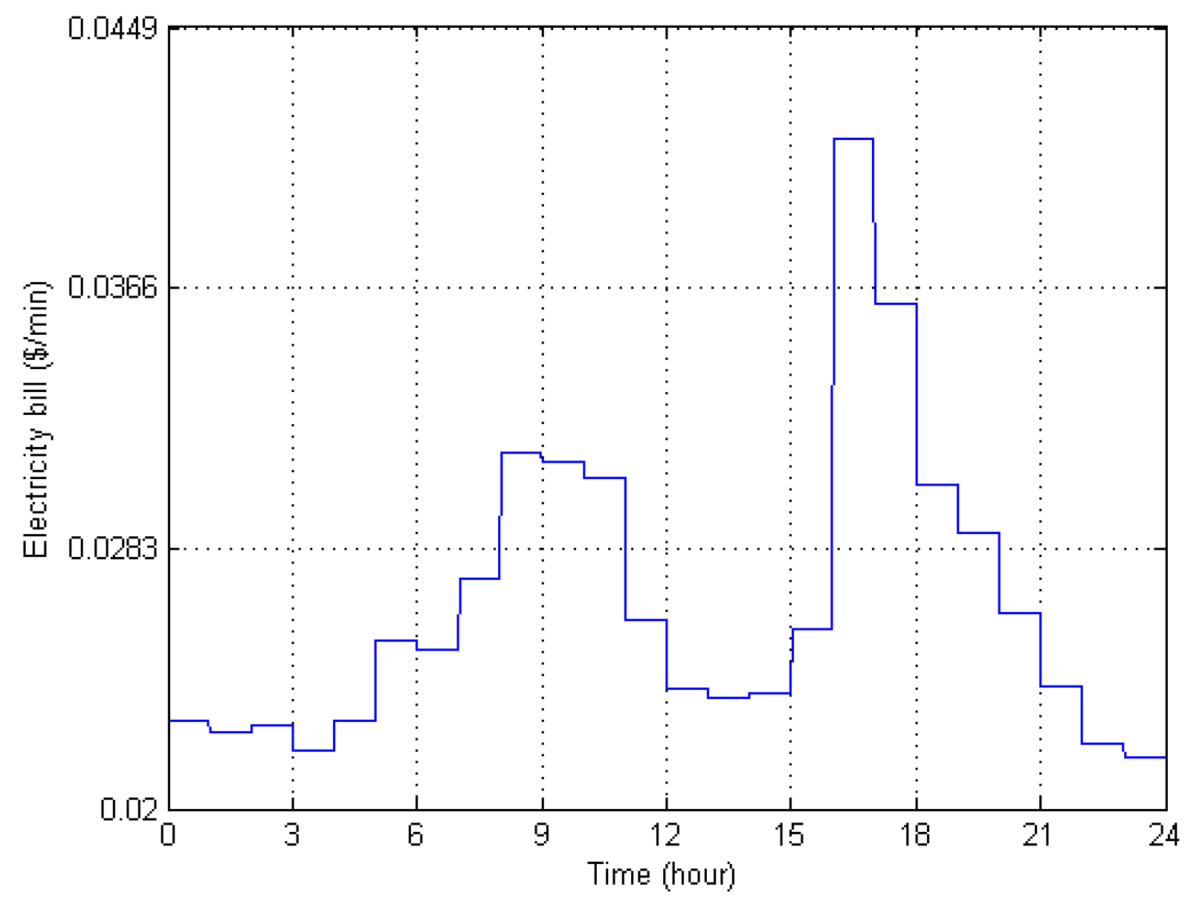
4. Simulation Results

In this section, simulations are conducted to verify the proposed fully-automated demand response algorithm. The simulation is implemented based on the C language, and MOSEK (Version: 7.1.0.54, MOSEK ApS, Copenhagen, Denmark) [21] is used for the optimization interface.

The scenarios include 33 appliances and consider the energy consumption, time duration, and preferred time. The appliances are evenly distributed according to type (i.e., number of $\varphi =0$, number of $\varphi =1$, and number of $\varphi =2$ are all 11).

Table 1. Appliance Profile.

${\mathit{\varphi }}_{\mathit{a}}=0$					${\mathit{\varphi }}_{\mathit{a}}=1$					${\mathit{\varphi }}_{\mathit{a}}=2$
Index ($\mathit{a}$)	${\widehat{\mathbf{\alpha }}}_{\mathit{a}}$	${\widehat{\mathbf{\beta }}}_{\mathit{a}}$	${\mathit{T}}_{\mathit{a}}$	${\mathit{E}}_{\mathit{a}}^{\mathit{on}}$	Index ($\mathit{a}$)	${\widehat{\mathbf{\alpha }}}_{\mathit{a}}$	${\widehat{\mathbf{\alpha }}}_{\mathit{a}}$	${\mathit{T}}_{\mathit{a}}$	${\mathit{E}}_{\mathit{a}}^{\mathit{on}}$	Index ($\mathit{a}$)	${\widehat{\mathbf{\alpha }}}_{\mathit{a}}$	${\widehat{\mathbf{\alpha }}}_{\mathit{a}}$	${\mathit{T}}_{\mathit{a}}$	${\mathit{E}}_{\mathit{a}}^{\mathit{on}}$
1	16	24	4	120	12	6	7	1	360	23	20	24	3	90
2	12	22	2	120	13	20	23	1	74	24	20	24	1	60
3	16	23	2	198	14	11	22	2	24	25	1	24	7	100
4	5	7	1	150	15	7	21	10	12	26	1	24	24	15
5	10	16	2	30	16	17	22	1	12	27	20	24	3	195
6	20	23	1	600	17	19	22	1	198	28	16	24	5	200
7	11	17	5	60	18	14	18	1	900	29	1	8	2	440
8	21	23	1	540	19	1	24	24	84	30	1	24	24	5
9	14	22	1	600	20	1	24	24	18	31	20	24	3	40
10	11	22	5	36	21	20	24	3	500	32	1	24	17	320
11	6	9	1	780	22	1	8	2	44	33	10	22	5	9.1

shows the appliance profile for the simulation. The performance of the proposed algorithm is compared with previous research [11].

Figure 9 shows the scheduling result of each appliance type according to the timeslot if the objective function only considers the user preferred time. As shown in the figure, the uncontrollable and non-interruptable appliances are scheduled in consecutive timeslots. On the other hand, interruptable appliances are scheduled in non-consecutive timeslots. Therefore, the proposed optimization problem works well according to appliance type. Figure 10 shows the electricity bill according to the timeslot if the objective function only considers the user preferred time. As shown in the figure, appliances are scheduled according to their preferences regardless of the real-time pricing for both schemes. However, the scheduling results of the proposed scheme and comparison scheme are a little different. This is because the required operation time of some appliances (such as appliance index 23 or 24) are longer than the preferred section. Therefore, the scheduling of these appliances can belong to any part of their preferred section.

Figure 11 shows the scheduling results of each appliance type according to timeslot if the objective function only considers the electricity bill. As shown in the figure, appliances can be scheduled at 00:00 to 04:00 and 22:00 to 24:00 at the lowest real-time pricing and constraints work well. Figure 12 shows the electricity bill according to timeslot if the objective function only considers electricity bill. In the figure, the electricity consumption is concentrated at 00:00 to 04:00 and 22:00 to 24:00 at the lowest real-time pricing. In contrast to the comparison scheme, the scheduling of the proposed scheme is more concentrated at around 04:00. In the proposed scheme, an appliance can be scheduled earlier than the preferred starting timeslot. Therefore, some appliances have a preferred starting time later than 04:00, and the preferred section larger than 22:00 to 24:00 will be scheduled at around 04:00. However, the comparison scheme cannot be scheduled earlier than the preferred starting timeslot.

Figure 13 shows the scheduling results of each appliance type according to timeslot. Like previous figures, the proposed constraints for appliance type work well. Figure 14 shows the electricity bill according to timeslot if the objective function both considers electricity bill and preferred time. At 22:00 to 24:00, the electricity bill is distributed since the objective function considers the preferred time, unlike in Figure 12. At 15:00, the electricity bill is reduced since the objective function considers the electricity bill, unlike in Figure 10. Therefore, the proposed scheme satisfies both the electricity bill and preferred time. In contrast to the proposed scheme, the comparison scheme is concentrated at 22:00 to 24:00. As mentioned above, the comparison scheme cannot shift to an earlier time. Therefore, the comparison scheme can be concentrated at a later timeslot that has lower real-time pricing.

Table 2. Sum of the electricity bill and the dissatisfaction.

		Only Consider the Electricity Bill	Consider Both the Bill and the Convenience	Only Consider the User Convenience
Proposed Scheme	electricity bill (cents)	479	486	522
	sum of dissatisfaction	103.2	0.6	0
Comparison Scheme	electricity bill (cents)	482	483	520
	sum of dissatisfaction	59.7	40	0

shows the sum of the electricity bill and dissatisfaction. If the optimization problem only considers the electricity bill, the bill will be reduced to 479 cents. However, user dissatisfaction rapidly increases to 103.2. The electricity bill of the comparison scheme is a little expensive and user dissatisfaction is lower than for the proposed scheme if the optimization problem only considers electricity. This is because the proposed scheme can shift to an earlier timeslot. Since this optimization does not consider user dissatisfaction, it found the lowest pricing timeslot. If the optimization considers both the electricity bill and the user convenience (i.e., $\omega =0.5$), the proposed algorithm reduces the electricity bill by 10% when the optimization considers only user convenience. The proposed algorithm can reduce the user dissatisfaction to 0.6. If both the electricity bill and the user convenience are considered, the electricity bill of the proposed scheme is a little more expensive than the comparison scheme, by 2 cents. However, the dissatisfaction of the comparison scheme is larger than the proposed scheme since the comparison scheme can only shift to a later time to reduce the electricity bill. Therefore, the proposed algorithm can satisfy both the electricity bill and user convenience.

5. Conclusions

In this paper, an optimization problem and corresponding algorithms for automated appliance scheduling of residential demand response systems are proposed. For the semi-automated scheduling scheme, the appliance type was categorized according to the controllability, and mathematical formulations that consider the electricity bill and user convenience were proposed. Moreover, scenarios where the user cannot set the appliance preferred time were the main focus, and a fully-automated scheduling algorithm was proposed that can automatically determine the appliance preferred time based on usage statistics. Through intensive simulations, the proposed algorithm was verified to significantly reduce the electricity bill by 10% and satisfy the user convenience. The proposed searching algorithm is sensitive to the values of $ϵ$ and $\tau$. Future research will focus on finding optimal values for $ϵ$ and $\tau$. In addition, the proposed scheme will expand to consider control-wise modeling and multi-scale control approaches in the future.

References

1. Oh, E.; Kwon, Y.; Son, S. A new method for cost-effective demand response strategy for apartment-type factory buildings. Energy Build. 2017, 151, 275–282. [Google Scholar] [CrossRef]
2. Shakeri, M.; Shayestegan, M.; Abunima, H.; Reza, S.M.S.; Akhtaruzzaman, M.; Alamoud, A.R.M.; Sopian, K.; Amin, N. An intelligent system architecture in home energy management systems (HEMS) for efficient demand response in smart grid. Energy Build. 2017, 138, 154–164. [Google Scholar] [CrossRef]
3. Zhou, B.; Yao, F.; Littler, T.; Zhang, H. An electric vehicle dispatch module for demand-side energy participation. Appl. Energy 2016, 177, 464–474. [Google Scholar] [CrossRef]
4. Rubino, L.; Capasso, C.; Veneri, O. Review on plug-in electric vehicle charging architectures integrated with distributed energy sources for sustainable mobility. Appl. Energy 2017, in press. [Google Scholar] [CrossRef]
5. Perez, K.X.; Baldea, M.; Edgar, T.F. Integrated HVAC management and optimal scheduling of smart appliances for community peak load reduction. Energy Build. 2016, 123, 34–40. [Google Scholar] [CrossRef]
6. Paridari, K.; Parisio, A.; Sandberg, H.; Johansson, K.H. Robust Scheduling of Smart Appliances in Active Apartments With User Behavior Uncertainty. IEEE Trans. Autom. Sci. Eng. 2015, 13, 247–259. [Google Scholar] [CrossRef]
7. Cetin, K.S.; Tabares-Velasco, P.C.; Novoselac, A. Appliance daily energy use in new residential buildings: Use profiles and variation in time-of-use. Energy Build. 2014, 84, 716–726. [Google Scholar] [CrossRef]
8. Cetin, K.S. Characterizing large residential appliance peak load reduction potential utilizing a probabilistic approach. Sci. Technol. Built Environ. 2016, 22, 720–732. [Google Scholar] [CrossRef]
9. Chen, Z.; Wu, L.; Fu, Y. Real-Time Price-Based Demand Response Management for Residential Appliances via Stochastic Optimization and Robust Optimization. IEEE Trans. Smart Grid 2012, 3, 1822–1831. [Google Scholar] [CrossRef]
10. Qdr, Q. Benefits of Demand Response in Electricity Markets and Recommendations for Achieving Them; Technical Report; U.S. Department of Energy: Washington, DC, USA, February 2006.
11. Mohsenian-Rad, A.H.; Leon-Garcia, A. Optimal Residential Load Control with Price Prediction in Real-Time Electricity Pricing Environments. IEEE Trans. Smart Grid 2010, 1, 120–133. [Google Scholar] [CrossRef]
12. Yoon, J.H.; Bladick, R.; Novoselac, A. Demand response for residential buildings based on dynamic price of electricity. Energy Build. 2014, 80, 531–541. [Google Scholar] [CrossRef]
13. Ghazvini, M.A.F.; Soares, J.; Abrishambaf, O.; Castro, R.; Vale, Z. Demand response implementation in smart households. Energy Build. 2017, 143, 129–148. [Google Scholar] [CrossRef]
14. Bhattarai, B.P.; Myers, K.S.; Bak-Jensen, B.; Paudyal, S. Multi-Time Scale Control of Demand Flexibility in Smart Distribution Networks. Energies 2017, 10, 37. [Google Scholar] [CrossRef]
15. Yi, P.; Dong, X.; Iwayemi, A.; Zhou, C.; Li, S. Real-Time Opportunistic Scheduling for Residential Demand Response. IEEE Trans. Smart Grid 2013, 4, 227–234. [Google Scholar] [CrossRef]
16. Chen, S.; Sinha, P.; Shroff, N.B. Scheduling Heterogeneous Delay Tolerant Tasks in Smart Grid with Renewable Energy. In Proceedings of the 2012 IEEE 51st IEEE Conference on Decision and Control (CDC), Maui, HI, USA, 10–13 December 2012; pp. 1130–1135. [Google Scholar]
17. Kim, J.; de Dear, R.; Parkinson, T.; Candido, C. Understanding patterns of adaptive comfort behaviour in the Sydney mixed-mode residential context. Energy Build. 2017, 141, 274–283. [Google Scholar] [CrossRef]
18. Ponce, P.; Peffer, T.; Molina, A. Framework for communicating with consumers using an expectation interface in smart thermostats. Energy Build. 2017, 145, 44–56. [Google Scholar] [CrossRef]
19. Tang, S.; Kalavally, V.; Ng, K.Y.; Parkkinen, J. Development of a prototype smart home intelligent lighting control architecture using sensors onboard a mobile computing system. Energy Build. 2017, 138, 368–376. [Google Scholar] [CrossRef]
20. Park, L.; Jang, Y.; Cho, S.; Kim, J. Residential Demand Response for Renewable Energy Resources in Smart Grid Systems. IEEE Trans. Ind. Inform. 2017, in press. [Google Scholar] [CrossRef]
21. MOSEK. Available online: https://www.mosek.com/ (accessed on 5 October 2016).
Figure 1. Concept of the proposed smart grid residential system architecture.
Energies 10 01326 g001
Figure 2. Different state diagrams of (a) uncontrollable, (b) non-interruptable, and (c) interruptable appliances.
Energies 10 01326 g002
Figure 3. Example of time varying prices set by Illinois Power Company on 15 December 2009 [11].
Energies 10 01326 g003
Figure 4. Two different cases of v a if the dissatisfaction is measured by the number of timeslots that are non-overlapping with preferred time.
Energies 10 01326 g004
Figure 5. Two different cases of dissatisfaction degree if the dissatisfaction increases the further away it is from the preferred time.
Energies 10 01326 g005
Figure 6. Example probability mass function (PMF) of an uncontrollable appliance.
Energies 10 01326 g006
Figure 7. Example PMF of a non-interruptible appliance.
Energies 10 01326 g007
Figure 8. Example of PMF of an interruptible appliance.
Energies 10 01326 g008
Figure 9. Scheduling results of appliance vs. timeslot considering only the preferred time.
Energies 10 01326 g009
Figure 10. Electricity bill vs. timeslot considering only the preferred time. The bar is real-time pricing and the plot is the electricity bill.
Energies 10 01326 g010
Figure 11. Scheduling results of appliance vs. timeslot considering only the electricity bill.
Energies 10 01326 g011
Figure 12. Electricity bill vs. timeslot considering only the electricity bill. The bar is real-time pricing and the plot is the electricity bill.
Energies 10 01326 g012
Figure 13. Scheduling results of appliance vs. timeslot if considering both the electricity bill and the preferred time.
Energies 10 01326 g013
Figure 14. Electricity bill vs. timeslot considering both the electricity bill and the preferred time. The bar is real-time pricing and the plot is the electricity bill.
Energies 10 01326 g014