Identification of Critical Transmission Lines in Complex Power Networks

Abstract
1. Introduction
2. Integrated Betweenness to Identify Critical Lines
2.1. The Index of Power Transmission
2.2. The Index of Fault Flow Distribution
2.3. The Index of Influence on System Security
2.4. The Threshold of the Integrated Betweenness
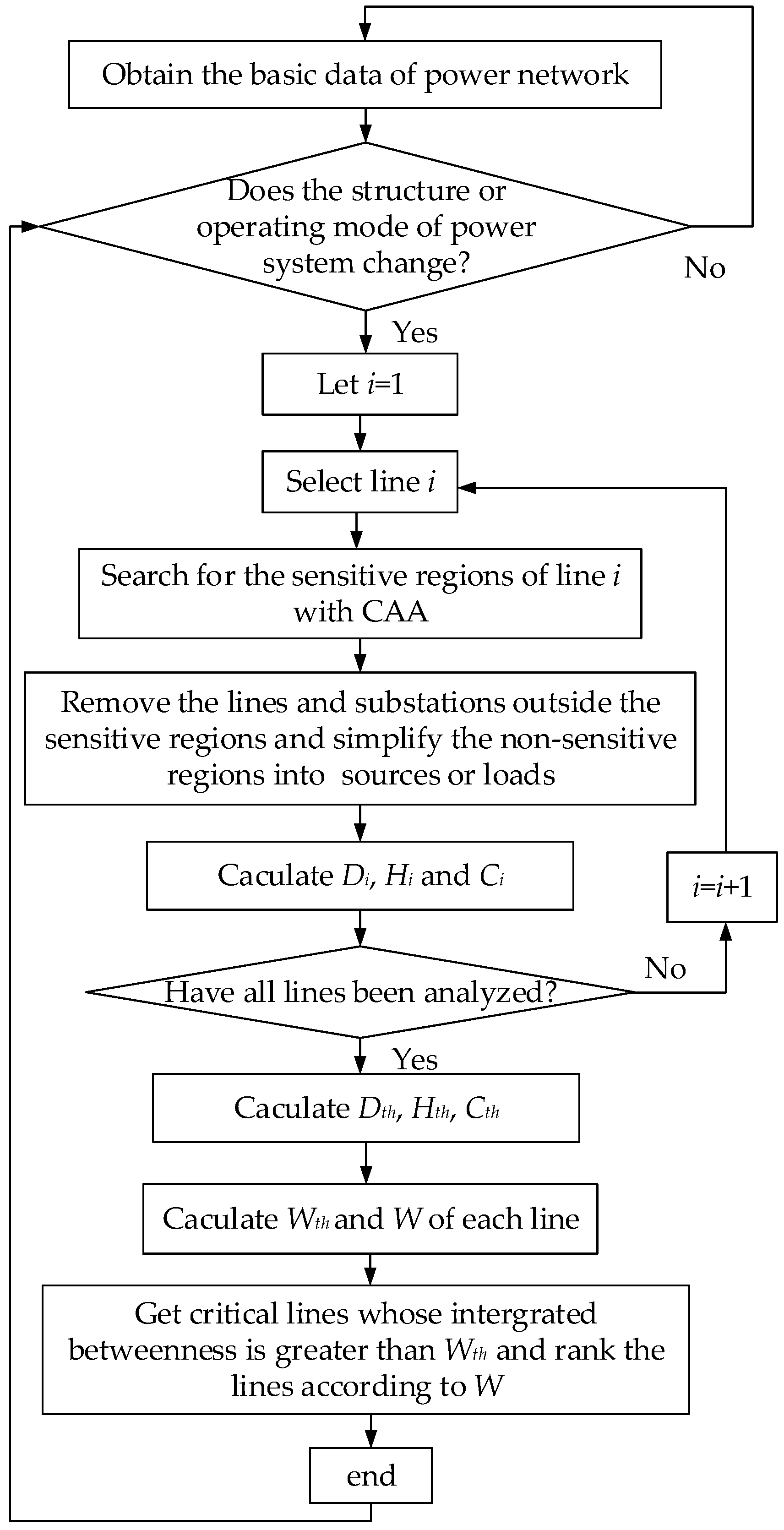
3. Identification Process with Integrated Betweenness and CAA
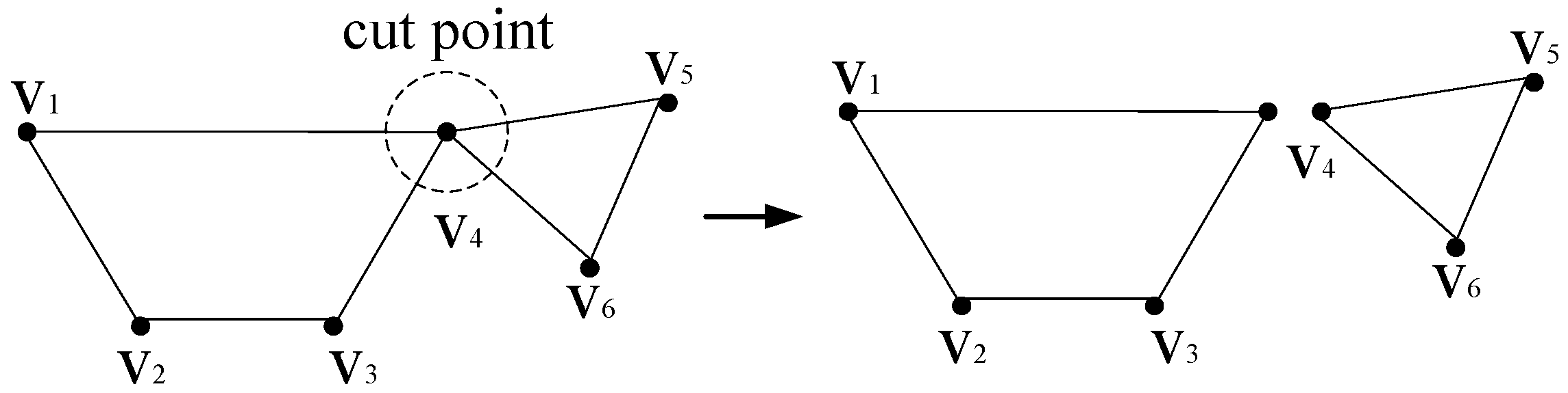
Location of Sensitive Regions with CAA
4. Test Cases
4.1. Location of Sensitive Regions
4.1.1. Location of Sensitive Regions with CAA
4.1.2. Comparison of CAA and Depth-First-Search Method
4.1.3. Accuracy Analysis of the Location Method
4.2. Analysis of Identification Results
4.2.1. Identification Result with Integrated Betweenness and CAA
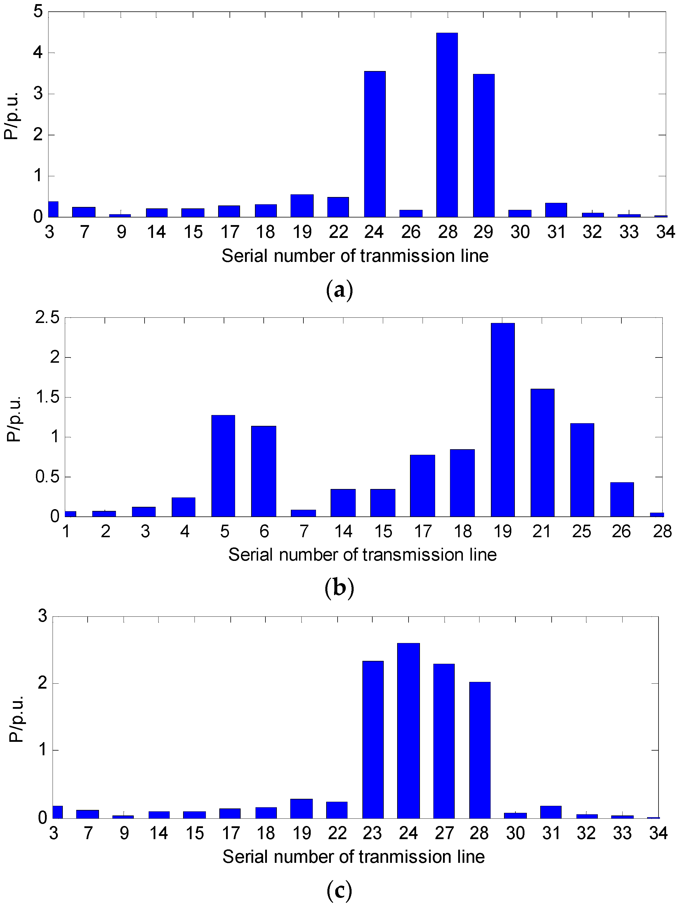
4.2.2. Comparison of Lines with Different Integrated Betweenness
4.3. Comparison of Identification Results
4.4. Extreme Cases and Real-Time Behavior
4.4.1. Extreme Cases
4.4.2. Real-Time Behavior of Power Grids with Different Scales
5. Conclusions
Acknowledgments
Author Contributions
Conflicts of Interest
References
- Hong, S.; Cheng, H.; Zeng, P. An n–k analytic method of composite generation and transmission with interval load. Energies 2017, 10, 168. [Google Scholar] [CrossRef]
- Cai, Y.; Li, Y.; Cao, Y.; Li, W.; Zeng, X. Modeling and impact analysis of interdependent characteristics on cascading failures in smart grids. Int. J. Electr. Power Energy Syst. 2017, 89, 106–114. [Google Scholar] [CrossRef]
- Zeng, K.; Wen, J.; Ma, L.; Cheng, S.; Lu, E.; Wang, N. Fast cut back thermal power plant load rejection and black start field test analysis. Energies 2014, 7, 2740–2760. [Google Scholar] [CrossRef]
- Kosterev, D.N.; Taylor, C.W.; Mittelstadt, W.A. Model validation for the 10 August 1996 WSCC system outage. IEEE Trans. Power Syst. 1999, 14, 967–979. [Google Scholar] [CrossRef]
- Piacenza, J.R.; Proper, S.; Bozorgirad, M.A.; Hoyle, C.; Tumer, I.Y. Robust topology design of complex infrastructure systems. ASCE-ASME J. Risk Uncertain. Eng. Syst. Part B Mech. Eng. 1999, 14, 967–979. [Google Scholar]
- Rampurkar, V.; Pentayya, P.; Mangalvedekar, H.A.; Kazi, F. Cascading failure analysis for Indian power grid. IEEE Trans. Smart Grid 2016, 7, 1951–1960. [Google Scholar] [CrossRef]
- Gao, J.; Liu, X.; Li, D.; Havlin, S. Recent progress on the resilience of complex networks. Energies 2015, 8, 12187–12210. [Google Scholar] [CrossRef]
- Gallos, L.K.; Cohen, R.; Argyrakis, P.; Bunde, A.; Havlin, S. Stability and topology of scale-free networks under attack and defense strategies. Phys. Rev. Lett. 2005, 94, 188701. [Google Scholar] [CrossRef] [PubMed]
- Schneider, C.M.; Moreira, A.A.; Andrade, J.S.; Havlin, S.; Herrmann, H.J. Mitigation of malicious attacks on networks. Proc. Natl. Acad. Sci. USA 2011, 108, 3838–3841. [Google Scholar] [CrossRef] [PubMed]
- Holme, P.; Kim, B.J.; Yoon, C.N. Attack vulnerability of complex networks. Phys. Rev. E 2002, 65, 056109. [Google Scholar] [CrossRef] [PubMed]
- Chen, X.; Sun, K.; Cao, Y.; Wang, S. Identification of vulnerable lines in power grid based on complex network theory. In Proceedings of the Power Engineering-Society General Meeting, Tampa, FL, USA, 24–28 June 2007; pp. 1699–1704. [Google Scholar]
- Dwivedi, A.; Yu, X.; Sokolowski, P. Identifying vulnerable lines in a power network using complex network theory. In Proceedings of the IEEE International Symposium on Industrial Electronics, Seoul, Korea, 5–8 July 2009; pp. 18–23. [Google Scholar]
- Guo, J.; Han, Y.; Guo, C.; Lou, F.; Wang, Y. Modeling and vulnerability analysis of cyber-physical power systems considering network topology and power flow properties. Energies 2017, 10, 87. [Google Scholar] [CrossRef]
- Albert, R.; Albert, I.; Nakarado, G.L. Structural vulnerability of the North American power grid. Phys. Rev. E 2004, 69, 025103. [Google Scholar] [CrossRef] [PubMed]
- Rosas-Casals, M.; Valverde, S.; Sole, R.V. Topological vulnerability of the European power grid under errors and attacks. Int. J. Bifurc. Chaos 2007, 17, 2465–2475. [Google Scholar] [CrossRef]
- Crucitti, P.; Latora, V.; Marchiori, M. A topological analysis of the Italian electric power grid. Phys. A Stat. Mech. Appl. 2004, 338, 92–97. [Google Scholar] [CrossRef]
- Hines, P.; Cotilla-Sanchez, E.; Blumsack, S. Do topological models provide good information about electricity infrastructure vulnerability? Chaos 2010, 20, 033122. [Google Scholar] [CrossRef] [PubMed]
- Cuadra, L.; Salcedo-Sanz, S.; Del Ser, J.; Jimenez-Fernandez, S.; Geem, Z.W. A critical review of robustness in power grids using complex networks concepts. Energies 2015, 8, 9211–9265. [Google Scholar] [CrossRef]
- Xu, L.; Wang, X.; Wang, X. Equivalent admittance small-world model for power system-II. Electric betweenness and vulnerable line identification. In Proceedings of the Asia-Pacific Power and Energy Engineering Conference, Wuhan, China, 27–31 March 2009; pp. 1–4. [Google Scholar]
- Wang, K.; Zhang, B.; Zhang, Z.; Yin, X.; Wang, B. An electrical betweenness approach for vulnerability assessment of power grids considering the capacity of generators and load. Phys. A Stat. Mech. Appl. 2011, 390, 4692–4701. [Google Scholar] [CrossRef]
- Song, H.; Dosano, R.D.; Lee, B. Power grid node and line delta centrality measures for selection of critical lines in terms of blackouts with cascading failures. Int. J. Innov. Comput. Inf. Control 2011, 7, 1321–1330. [Google Scholar]
- Chen, G.; Dong, Z.Y.; Hill, D.J.; Zhang, G.H. An improved model for structural vulnerability analysis of power networks. Phys. A Stat. Mech. Appl. 2009, 388, 4259–4266. [Google Scholar] [CrossRef]
- Bai, H.; Miao, S. Hybrid flow betweenness approach for identification of vulnerable line in power system. IET Gener. Transm. Distrib. 2015, 9, 1324–1331. [Google Scholar] [CrossRef]
- Salim, N.A.; Othman, M.M.; Musirin, I.; Serwan, M.S. Critical system cascading collapse assessment for determining the sensitive transmission lines and severity of total loading conditions. Math. Probl. Eng. 2013, 2013, 965628. [Google Scholar] [CrossRef]
- Wang, A.S.; Luo, Y.; Tu, G.; Liu, P. Vulnerability assessment scheme for power system transmission networks based on the fault chain theory. IEEE Trans. Power Syst. 2011, 26, 442–450. [Google Scholar] [CrossRef]
- Chen, J.; Thorp, J.S.; Dobson, I. Cascading dynamics and mitigation assessment in power system disturbances via a hidden failure model. Int. J. Electr. Power Energy Syst. 2005, 27, 318–326. [Google Scholar] [CrossRef]
- Salim, N.A.; Othman, M.M.; Musirin, I.; Serwan, M.S.; Busan, S. Risk assessment of dynamic system cascading collapse for determining the sensitive transmission lines and severity of total loading conditions. Reliab. Eng. Syst. Saf. 2017, 157, 113–128. [Google Scholar] [CrossRef]
- Kim, S. Accuracy enhancement of mixed power flow analysis using a modified DC model. Energies 2016, 9, 776. [Google Scholar] [CrossRef]
- Zeng, K.; Wen, J.; Cheng, S.; Lu, E.; Wang, N. A critical lines identification algorithm of complex power system. In Proceedings of the Innovative Smart Grid Technologies Conference, Washington, DC, USA, 19–22 February 2014; pp. 1–5. [Google Scholar]
- Zhu, J. Optimal power flow. In Optimization of Power System Operation; Wiley-IEEE Press: Piscataway, NJ, USA, 2015. [Google Scholar]
- Enshaee, A.; Enshaee, P. New reactive power flow tracing and loss allocation algorithms for power grids using matrix calculation. Int. J. Electr. Power. Energy Syst. 2017, 87, 89–98. [Google Scholar] [CrossRef]
- Zhu, D.; Liu, W.; Lv, Q.; Wang, N. Forewarning of cascading failure based on comprehensive entropy of power flow. Appl. Mech. Mater. 2014, 615, 74–79. [Google Scholar] [CrossRef]
- Wang, Q.; McCalley, J.D. Risk and “N − 1” Criteria Coordination for Real-Time Operations. IEEE Trans. Power Syst. 2013, 28, 3505–3506. [Google Scholar] [CrossRef]
- Deka, D.; Backhaus, S.; Chertkov, M. Learning topology of distribution grids using only terminal node measurements. In Proceedings of the IEEE International Conference on Smart Grid Communications, Sydney, Australia, 6–9 November 2016. [Google Scholar]
- Babakmehr, M.; Simoes, M.G.; Wakin, M.B.; Harirchi, F. Compressive sensing-based topology identification for smart grids. IEEE Trans. Ind. Inform. 2016, 12, 532–543. [Google Scholar] [CrossRef]
- Deka, D.; Backhaus, S.; Chertkov, M. Estimating distribution grid topologies: A graphical learning based approach. In Proceedings of the 19th Power Systems Computation Conference, Genova, Italy, 20–24 June 2016. [Google Scholar]
- Deka, D.; Backhaus, S.; Chertkov, M. Learning topology of the power distribution grid with and without missing data. In Proceedings of the European Control Conference, Aalborg, Denmark, 29 June–1 July 2016; pp. 313–320. [Google Scholar]
- Wu, Y.; Li, X. Numerical simulation of the propagation of hydraulic and natural fracture using dijkstra’s algorithm. Energies 2016, 9, 519. [Google Scholar] [CrossRef]
- Chai, D.; Zhang, D. Algorithm and its application to N shortest paths problem. J. Zhejiang Univ. 2002, 5, 61–64. (In Chinese) [Google Scholar]
- Luo, G.; Shi, D.; Chen, J.; Duan, X. Automatic identification of transmission sections based on complex network theory. IET Gener. Transm. Distrib. 2014, 8, 1203–1210. [Google Scholar]
- Berghammer, R.; Hofmann, T. Relational depth-first-search with applications. In Proceedings of the 5th International Seminar on Relational Methods in Computer Science, Valcartier, QC, Canada, 9–14 January 2000; pp. 167–186. [Google Scholar]
- Li, Y.; Su, H. Critical line affecting power system vulnerability under N − k contingency condition. Electr. Power Autom. Equip. 2015, 3, 60–67. (In Chinese) [Google Scholar]
- Yu, X.; Singh, C. A practical approach for integrated power system vulnerability analysis with protection failures. IEEE Trans. Power Syst. 2004, 19, 1811–1820. [Google Scholar] [CrossRef]
- Xie, K.; Zhang, H.; Hu, B.; Cao, K.; Wu, T. Distributed algorithm for power flow of large-scale power systems using the GESP technique. Trans. China Electrotechn. Soc. 2010, 25, 89–95. (In Chinese) [Google Scholar]
- Wu, J. New implementations of wide area monitoring system in power grid of China. In Proceedings of the 2005 IEEE/PES Asia and Pacific Transmission and Distribution Conference and Exhibition, Dalian, China, 14–18 August 2005. [Google Scholar]


| Line | Power Change (MW) | Line | Power Change (MW) | Line | Power Change (MW) | |||
|---|---|---|---|---|---|---|---|---|
| 1 | e34 | 189.7265 | 12 | e13 | 0.584 | 23 | e2 | −0.6828 |
| 2 | e32 | 186.0633 | 13 | e10 | 0.103 | 24 | e14 | −0.6843 |
| 3 | e9 | 2.514 | 14 | e28 | 0.0099 | 25 | e6 | −0.8824 |
| 4 | e7 | 2.4037 | 15 | e29 | 0.0051 | 26 | e25 | −0.8841 |
| 5 | e26 | 2.1787 | 16 | e24 | −0.0082 | 27 | e16 | −1.2161 |
| 6 | e30 | 1.964 | 17 | e27 | −0.0305 | 28 | e12 | −1.3197 |
| 7 | e19 | 1.3781 | 18 | e23 | −0.0328 | 29 | e20 | −1.3791 |
| 8 | e18 | 1.3198 | 19 | e22 | −0.0565 | 30 | e3 | −1.4682 |
| 9 | e21 | 1.2928 | 20 | e8 | −0.0709 | 31 | e4 | −2.1515 |
| 10 | e17 | 1.2161 | 21 | e15 | −0.6759 | 32 | e31 | −2.2252 |
| 11 | e11 | 0.5896 | 22 | e1 | −0.6828 | 33 | e5 | −2.3553 |
| Line | Power Change (MW) | Line | Power Change (MW) | Line | Power Change (MW) | |||
|---|---|---|---|---|---|---|---|---|
| 1 | e19 | 289.8958 | 12 | e31 | −63.5244 | 23 | e10 | −20.1339 |
| 2 | e21 | 288.6156 | 13 | e26 | 63.2027 | 24 | e3 | 15.7069 |
| 3 | e5 | 237.9716 | 14 | e4 | 61.5607 | 25 | e22 | 0.1593 |
| 4 | e25 | 224.116 | 15 | e9 | −48.6027 | 26 | e23 | 0.0991 |
| 5 | e6 | 222.5013 | 16 | e1 | 45.4289 | 27 | e27 | 0.0972 |
| 6 | e8 | −208.162 | 17 | e2 | 45.4289 | 28 | e28 | −0.033 |
| 7 | e18 | 81.8674 | 18 | e15 | 45.2833 | 29 | e33 | 0.0229 |
| 8 | e12 | −81.6569 | 19 | e14 | 45.1093 | 30 | e32 | −0.0216 |
| 9 | e17 | 75.1401 | 20 | e7 | −28.4259 | 31 | e34 | −0.0211 |
| 10 | e16 | −75.1401 | 21 | e11 | −25.1939 | 32 | e24 | 0.0187 |
| 11 | e30 | −63.6899 | 22 | e13 | −25.0956 | 33 | e29 | −0.0182 |
| Line | Index | W | Line | Index | W | ||||||
|---|---|---|---|---|---|---|---|---|---|---|---|
| D | H | C | D | H | C | ||||||
| 1 | e27 | 0.7439 | 1 | 0.7975 | 2.5415 | 18 | e18 | 0.0749 | 0.3855 | 0.0893 | 0.5497 |
| 2 | e3 | 1 | 0.4868 | 0.8282 | 2.3150 | 19 | e17 | 0.0845 | 0.4046 | 0.0590 | 0.5482 |
| 3 | e20 | 0.6249 | 0.3874 | 0.9302 | 1.9426 | 20 | e1 | 0.0454 | 0.1499 | 0.2332 | 0.4286 |
| 4 | e31 | 0.5744 | 0.3437 | 1 | 1.9182 | 21 | e2 | 0.0454 | 0.1499 | 0.2332 | 0.4286 |
| 5 | e4 | 0.4285 | 0.3214 | 0.8308 | 1.5809 | 22 | e13 | 0.0473 | 0.2791 | 0.0370 | 0.3636 |
| 6 | e23 | 0.2676 | 0.5499 | 0.4379 | 1.2555 | 23 | e30 | 0.0042 | 0.0887 | 0.2409 | 0.3339 |
| 7 | e34 | 0.67893 | 0.3823 | 0.0890 | 1.1502 | 24 | e5 | 0.0681 | 0.1215 | 0.0919 | 0.2816 |
| 8 | e12 | 0.3574 | 0.4769 | 0.1919 | 1.0263 | 25 | e33 | 0 | 0.2001 | 0.0626 | 0.2628 |
| 9 | e21 | 0.1928 | 0.2595 | 0.5214 | 0.9738 | 26 | e7 | 0.0397 | 0.1927 | 0.0276 | 0.2601 |
| 10 | e29 | 0.0523 | 0.5406 | 0.3566 | 0.9495 | 27 | e32 | 0 | 0.1421 | 0.0322 | 0.1743 |
| 11 | e11 | 0.1849 | 0.6203 | 0.0867 | 0.8919 | 28 | e6 | 0.0517 | 0.0467 | 0.0556 | 0.1541 |
| 12 | e16 | 0.1981 | 0.4950 | 0.1285 | 0.8218 | 29 | e24 | 0.0334 | 0.0832 | 0.0055 | 0.1222 |
| 13 | e22 | 0.1972 | 0.5363 | 0.0419 | 0.7755 | 30 | e28 | 0.0329 | 0.0760 | 0.0049 | 0.1139 |
| 14 | e8 | 0.1445 | 0.3247 | 0.2794 | 0.7488 | 31 | e14 | 0.0698 | 0.0247 | 0.0047 | 0.0993 |
| 15 | e9 | 0.0232 | 0.6239 | 0.0892 | 0.7364 | 32 | e15 | 0.0698 | 0.0247 | 0.0047 | 0.0993 |
| 16 | e10 | 0.0957 | 0.4873 | 0.0881 | 0.6711 | 33 | e19 | 0.0363 | 0.0231 | 0.0013 | 0.0607 |
| 17 | e25 | 0.0434 | 0.2404 | 0.3199 | 0.6038 | 34 | e26 | 0.0014 | 0.0190 | 0.0149 | 0.0354 |
| Line | W | Line | W | Line | W | Line | W | Line | W |
|---|---|---|---|---|---|---|---|---|---|
| e1 | 0.2489 | e8 | 0.5680 | e15 | 0.0955 | e22 | 1.2320 | e29 | 0.6616 |
| e2 | 0.2489 | e9 | 0.6824 | e16 | 1.0743 | e23 | 0.9019 | e30 | 0.1394 |
| e3 | 1.6463 | e10 | 0.6000 | e17 | 0.5979 | e24 | 0.1177 | e31 | 1.1108 |
| e4 | 0.9140 | e11 | 0.8219 | e18 | 0.4032 | e25 | 0.3507 | e32 | 0.1483 |
| e5 | 0.2073 | e12 | 0.9458 | e19 | 0.0597 | e26 | 0.0234 | e33 | 0.2122 |
| e6 | 0.1092 | e13 | 0.3337 | e20 | 1.1916 | e27 | 1.8976 | e34 | 1.0783 |
| e7 | 0.2291 | e14 | 0.0955 | e21 | 0.5660 | e28 | 0.1099 |
| Line | W | Line | W | Line | W | Line | W | Line | W |
|---|---|---|---|---|---|---|---|---|---|
| e1 | 0.4372 | e8 | 0.7937 | e15 | 0.0993 | e22 | 1.2659 | e29 | 0.9495 |
| e2 | 0.4372 | e9 | 0.7544 | e16 | 1.1781 | e23 | 1.2555 | e30 | 0.3339 |
| e3 | 2.3150 | e10 | 0.6711 | e17 | 0.6456 | e24 | 0.1222 | e31 | 1.9182 |
| e4 | 1.5848 | e11 | 0.8919 | e18 | 0.4753 | e25 | 0.6090 | e32 | 0.1743 |
| e5 | 0.2816 | e12 | 1.1008 | e19 | 0.0607 | e26 | 0.03546 | e33 | 0.2628 |
| e6 | 0.1541 | e13 | 0.3636 | e20 | 1.9426 | e27 | 2.5415 | e34 | 1.1502 |
| e7 | 0.2514 | e14 | 0.0993 | e21 | 0.9870 | e28 | 0.1139 |
| Test System | Number of Buses | Computation Time (s) |
|---|---|---|
| IEEE39 | 39 | 0.061 |
| IEEE118 | 118 | 0.319 |
| SYN472 | 472 | 1.285 |
| SYN1062 | 1062 | 2.891 |
| SYN3000 | 3000 | 7.639 |
| SYN7680 | 7680 | 32.268 |
| SYN12000 | 12,000 | 73.512 |
© 2017 by the authors. Licensee MDPI, Basel, Switzerland. This article is an open access article distributed under the terms and conditions of the Creative Commons Attribution (CC BY) license (http://creativecommons.org/licenses/by/4.0/).
Share and Cite
Wang, Z.; He, J.; Nechifor, A.; Zhang, D.; Crossley, P. Identification of Critical Transmission Lines in Complex Power Networks. Energies 2017, 10, 1294. https://doi.org/10.3390/en10091294
Wang Z, He J, Nechifor A, Zhang D, Crossley P. Identification of Critical Transmission Lines in Complex Power Networks. Energies. 2017; 10(9):1294. https://doi.org/10.3390/en10091294
Chicago/Turabian StyleWang, Ziqi, Jinghan He, Alexandru Nechifor, Dahai Zhang, and Peter Crossley. 2017. "Identification of Critical Transmission Lines in Complex Power Networks" Energies 10, no. 9: 1294. https://doi.org/10.3390/en10091294
APA StyleWang, Z., He, J., Nechifor, A., Zhang, D., & Crossley, P. (2017). Identification of Critical Transmission Lines in Complex Power Networks. Energies, 10(9), 1294. https://doi.org/10.3390/en10091294