1. Introduction
Small electricity consumers, apart from the regulations that ban them from participation in the pool market, are usually unwilling to participate in volatile pool markets. They are unprepared for forecasting the market price and even predicting their own load forecast.
Retail electricity providers (REPs) bridge the gap between wholesale electricity markets and end-users. In addition to the forward contracts, they procure part of the demand of their customers through the pool market [
1]. Thus they have an intermediary role in electricity markets [
2]. The main challenge of REPs is buying power on the wholesale market at volatile prices and selling it to the clients at the retail level at fixed agreed rates [
2]. Price spikes are a source of great concern for the REPs, who need to buy power at spot prices to fulfill their obligations to their clients [
3]. The REP should handle the uncertainties it faces while buying and selling electricity [
1]. Usually, the REPs do not have enough information about the distribution and behaviors of uncertain parameters such as market price and load demand [
4]. Robust optimization models are proposed for decision-making frameworks that are affected by uncertainty, where the decision-maker lacks the full information.
1.1. Motivation
Liberalization reforms in retail electricity markets have facilitated the entrance of smaller companies into the retailing businesses. These companies are exposed to financial risks, and surviving in the uncertain environment of electricity markets requires special strategies. Smart grid deployment has enabled new approaches for them to deal with these challenges. They can procure the energy requirements of their clients from other sources than the pool market. Customers can be served from the DG (distributed generation) units and the energy storage systems (ESS) that the REP owns in their distribution network.
Small REPs that have recently joined the retailing business are more prone to have less information about the market’s behavior and their new customers [
4]. Therefore, they need some computational tools to make them robust against the variations of uncertain inputs and to improve their chance to be more competitive [
4]. Modeling the pool price uncertainty is essential for the REPs because a serious challenge for retailing businesses in electricity markets is buying electricity at variable prices in the pool market and selling it at specified rates to the end-users [
2]. Their main cost in the pool market is unknown due to the variations in the price [
2].
1.2. Objectives
The objective of this paper is to determine the optimal hourly retail sale prices for the next day. The purpose is to provide effective computational tools for asset-light REPs to make them robust against the variations that exist in the wholesale market. Within the developed framework, the REP can determine the dynamic retail prices and optimally schedule the bilateral contracts at each node in the distribution network. Uncertainty of wholesale market prices is taken into account with a robust optimization model, in which, instead of predicted prices, the upper and lower limits of the pool prices are considered. In the robust optimization model, the decision-maker can rely on the upper and lower bounds of the market price, instead of fully trusting a single forecasted price profile, which is usually different from the actual values [
2]. In contrast to the stochastic programming method, the robust optimization technique exhibits a low computational burden and effective results [
5].
1.3. Literature Review
Most of the existing models in the literature use stochastic programming to model the uncertainties, which is computationally expensive and depends on the probability density function of the uncertain inputs [
4]. Computational burdens are important for decision-makers, especially for smaller companies with limited resources.
REP companies can determine the optimal selling price to their customers and the energy-supply strategy to cover the costs and ensure an acceptable profit with the model proposed in [
6]. In this model, the risk preferences of the REP Company are taken into account. Risk-averse companies prefer lower risk levels to hedge their financial losses in the market, and the strategies of the risk-taker companies generally entail more risk in the hope of obtaining higher profits [
6].
REPs’ time of use (TOU) selling price of electricity for a medium-term period with a lead time of one month to a few months is determined with a stochastic-based decision-making framework in [
7]. In the proposed model, the elastic behavior of customers to different blocks of TOU rates is considered. The REPs in this model can also use a portfolio of different options to procure demand and hedge against the risk.
The optimal charging of electric vehicle (EV) loads based on TOU rates is the main decision variable of the REP company modeled in [
8]. The only source of uncertainty considered in this model is the EVs’ fleet demand. The uncertainty of wholesale market prices is not included in this model. The REPs can use multiple sources such as bilateral contracts and call-options to provide energy for their clients. They can also sell the surplus self-produced power to the market.
A risk-constrained stochastic programming framework is proposed in [
1] determine the forward contracting decisions and TOU prices within a yearly framework. The REP maximizes the profit for a specific risk level of profit changes [
1].
The elastic behavior of consumers toward financial incentives is considered in [
9,
10] to determine the incentive plan that can be offered to end-users to reduce their consumption. However, the mixed-integer nonlinear decision-making framework of these models might cause convergence issues.
The effective application of robust optimization models to the retailers’ decision-making models has been recently reported in the literature. The optimal bidding strategy of a risk-averse price-taker retailer is constructed with a robust optimization approach in [
2]. The retail rates are fixed and considered an input in this model. The scheduling horizon is four weeks, and the curves that they obtain provide the required information for the retail company to bid for the customers’ demand on the market.
A scenario-based stochastic programming model is proposed in [
11] to solve the selling price determination problem of an asset-light REP. They found out that the selling price determination based on real-time pricing (RTP) enables them to earn higher profits, compared to fixed price tariffs and time-of-use pricing methods.
The problem of dispatching and energy pricing by a smart grid retailer is addressed in [
12] through a two-stage two-level model. The main source of uncertainty in the model was the market price uncertainty. In this model, the determination of the offering prices is done in a separate level from determining the operating details of the storage units and storage contracts.
A robust risk-hedging tool for the virtual power player (VPP) self-scheduling is proposed in [
13]. The VPP in this model is composed of different types of DG units and does the retailing business itself. This risk-hedging tool guarantees that a minimum level of critical profit and bilateral contract fulfillment for VPPs will be obtained, based on the assumption that the realized market prices are deviated in a trust region [
13].
1.4. Contributions
The selling price determination for a short-term horizon is overlooked in the literature. The proposed model enables the REPs to offer dynamic retail rates for the next day. It also formulates a self-scheduling problem for a REP. Most of the models proposed in the literature for self-generation scheduling are performed from the perspective of power generation companies or market operators. However, in future, the retail companies, especially those without integration with the generation-side, can widely employ these light resources in the distribution network to manage their payoff [
14].
In this paper, a robust optimization model that can be used by REPs for short-term decision-making in electricity markets is proposed and developed. With this model, they can determine the purchases from the pool market and the optimal operation of their resources and the optimal participation in bilateral contracts. The contributions of this paper are:
It considers the retail rates as variables for the short-term scheduling horizon. Dynamic sale prices are determined for different customer groups based on their short run price elasticities. The elastic behavior of end-users towards the blocks of real-time prices is taken into account in the model. Retail rates can be calculated for a lead time of one day.
The model considers involvement in bilateral contracts and the pool market to determine the optimal electricity procurement policy, without knowing the precise values of price and demand.
It enables the REPs to tune their level of conservatism through a flexible decision-making framework. The optimal solutions are immune against the forecast errors to some controlled extent.
1.5. Paper Organization
This paper is organized as follows. The revenue function of the REP and the cost function for considering each risk hedging strategy is presented in
Section 2. The concept of robust optimization and the robust counterpart of this problem are introduced in
Section 3. Numerical studies and the associated discussions are provided in
Section 4. Finally, the concluding remarks are presented in
Section 5.
2. Problem Formulation
The main objective of the REP in the short-term horizon is to maximize the expected profit. The REP can benefit from a set of strategies to manage the expected payoff and to control the risk of financial losses in the market. A wide range of strategies can be employed by them. For instance, they can offer dynamic tariffs to their eligible clients, those equipped with smart meters. Another possibility for them is to employ the light physical assets that they may own in the distribution network, namely the DGs and the ESSs. Therefore, setting the tariffs and finding the optimal hourly schedule of the resources for the next day should be completed at this stage. The main assumptions of the proposed model are as follows:
Customers are equipped with smart meters. Thus the dynamic prices offered by the REP can be employed at the end-users’ points.
REPs have sufficient data about the DG units’ cost functions, bilateral contracts, and the price elasticity of demand for each time period.
Customers behave elastically in the short term. They are assumed to be flexible. If the price increases, they shift demand to periods with lower prices.
Each node refers to zones with similar market prices. Therefore, this model can be used by REPs that serve loads at several distribution networks.
The expected payoff of the REP is calculated based on price and load demand forecasts rather than the actual values of these inputs.
The dynamic prices for residential retail consumers can be used to control the consumption of controllable appliances such as electric vehicles, heat pumps, and electric water heaters [
15]. The consumers also require a specialized control system, which is usually known as a home energy management system, to make optimal decisions for changing the demand profile. The main inputs of the home energy management system, apart from the built-in parameters of the controllable devices, are the price signals that the REPs send to the end-users.
The inputs of the model are the characteristics of the DG and ESS units, the forecasted price of the market, and the demand of each load group. By linearizing the non-linear components of the optimization problem, the optimized results are obtained more efficiently. The optimal value of the objective function in this situation is also the global optimum of the problem. The expected profit of REPs is the difference between the revenue and the costs, where the revenue is derived from selling energy to the customers at retail rates (
) and the costs illustrate the cost of energy procurement from different sources. The revenue function of a REP during the scheduling horizon is shown by Equation (1). For companies with pure retailing portfolios in the wholesale market, the only origin of revenue is selling electricity to the end-users. The retail rates are the time-varying prices for each customer group. The demand of each customer group (
is also considered a variable that changes with regard to the dynamic rates of the electricity.
The hourly retail rates can be considered a variable for price-sensitive retail consumers. Consumers adjust their consumption in response to price signals sent from the REPs [
16]. In this model, the price signals are the dynamic retail rates. Dynamic rates are different from the wholesale market price and are determined by the retailing entity one day in advance. Demand is also considered a function of the retail rates offered to customers. The predicted base load profile (
) for each customer group represents the consumption of each group when DR programs are not applied. Another important term is the percentage of demand flexibility at each time period, which has leading role in determining the retail rates. Within this range, the customers react to price [
17]. This term can also reflect the range of price changes when the demand functions are used to represent the price elasticity of the end-users.
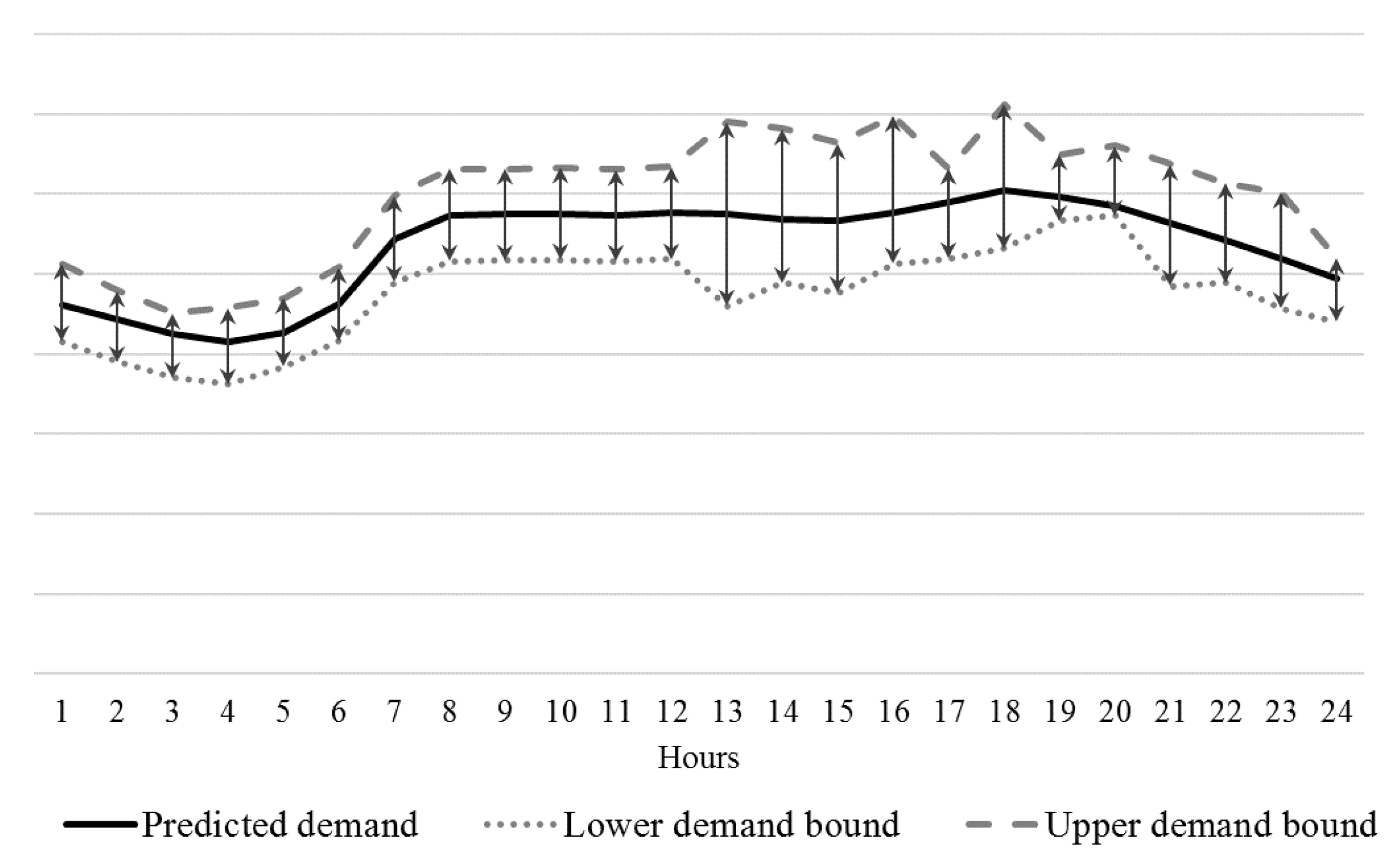
Figure 1 shows a typical forecasted demand profile by the REP. This graph also shows the flexibilities of the demand profile. As the demand is considered price elastic, it is expected that the demand changes with the changes of the retail rates. The REP expects that the consumption can increase and decrease within the specified bound.
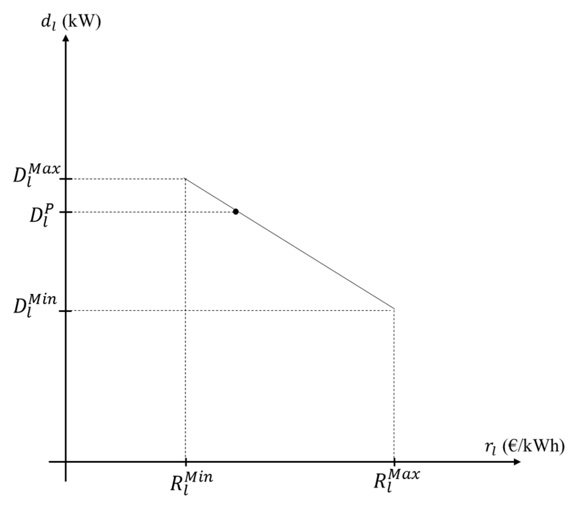
The demand function for one time period is shown in
Figure 2. This is a linear representation of the original demand function in the interval in which the REP expects fluctuation of the demand. The REP has estimated the demand function in a range, which is limited with the lower (
) and upper (
) demand bounds, and incorporates the predicted base load demand (
) for each customer group.
Consumers can reflect different elasticity behavior during the day; therefore this linear representation () varies for each customer group and for each time period (i.e., ).
The sensitivity of clients with regard to price changes is called the price elasticity of demand [
17]. The price elasticity (
ε) of electricity is the percentage by which energy consumption changes due to one percentage of price change Equation (2) [
17]. In this model, price changes refer to the changes of dynamic rates that are offered to the consumers. The knowledge of short run price elasticities is important for the REPs in dynamic pricing [
17]. It is assumed that the REPs can estimate the elasticity of their customer groups at a certain range around the predicted demand [
17].
The short run price elasticity of demand is usually referred to as the immediate behavioral changes of the electricity consumers in response to price changes. This change can be made by the consumer or through a home energy management system. When the prices increase, the customers shift the part of their load that is controllable. The lower demand bound represents the firm demand, which is the uncontrollable load that cannot respond to price changes.
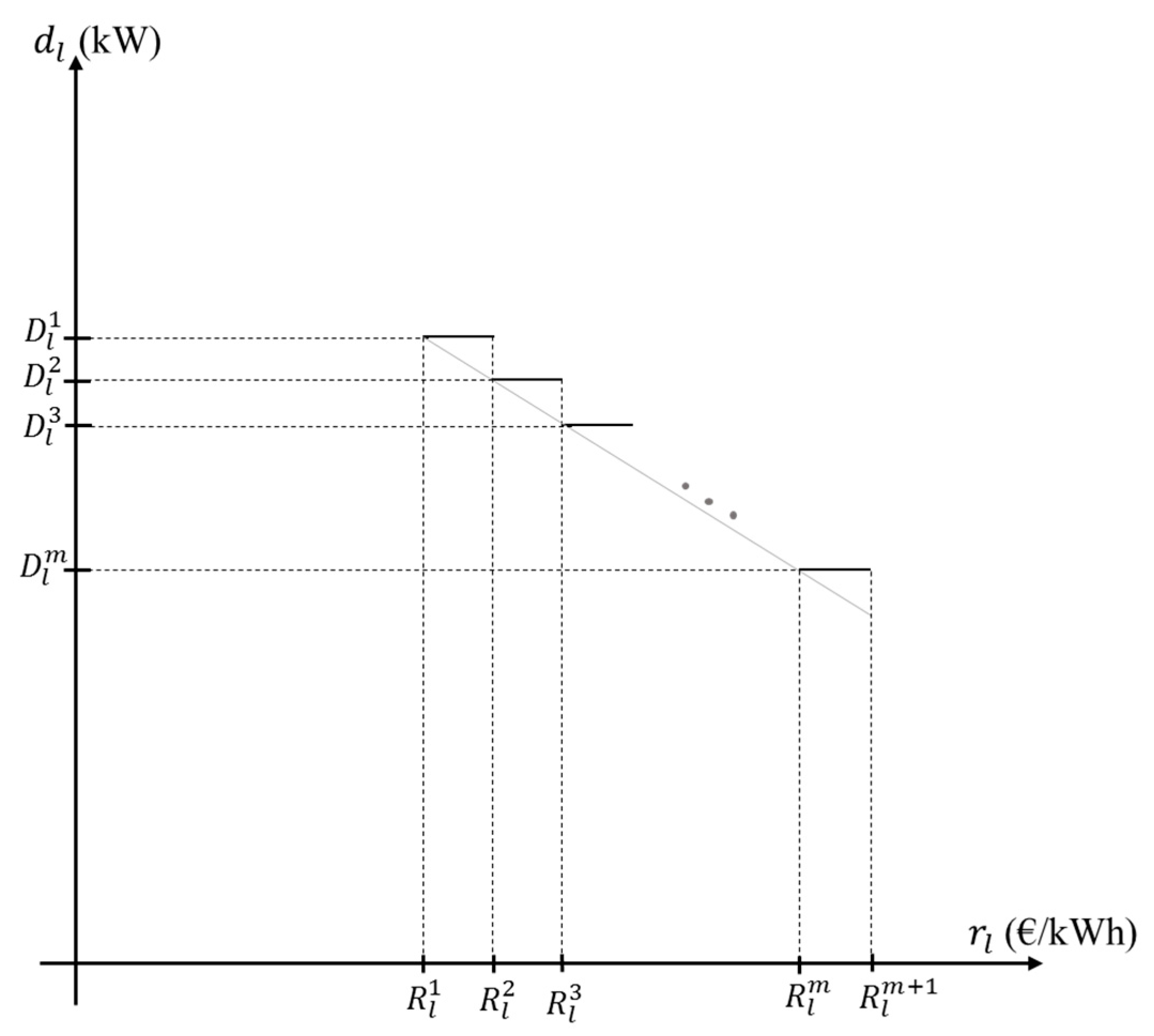
In this model, the schedules are dependent on the customers’ baseline consumption. The demand baseline of each customer group can be obtained from the historical data. Using the linear demand function (1), replacing the demand with a linear function of the retail rates makes the revenue a nonlinear function of the demand. In order to make this term linear, the linear demand function is divided into
m linear segments.
Figure 3 shows the segments of the demand function. In this figure,
is a parameter denoting the expected consumption for each segment. Equation (3) expresses that the
in each time period is a linear function of
It is assumed that the retail rate
varies in this interval
.
is the length of each block. By increasing the number of segments and reducing the length of each block, the impact of this simplification will be reduced. The revenue function (1) is converted to (4), which is a mixed integer linear programming (MILP) term. Constraint (5) enforces the limit on the retail rate in each block.
is a binary decision variable, which is 1 when that segment is selected. Constraint (6) expresses that only one block is selected for each customer group at each time period.
The final retail rate and the respective expected demand are respectively calculated by Equations (7) and (8).
Using the above set of constraints, the revenue can be maximized from the customers’ leads by selecting high retail rates, especially when the customers are not so elastic. Therefore, it is essential to consider constraints that limit this effect. In this model, it is assumed that that the dynamic pricing can only shift the consumption without reducing the total energy consumption [
18]. The total consumption of controllable price elastic loads remains the same by using Constraint (9).
The main source for procuring the energy requirements of the customers is purchasing on the pool market. The total cost of procuring energy needs from the market is illustrated by Equation (10). At each node n, the REP buys
(kWh) at market price
(€/kWh). The variable
is the energy needs of each customer group, which will be purchased from the market. Equation (11) shows that the total purchase from the market at each node is equal to the summation of purchases for each customer group.
denotes the set of customers that are located at the same node. This node can refer to a specific distribution network. Generally, the locational marginal prices (LMPs) are discriminated by the nodes.
2.1. Forward Contracts
Prior to participating in the day-ahead market, the REP can make a bilateral agreement with the generation-side [
13]. This forward contracting is a complement for trading with an exchange or a pool market. It is a contract of buying and selling a specific amount of energy in the future at an agreed price. Retailing companies and generation companies both use this approach to hedge the price risk [
19]. These bilateral arrangements can be made between the REPs and the DG owners. The daily cost of procuring energy through bilateral trading is calculated with Equation (12), where
is procurement of power through bilateral agreement
f. This variable can vary in each time period, but it should be within the range determined by the generation company with which the REP is making the Contract (13).
is a binary variable, which is 1 if the bilateral agreement
f is selected. When a bilateral contract is selected, the retailer should procure part of its demand through this bilateral contract during all the periods in which the contract is offered.
Bilateral contracts in electricity markets can have different clauses, which are determined through negotiation between the two sides. These clauses cover specific circumstances such as when the DG unit cannot procure the agreed power or when the REP cannot consume the agreed energy. One of the conditions that is usually included in the contracts is compensating the difference between the actual pool price and the price of bilateral contracts. In this model, it is assumed that the difference is equally split between the two sides [
8]. Therefore, an additional term should be added to the cost function of Equation (14) [
8]. The REPs will earn when the pool price is below the price of the bilateral agreement.
Therefore, the cost of purchasing power through bilateral contracts is represented with Equation (15).
2.2. Call Options
REPs can also use call option contracts to protect themselves against the risks of market price spikes. A call option gives the REP the right to purchase a specific amount of electricity at a determined strike price before reaching the expiration time [
7,
20]. REPs should pay a fee called a premium for the right of buying power through call options [
7]. They exercise the options and pay the option price for power during the periods that the spot market prices are expected to spike. The cost of procuring energy through call options is shown in Equation (16), where the
is the power blocks of call option
j,
is the premium, and
is the price of call option
j. The binary variable
is 1 when the level
b is selected for call option
j, and
is 1 if the call option
j is exercised in time period
t.
The product of the two binary variables (i.e.,
and
) makes the call option cost a nonlinear term. Therefore, the auxiliary binary variable
is used in Equation (17) to make the call option cost linear with Constraints (18)–(20). Constraint (21) enforces that only one block should be selected.
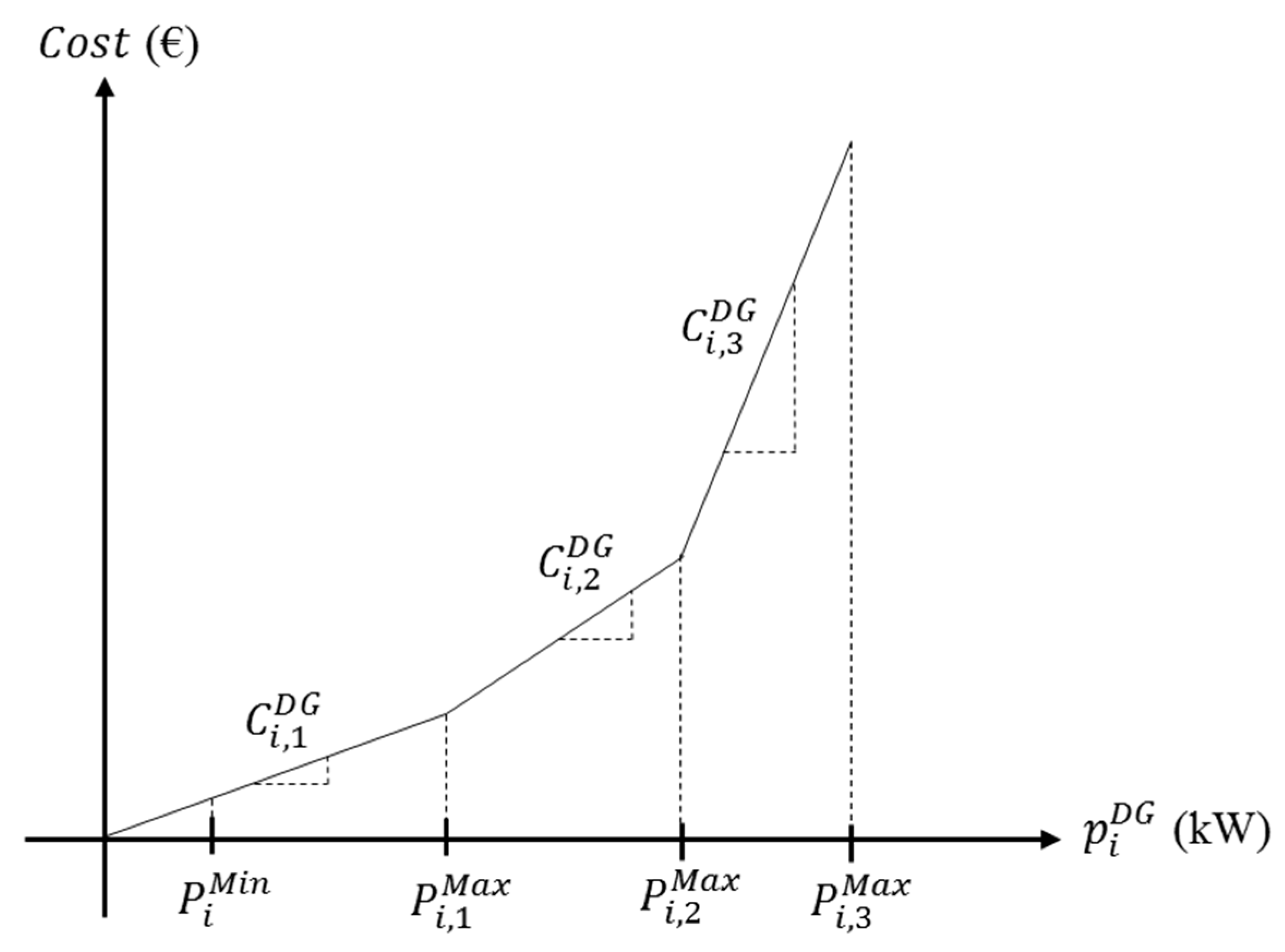
2.3. DGs
The linear cost function introduced in [
2] is used in this paper to model the operation cost of controllable DG units owned by the REP. The total generation cost of the self-generation DG units is represented with Equation (22). The total power generation of a DG unit
i in each time period (
) is the summation of the generation in all blocks (23). The relationship between the total cost and the generation of the DG unit
i is shown with a three-segment linear cost function in
Figure 4 [
2]. In each block, the generation cost is the slope of the segment in that block.
Constraints (24) and (25) force the DG production for each segment to be within the range. Segmentation is used to incorporate different generation costs. The generation cost of the DG increases as the production of the unit increases. The binary decision variable
is used to consider the commitment status of the DG units in each period.
Constraints (26) and (27) enforce the ramping up/down rate limits to the operation of DG units [
2]. The duration of each period (
τ), which is a fraction of 1 h, is incorporated in the right-hand side of Constraints (26) and (27) to limit the power increase/decrease when the time periods are less than or higher than one hour.
The consumption and energy procurement balancing constraint at each node is shown in Constraint (28).
3. Robust Optimization Model
Most of the methods used in the literature to tackle uncertainty in optimization problems require access to some historical data of the uncertain input. For instance, a probability density function is needed in probabilistic methods, and membership functions of the uncertain variables are required in the possibilistic approaches. The above methods cannot be used when the asset-light REP is subject to severe market price uncertainty and prediction is difficult or when estimating the probability distribution of the forecast error is impossible [
13]. Robust optimization has emerged as an efficient optimization technique, which reduces the sensitivity of the optimal solution to the changes in the input values [
13]. The robust optimization model is used when there is lack of data on the nature of the uncertainty. By solving a robust optimization model, the REP is assured that, though there might be an error in the price forecast, it is highly probable that the expected payoff will remain optimal [
4]. The robust optimization approach developed by [
21] is used in this paper. It offers the decision-maker in our problem the capability to control the tradeoff between payoff and robustness by varying a single parameter Γ. A maximization MILP problem can be represented in the following form:
The coefficients of the variable
are known in the MILP problem. Uncertainty can be attached to the set of the coefficients of the variable
x by modeling an uncertainty set
, where
. The predicted value and the maximum possible deviation are respectively shown with
and
. In other words, each coefficient
takes values in the interval
[
4,
5,
21]. The robust problem associated with Optimization Problems (29)–(32) can be represented in the following form:
An integer control parameter
is defined to control the level of robustness in the objective function. It takes values in
, where
. The influence of the cost deviations in the objective function can be tuned by changing the value of
. When it is at the minimum value, the influence of the deviations is ignored, and when it takes its’ maximum amount, all deviations are considered [
5]. The latter case leads to a comparatively more conservative solution. In Optimization Problems (33)–(39),
and
are the dual variables of MILP Problems (29)–(32).
is an the auxiliary variable used to make the problem linear.
The proposed MILP optimization model for the REP is rewritten here as a robust MILP. It is assumed that the market price is considered in the following range: . The uncertainty modeling of electricity prices is carried out within a linear structure, which does not add complexity to the model developed in the previous section.
The robust model of the REPs’ decision-making framework is represented in Equations (40)–(46).
4. Case Studies
The proposed decision-making framework is implemented in a General Algebraic Modeling System (GAMS) [
22] environment and solved by CPLEX solver [
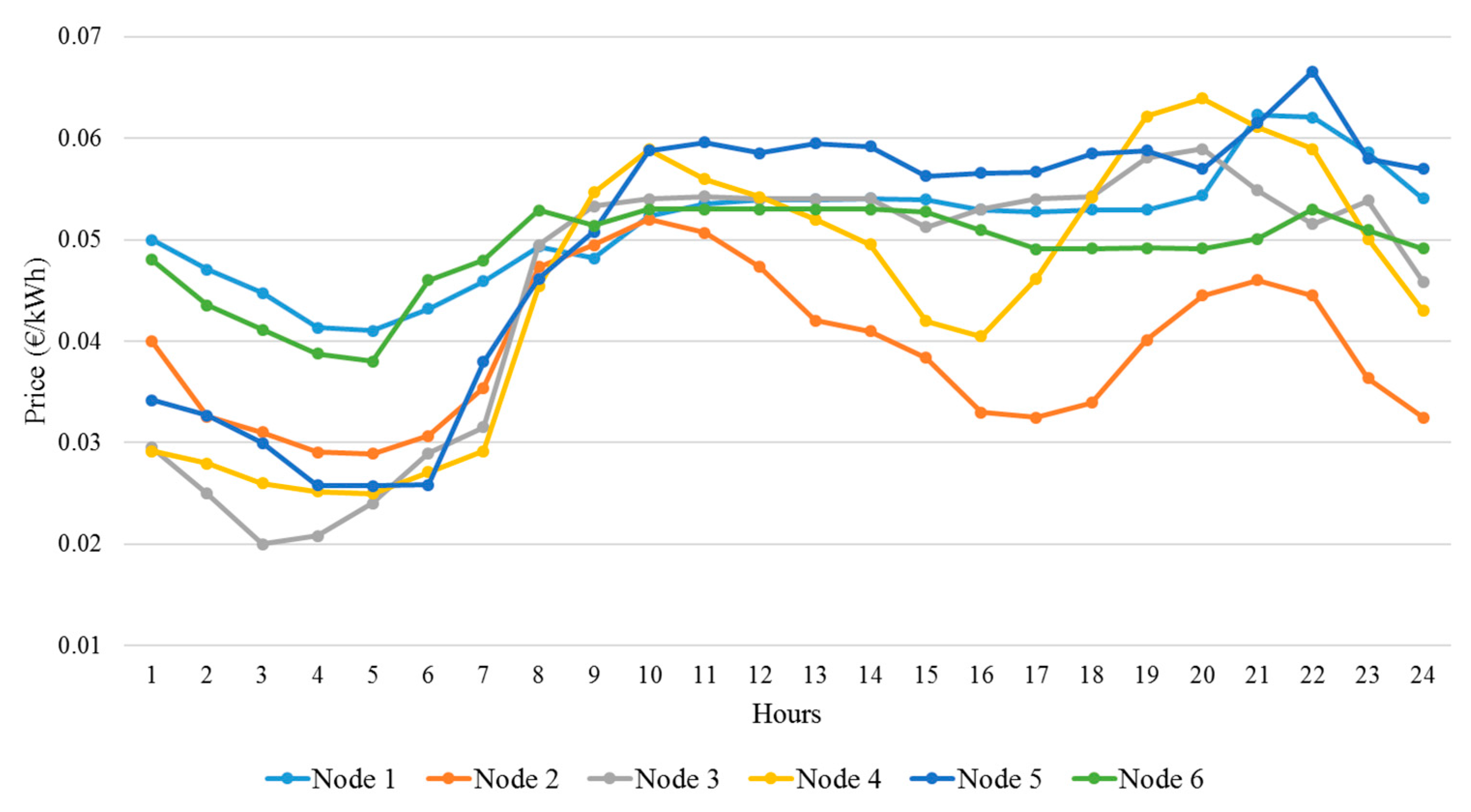
23]. It is applied for a REP with 10,679 residential customers divided into 14 customer groups. Each customer group contains electricity consumers with quite similar price elasticities of demand located at a similar node. The REP serves the loads at six different nodes. The number of residential consumers for each customer group and the nodes to which they are connected are shown in
Table 1. The values of forecasted nodal prices for all the nodes that the REP is serving are shown in
Figure 5. These values can be calculated with price forecasting techniques [
24,
25,
26,
27]. In this study the day-ahead market data published in PJM Energy Market [
28] is modified and used to represent the forecasted market data.
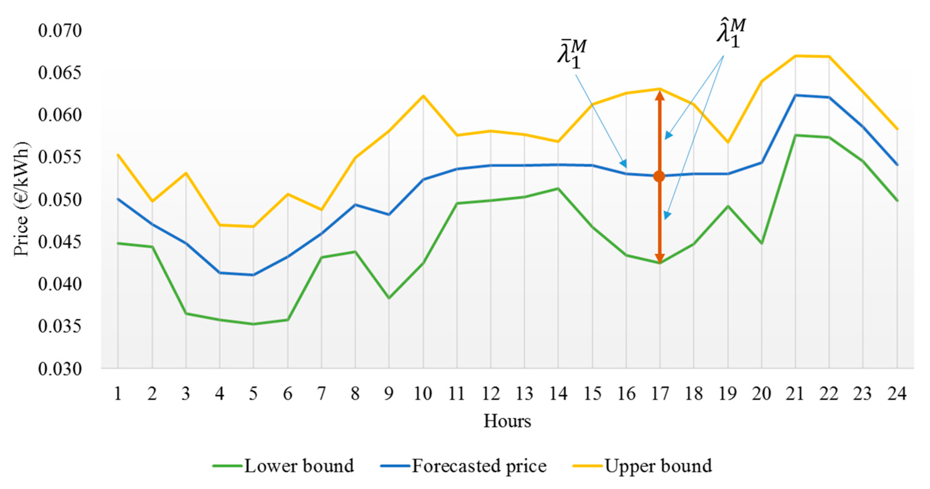
The forecasted market price and the price confidence interval for node 1 are depicted in
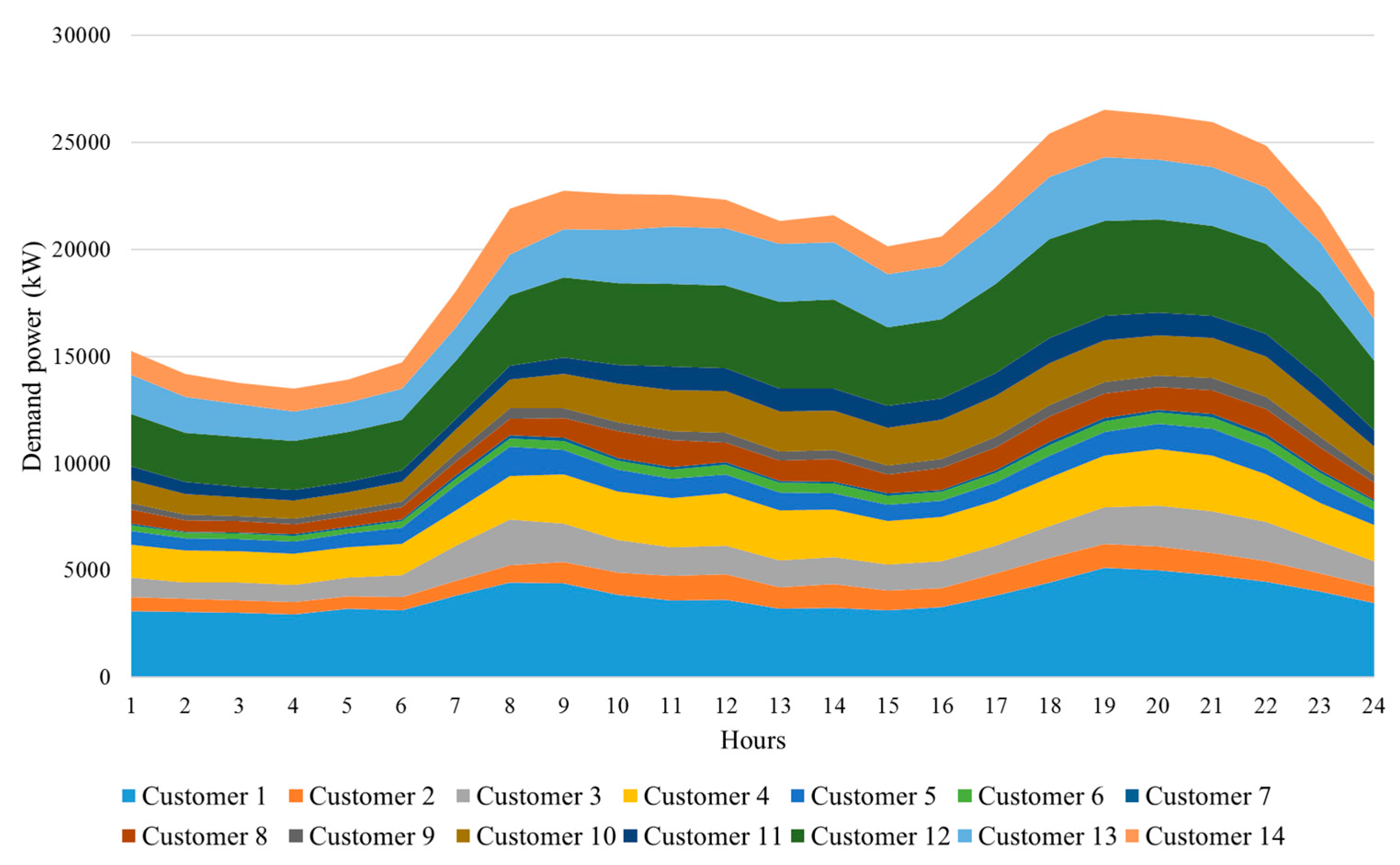
Figure 6 as an example. For all nodes, similar confidence intervals are considered for the market price. It is assumed that the actual market price is in this interval. The forecasted demand of each customer group is shown in
Figure 7. Actual consumption data is used in this study to represent the forecasted demands. The data is collected from a dataset gathered by Imperial College, Électricité de France (EDF), and UK Power Networks as part of the Low Carbon London project [
29] and from the dataset provided by Northwest Energy Efficiency Alliance (NEEA) [
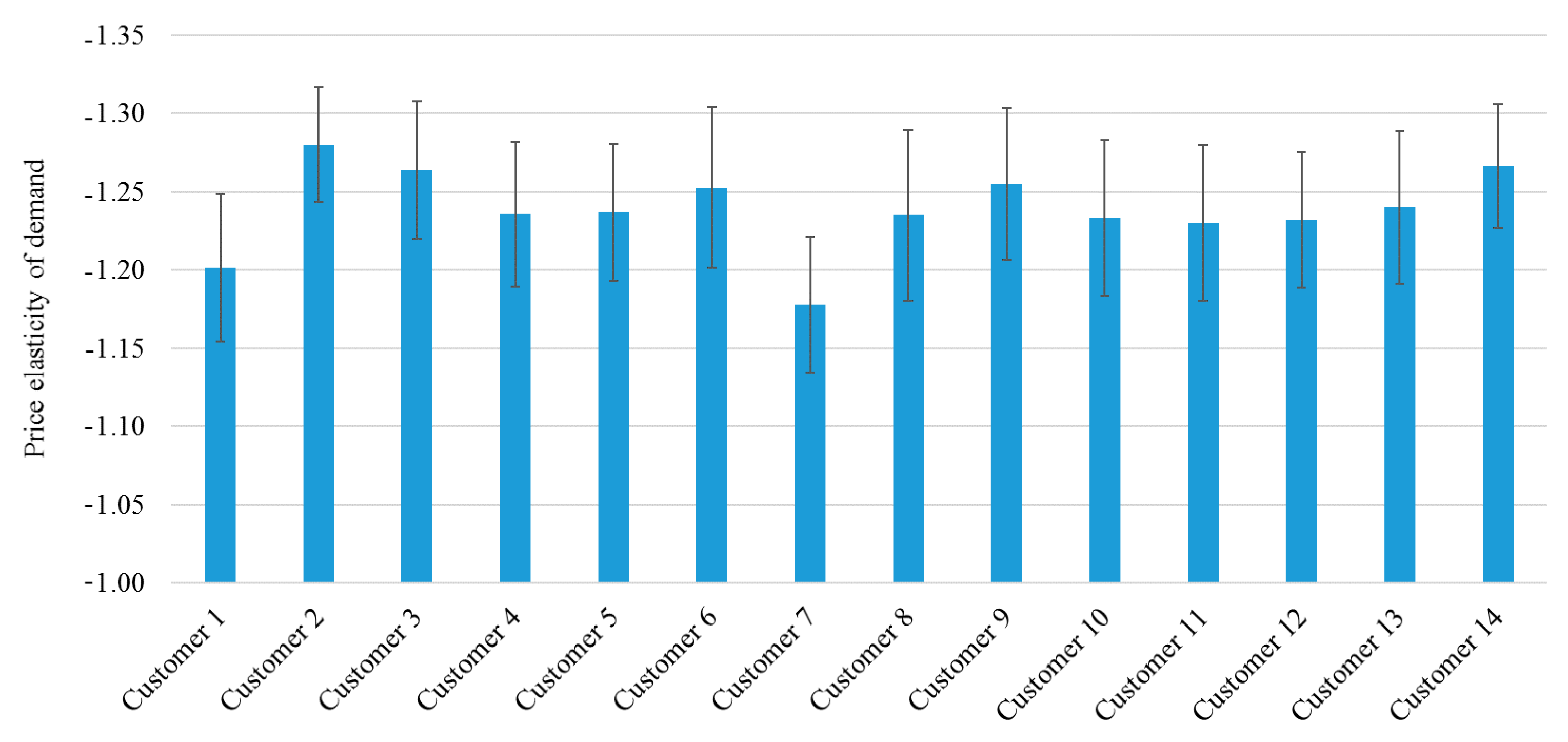
30]. The consumption of the residential customers is considered flexible and responsive to the changes of retail rates. The average of the hourly price elasticity of the demand of each customer group is shown in
Figure 8. The REP considers different demand functions for each customer group during each period. These demand functions are calculated based on the historical data. According to this historical information, a specific range is considered, and it is assumed that the demand changes in this range. In order to keep the problem linear, 100 segments are defined for the demand function in this range. The length of each block is small enough so that it does not significantly influence the results and also maintains the price elasticity of demand. For instance, the length of the blocks for customer group 1 at time period 1 is
, and the difference between the load demand in two consecutive segments is 0.0078 kW.
The REP uses different tools such as forward contracts, self-generation DG units, and call options to procure part of the energy requirements of their customers.
Table 2 shows the characteristics of the forward contracts. It is assumed that the REP can benefit from eight different forward contracts. The nodes that these contracts offer and the periods for which they are available are shown in
Table 3. In
Table 3, the characteristics of the DG units are shown. In the linear model for the DG cost, different segments were considered for the generation cost. The limits of five blocks and the generation cost of each block are given in the table. The ramping up and ramping down of the DG units are also shown in the table. The call options, their respective nodes, and the available periods are shown in
Table 4.
The proposed model has the potential to schedule for different time resolutions. Since some options that the REPs should make are defined at hourly levels [
7], hourly resolution is used in this model. In order to evaluate the proposed decision-making model, the initial problem and its robust counterpart are solved for the following cases:
Case 1: call options, forward contracts, and DG units as risk hedging tools.
Case 2: call options and forward contracts as risk hedging tools.
Case 3: call options and DG units as risk hedging tools.
Case 4: forward contracts and DG units as risk hedging tools.
The optimal percentages of using each possible tool in procuring the energy requirements of the consumers at each node are represented in
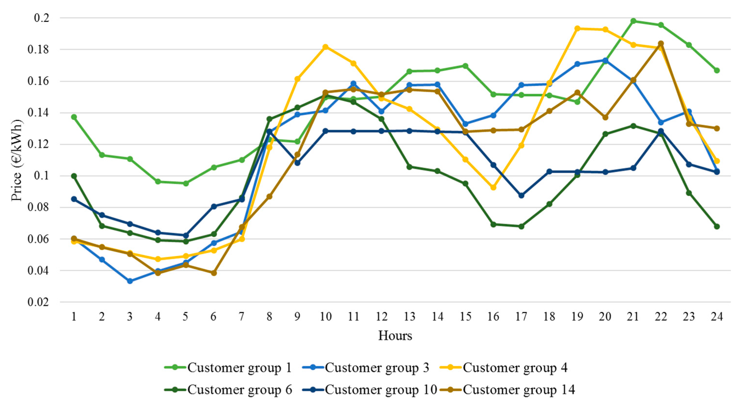
Table 5 for the case studies. Each case study has been solved as a deterministic problem and a robust model. The market in all cases is the primary source for serving the energy needs of the residential consumers. Depending on the case and the node, the percentages at which other sources such as DG units, forward contracts, and call options are used changes. The main decision variables in this decision-making framework are the time-variable retail rates that the REP calculates in the optimization problem. The optimal retail rates, which guarantee maximum payoff for the REP, are depicted in
Figure 9 for six selected customer groups. One customer group from each node is selected in this figure.
The differences between the total payoffs of the REPs in each case are shown in
Table 6. As the main source of procuring energy requirements is the market, the differences between the cases are negligible. It is also obvious that, in the deterministic model, in which the REP considers the average expected market price to calculate the time-variable retail rates, higher profits are achieved in the optimization problem. The REP uses the robust formulation to hedge against the risks associated with price uncertainty. Therefore, the expected payoff of the REP will be lower in this case. The difference is paid to protect their commercial decisions against market price volatility. It is assumed that the REP is making the most conservative decision in the robust model (Γ = 24). The interesting finding in this table is the difference between the two robust models: one with dynamic rates and one with fixed rates. The average value of the optimal dynamic rates is used for the fixed rate. The results reveal that the REP can save an average amount of 2224 Euros per day by offering dynamic rates to its customers. In the robust model with fixed rates, the same decisions that the REP made in the case with dynamic rates are considered. It shows that offering time-variable rates to retail customers can provide higher payoffs for the REPs.
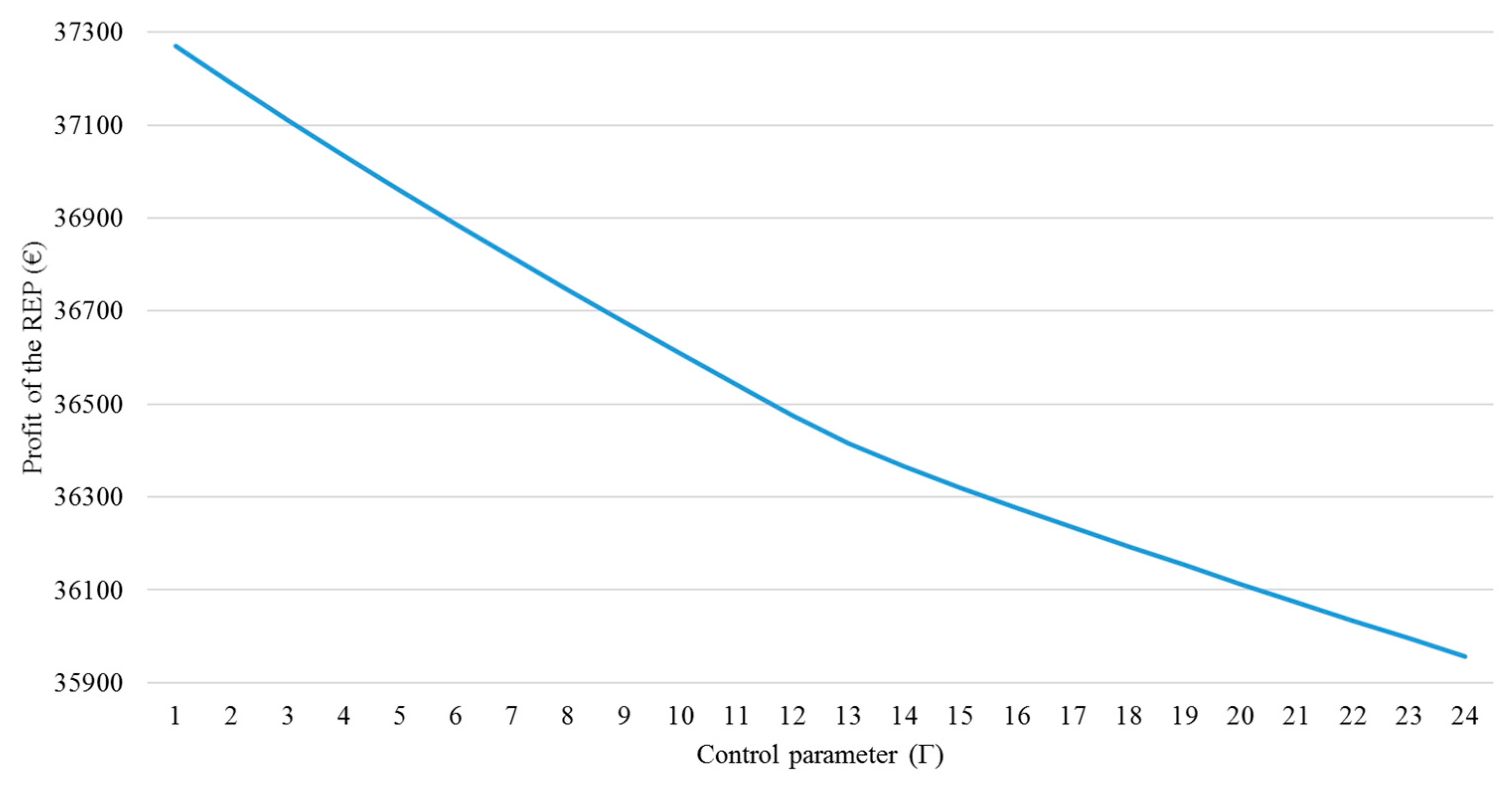
The REP should manage financial risks by determining an optimal value for the control parameter
.
Figure 10 shows the profit of the REP versus the changes of the control parameter for Case 1. In order to achieve this graph, Optimization Problems (40)–(46) are solved for different integer values of the control parameter. The REP can select a situation between risk neutrality on the left of this graph and risk aversion on the right. The level of robustness improves when the REP increases the value of the control parameter. The interesting finding here is that the optimal value of the REP’s profit is influenced only to a limited extent when the protection level increases. The payoff is penalized for 3.91% (i.e., 1406.47 Euros) when all the market price uncertainties are covered.
The main advantage of employing the robust optimization approach for REPs in comparison to the deterministic approach is ensuring higher payoffs when the worst scenario occurs. In this case, the worst scenario occurs when the wholesale market prices are at the highest bound. The payoff of the REP in the worst-case market price realization is shown
Table 7. The decisions that the REP makes with the deterministic approach lead to lower payoffs compared with the robust approach when the worst-case market price realization occurs.


