Article

An Ensemble Model Based on Machine Learning Methods and Data Preprocessing for Short-Term Electric Load Forecasting

1
School of Economics and Management, China University of Geosciences, Wuhan 430074, China
2
Mineral Resource Strategy and Policy Research Center, China University of Geosciences, Wuhan 430074, China
*
Author to whom correspondence should be addressed.
Energies 2017, 10(8), 1186; https://doi.org/10.3390/en10081186
Submission received: 14 July 2017 / Revised: 4 August 2017 / Accepted: 7 August 2017 / Published: 11 August 2017
(This article belongs to the Section F: Electrical Engineering)

Abstract

:
The experience with deregulated electricity market has shown the increasingly important role of short-term electric load forecasting in the energy producing and scheduling. However, because of nonlinear, stochastic and nonstable characteristics associated with the electric load series, it is extremely difficult to precisely forecast the electric load. This paper aims to establish a novel ensemble model based on variational mode decomposition (VMD) and extreme learning machine (ELM) optimized by differential evolution (DE) algorithm for multi-step ahead electric load forecasting. The proposed model is novel in the sense that VMD is firstly applied to decompose the original electric load series into a set of components with different frequencies in order to effectively eliminate the stochastic fluctuation characteristic so as to improve the overall prediction accuracy. The proposed ensemble model is tested using two electric load series collected from New South Wales (NSW) and Queensland (QLD) in the Australian electricity market. The experimental results show that: (1) the data preprocessing by VMD can effectively decrease the stochastic fluctuation characteristics that existed in the electric load series, consequently improving the whole forecasting accuracy, and; (2) the proposed forecasting model performs better than all other benchmark models for both one-step and multi-step ahead electric load forecasting.

1. Introduction

Electric power is a clean and efficient energy which plays an increasingly vital role in our daily life. Compared with traditional energy such as natural gas, coal and oil, electric power is more suitable and efficient for the requirement of environment-friendly society. In the field of power system planning, the accuracy of electric load forecasting is of great importance for energy generating capacity scheduling and power system management [1,2]. An overestimation may waste many energy resources and significantly improve the operational costs, and an underestimation will decrease the reliability of the power system and cannot meet the requirement of electricity utilization [3]. Therefore, accurate electric load forecasting is essential and significant for power systems. However, because the electric load series is affected by many complicated influencing factors, it is really a challenging job to accurately predict the electric load.
Over the past several decades, various interesting models for the electric load forecasting have been established, and they can be generally divided into the following two types. The first type is the multi-factor forecasting method, which needs to search the causal relationships between different influencing factors and forecasting values [4]. The other one is time series forecasting method which is based on the historical series. As is mentioned above, the electric load series is affected by various complicated and nonobjective factors which are very difficult to be controlled in practical application and, consequently, it is a very challenging job to establish an accurate forecasting model by utilizing the multi-factor forecasting method. Based on the above considerations, lots of researchers turn to utilizing the time series forecasting method to forecast electric load [5]. Compared to multi-factor forecasting method, the time series forecasting method is much easier and quicker. The most frequently and widely used time series forecasting models can be further divided into the following three subcategories: statistical models; machine learning models, and; hybrid models [6]. As for the statistical models, the auto-regressive moving average (ARMA), auto-regressive integrated moving average (ARIMA), generalized autoregressive conditional heteroskedasticity (GARCH), vector auto-regression (VAR), and Kalman filters methods are widely used in the electric load forecasting areas. For example, Pappas et al. [7] established an ARMA model for short-term electric load forecasting, and the results showed the good performance of the proposed model. Kavousi-Fard and Kavousi-Fard [8] proposed a new hybrid model based on ARIMA for short-term load forecasting. Takiyar et al. [9] developed a GARCH-based hybrid model for short-term electric load forecasting. Garcia-Ascanio and Mate [10] utilized VAR-based interval time series model to forecast electric load forecasting. Takeda et al. [11] developed an ensemble model based on Kalman filter for short-term electric load forecasting, and the experiment indicated that the predicting accuracy of the proposed model is obviously better than that of the present state-of-the-art models.
With the fast development of machine learning method, many of them have been widely used in various forecasting issues, such as artificial neural network (ANN), extreme learning machine (ELM) and support vector machine (SVM). Yolcu et al. [12] developed a new ANN model based on both linear and nonlinear structures for time series predicting. Gutierrez-Corea et al. [13] focused on the usage of ANN in short-term global solar irradiance forecasting. Li et al. [14] proposed a novel model based on modified artificial bee colony (MABC) and ELM for short-term electric load forecasting, and the experimental results showed that the proposed hybrid model owned the best forecasting ability with comparison to the other benchmark models adopted in their paper. Zhou et al. [15] developed a hybrid model based on SVM for short-term wind speed forecasting. Chen and Lee [16] established a weighted least square support vector machine (LSSVM) model based on learning system for time series forecasting, and the experimental results demonstrated the effectiveness of the proposed model.
By integrating the advantages of different single forecasting models, hybrid forecasting models generally performs better than the single forecasting models and therefore are widely used in many forecasting areas. For example, Liu and Shi [17] proposed an ARMA-GARCH model for predicting short-term electricity prices. Voyant et al. [18] developed an original technique to forecast global radiation based on a hybrid ARMA-ANN model for numerical weather forecasting. Ismail et al. [19] developed a hybrid self-organizing maps (SOM)-LSSVM model combining SOM and LSSVM for time-series predicting, and the experiment in the paper showed that SOM-LSSVM outperforms the single LSSVM model. Even though the hybrid model performs better than the single forecasting model, they still cannot effectively deal with the nonlinear and nonstationary characteristics associated with majority of time series in practical life. Therefore, many researchers have integrated various data preprocessing techniques into the forecasting models in order to effectively decrease the forecasting errors. The most widely used data preprocessing techniques includes empirical mode decomposition (EMD), ensemble empirical mode decomposition (EEMD), wavelet packet transform (WPT) and variational mode decomposition (VMD). Liu [20] predicted short-term wind speed by a hybrid model combining wavelet transform (WT) and SVM optimized by genetic algorithm, and the simulation results demonstrated that the proposed hybrid model is more efficient than the other comparison models adopted in their paper. Wang et al. [21] developed a hybrid forecasting model based on WPT, particle swarm optimization (PSO), simulated annealing (SA), phase space reconstruction (PSR) and LSSVM for multi-step ahead wind speed forecasting, and the case studies showed that the proposed model outperformed all the other comparison models. Zhang et al. [22] investigated the usage of WT-LSSVM model in the time series forecasting of fair-weather atmospheric electric field, and the experimental results showed that the proposed WT-LSSVM model is a superior method compared to the single LSSVM and ANN model. Wang et al. [23] developed a two-layer decomposition model for multi-step ahead electricity price forecasting, where VMD is specifically applied to decompose the high frequency sub-signals generated by fast ensemble empirical mode decomposition (FEEMD), and the experimental results illustrated the superior performances of the proposed model. For more details on different forecasting models, the reader can refer to the references [24,25,26], among others.
Although VMD has been utilized in many forecasting issues such as forecasting of wind power [27] and financial time series [28], the advantages of VMD have not been confirmed in the electric load forecasting area. Based on the above considerations, this paper aims to establish an ensemble model combining VMD and an improved ELM for short-term electric load forecasting. The process of the proposed model can be summarized into the following three steps: first, VMD is used to decompose the original electric load series into a set of components with different frequencies in order to effectively decrease the stochastic fluctuation characteristics; then, each component is forecasted using the ELM model whose initial weights and thresholds between the input layer and hidden layer are optimized by DE algorithm; finally, the ultimate forecasting series of electric load is obtained by aggregating the forecasting value of each component. Two real-world electric load series collected from New South Wales (NSW) and Queensland (QLD) located in Australia are used to test the effectiveness of the proposed ensemble model.
Based on aforementioned researches, the main novelties and contributions of this paper can be summarized to the following four aspects: (1) VMD technique is firstly applied to preprocess the electric load series in order to improve the overall forecasting accuracy; (2) VMD technique is combined with machine learning methods to develop a novel ensemble model for short-term electric load forecasting; (3) DE algorithm is employed to optimize the initial weights and thresholds of ELM in order to improve its function approximation ability; (4) the effectiveness of the proposed model is also examined by comparing with the forecasting models combining different decomposition techniques such as EMD and WT.
The rest of this paper is organized as follows. Section 2 firstly describes in detail the fundamental methods used in the paper, and then develops the hybrid VMD-DE-ELM model. Section 3 provides the data source and preprocessing results. Section 4 is the empirical study where the performance evaluating criteria, parameter settings and experimental results are presented. Section 5 concludes the paper.

2. Methodology

2.1. Empirical Mode Decomposition

Empirical mode decomposition (EMD) which is firstly proposed by Huang [29] is widely used signal decomposition method. Compared with other decomposition methods such as Fourier transformation and wavelet analysis, EMD owns many better temporal and frequency resolutions [30]. Due to the advantages of EMD, it has been widely used as a data preprocessing technique in many forecasting issues. EMD can effectively decrease the nonlinear, nonstable and stochastic characteristics associated with the signal through decomposing the signal into a set of components, that is, intrinsic mode functions (IMFs) and residual component. Each IMF generated by EMD has to meet the following two conditions: (1) for all IMFs, the number of extrema and the number of passing through zero must be equal or differ at most by one; (2) at any point, the mean value of the envelopes must be zero. Based on the above explanations, a time series denoted by signal p ( t ) could be disassembled through the following three steps.
Step 1: Find out all local maxima and minima of a signal p ( t ) . Connect all maxima by a cubic spline line to generate the upper envelop, and connect all minima by another cubic spline line to generate the lower envelop. The mean value of the upper envelop and the lower envelop is defined as m , and the difference of p ( t ) and m is defined as h , which is illustrated in Equation (1).
h = p ( t ) m
Step 2: Consider h as a new signal p ( t ) , and repeat Step (1) for enough times until h satisfies the conditions of IMF. The criterion (2) is used to decide if h is an IMF.
D m = t = 0 T | h ( m 1 ) ( t ) h m ( t ) | 2 t = 0 T | h ( m 1 ) ( t ) | 2
where, if D m is smaller than the predetermined value which can take the values between 0.2 and 0.3, h m can be an IMF. The first IMF is named as c 1 , which is the highest frequency component. The other components can be expressed as the Equation (3).
r 1 = P ( t ) c 1
Step 3: Consider r 1 as the new signal P ( t ) , repeat the operations in Step (1) and Step (2) for times until r j is smaller than the predetermined threshold or r j is a monotone function. Thus, all the IMFs and the residue r can be obtained.

2.2. Variational Mode Decomposition

Variational mode decomposition (VMD), a new effective signal decomposition method proposed by Dragomiretskiy and Zosso [31] in 2014, has been frequently used in many practical applications. Many previous researches have shown the good ability of VMD in the signal denoising field against other decomposition methods such as EMD and WT. In the decomposition process of VMD, each mode μ k can be compressed around a center pulsation ω k . The procedure for obtaining each mode’s bandwidth includes the following three steps: (1) for each mode, calculate the associated analytic signal with the benefit of Hilbert transform to obtain a unilateral frequency spectrum; (2) mix with an exponential tuned to the respective estimated center frequency in order to shift the mode’s frequency spectrum to baseband; (3) estimate the bandwidth of each model through Gaussian smoothness of the demodulated signal. Then, the constrained variational problem can be illustrated as follows:
min μ k , ω k = { k t [ ( δ ( t ) + j π t ) μ k ( t ) ] e j ω k t 2 }
Subject to
k μ k = f
where f represents the signal, μ denotes its mode, ω means the frequency, δ is the Dirac distribution, t is time script, k is the total number of modes, and represents the convolution function.
Then, the solution to the constrained variational problem (see Equation (4)) is the saddle point of the following augmented Lagrangian (L) expression:
L ( μ k , ω k , λ ) = α k t [ δ ( t ) + j π t μ k ( t ) ] 2 2 + f μ k 2 2 + λ , f μ k
where λ and α represents the Lagrange multiplier and the balancing parameter of the data-fidelity constraint, respectively. Consequently, the solutions for u and ω can be obtained according to the following two formulas:
μ n n + 1 = ( f i k μ i + λ 2 ) 1 1 + 2 α ( ω ω k ) 2
ω n n + 1 = 0 ω | μ k ( ω ) | 2 d ω 0 | μ k ( ω ) | 2 d ω
where n represents the number of iterations.

2.3. The DE-ELM Model

2.3.1. Extreme Learning Machine

Extreme learning machine (ELM), which was first proposed by Huang [32], is a single-hidden layer feed-forward neural network. In the ELM model, the weights of hidden layer nodes are randomly selected, and the output weights of ELM are determined by a least-squares solution. In the following section, we will introduce the ELM model in detail.
Let D = { ( x i , t i ) , i = 1 , 2 , , N } be a set with N different samples, where x i = [ x i 1 , x i 2 , , x i n ] T R is the inputs of sample, and t i = [ t i 1 , t i 2 , , t i m ] T R is the outputs of the sample. The activation function of ELM is g ( x ) , the threshold value of the hidden layer is b i and the output of ELM can be calculated by the following formula:
y j = i = 1 l β i g i ( x j ) = i = 1 l β i g i ( w i x j + b i ) j = 1 , 2 , , n
where w i = [ w i 1 , w i 2 , , w i n ] is the weights between the input layer and the hidden layer and β i = [ β i 1 , β i 2 , , β i m ] is the weights between the hidden layer and the output layer.
Formula (9) can also be denoted as Y = H β , where Y represents the output of ELM and H means the output matrix of the hidden layer. The output matrix H can be formulated as follows:
H ( w 1 , , w l ; b 1 , , b l , x 1 , , x n ) = [ g ( w 1 x 1 + b 1 ) g ( w 2 x 1 + b 2 ) g ( w l x 1 + b l ) g ( w 1 x 2 + b 1 ) g ( w 2 x 2 + b 2 ) g ( w l x 2 + b l ) g ( w 1 x n + b 1 ) g ( w 2 x n + b 2 ) g ( w l x k + b l ) ] n × l

2.3.2. Differential Evolution Algorithm

Differential Evolution (DE) algorithm, a simple population-based stochastic evolutionary algorithm first developed by Storn and Price [33], has been utilized for solving the combinatorial optimization problems in many application areas. Compared to other optimization algorithms, DE algorithm is easier and quicker, and only requires few control parameters. Generally, DE algorithm contains the following four steps: (1) initialization; (2) mutation; (3) crossover, and; (4) selection. The detailed information for each step is provided as follows:
Step 1: Initialize the population. The population of DE algorithm is initialized using the following formula.
x j , i , o = x j , min + r a n d i , j ( 0 , 1 ) × ( x j , max x j , min )
where x j , i , o represents the value of ith individual in the 0th generation and jth dimension.
Step 2: Mutation. Randomly select the following three indices, m , i and j , m i j , then, a mutant vector V k , G can be obtained according to the following formula.
V k , G = X m , G + F ( X i , G X j , G )
where k m i j , F represents a scaling factor and F [ 0 , 1 ] , X m , G denotes the base vector.
Step 3: Crossover. The purpose of crossover operation is to increase the multiplicity of the perturbed parameter vectors. The trial point U j , k , G + 1 is established from its parents V j , k , G + 1 and X j , k , G by the following formula.
U j , k , G + 1 = { V j , k , G + 1    if ( r a n d b ( j ) C R )   or   j = r n b r ( i ) X j , k , G     if ( r a n d b ( j ) > C R   and   j r n b r ( i ) )    j = 1 , , D ,
where C R is crossover probability and C R [ 0 , 1 ] , r n b r ( i ) is a randomly selected index in the set of { 1 , 2 , 3 , , D } , which ensures that U j , k , G + 1 obtains at least one parameter from V j , k , G + 1 . The trial vector is formed of both current parameter vectors and mutant vector parameters.
Step 4: Selection. The trial vector X i , G + 1 can be obtained by comparing the fitness value of the vector obtained through mutation and crossover, and the process can be denoted as follows:
X i , G + 1 = { U i , G    if f ( U i , G ) f ( X i , G ) X i , G    otherwise
Step 5: Repeat the above operations and stop the DE algorithm if the result satisfies the error requirement or the maximum number of iterations is reached. Otherwise, return to Step (2).

2.3.3. The DE-ELM Model

In order to reduce the non-stationarity and non-linearity characteristics of ELM forecasting model, DE algorithm is applied to optimize the initial weights and thresholds between input layer and hidden layer of ELM model. When the DE algorithm is stopped in the training process, the ELM model is established based on the optimized weights and thresholds determined by DE algorithm, and can be used to forecast the electric load series directly in the testing process.
F f i t n e s s = 1 N t = 1 N ( X ^ ( t ) X ( t ) ) 2
The fitness function of DE algorithm is the root mean square error (RMSE) of forecasting which is defined as follows:
Step 1: Initialize the individuals and the parameters of DE algorithm;
Step 2: Set the iterative variable and calculate the fitness value of each individual by using Equation (15). Stop the DE algorithm when the stop criterion is satisfied. Go to Step (4);
Step 3: Update the population. Go to Step (2);
Step 4: When DE algorithm is stopped, the optimal individual is taken as the initial connection weights and thresholds of ELM;
Step 5: Train and test ELM based on the training and testing samples.

2.4. The VMD-DE-ELM Forecasting Model

In this paper, an ensemble model based on machine learning methods and data preprocessing is proposed for short-term electric load forecasting. The basic structure of the ensemble method is based on decomposition and ensemble, which is shown in Figure 1 where Mode1′, Mode2′, ..., Moden′ respectively represent the forecasting values of Mode1, Mode2, ..., Moden.
The steps of the proposed ensemble model are shown as follows:
Step 1: Data preprocessing. VMD is used to decompose the original electric load series into several sub-series with different frequencies, namely, Mode 1 , Mode 2 , , Mode n ;
Step 2: Individual mode forecasting. Each mode is forecasted using the ELM model improved by the DE algorithm, and the forecasting result of each mode is obtained, namely, Mode 1 , Mode 2 , , Mode n ;
Step 3: Equal-weight aggregation. The modes generated by VMD are equally weighted and then aggregated in order to obtain the final forecasting results based on the following formula.
Final result = Mode 1 + Mode 2 + + Mode n

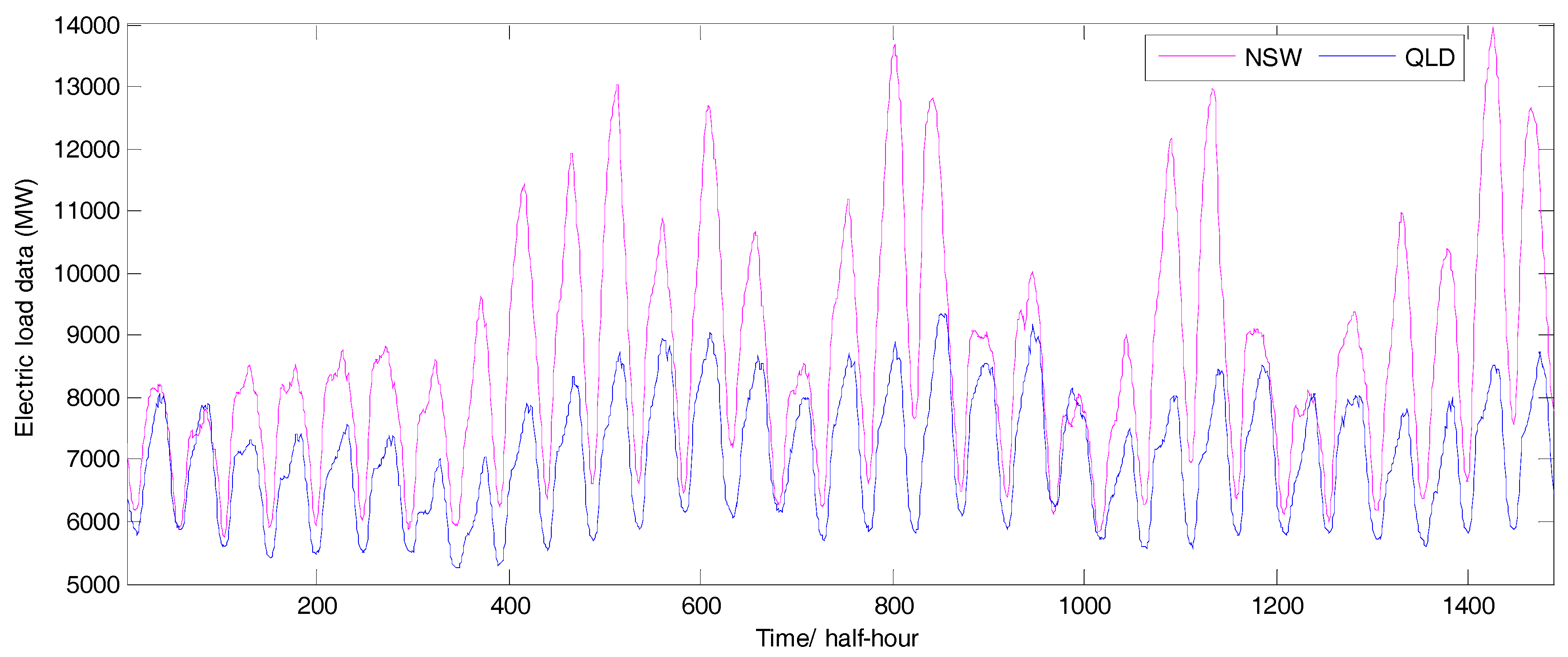
3. Data Description and Preprocessing

In this paper, two half-hour electric load series collected from NSW and QLD [34] are adopted to test the effectiveness of the proposed model. In Australia’s electricity market, there are 48 observation data points every day, which means the time gap of observation values is half an hour. In this paper, each electric load series contains 1488 observation data points (from 1 January 2017 to 31 January 2017), see Figure 2. Moreover, in each case, the 1st–1200th observation points are taken as training sets, and the rest, the 1201st–1488th observation points, are taken as testing sets. The descriptive statistics of the two electric load series is shown in Table 1.
As is shown in Table 1, the mean of electric load series of NSW is 8588.11, and the minimum value and maximum value of electric load series of NSW is 5767.31 and 13947.70, respectively. It is obvious that the maximum value of electric load series of NSW is larger than twice of the minimum value, which illustrates that the electric load series of NSW owns notable stochastic fluctuation characteristic. In QLD, the mean of electric load series is 7025.13, and the minimum value and maximum value of electric load series is respectively 5254.92 and 9357.09. The stochastic fluctuation characteristic of electric load series of QLD is also obvious. In addition, it should be noted that all numerical experiments in this paper are coded in MATLAB R2010a.
In order to make the forecasting results own more practical significance, this paper adopts multi-step ahead electric load forecasting. Compared with one-step ahead forecasting, multi-step ahead forecasting can supply more information for electricity market participants. Since multi-step ahead forecasting has to deal with many other additional complications such as the accumulation of errors, increased uncertainty and reduced accuracy [35], it is therefore more difficult to obtain precise forecasting results. This paper aims to propose an ensemble model for electric load forecasting over different horizons. Different horizons have different practical meanings. For instance, as for the half-hour data source, four-step ahead represents two-hour ahead, eight-step ahead represents four-hour ahead, and twelve-step ahead represents six-hour ahead. Furthermore, as shown in Figure 3, we take four-step ahead forecasting as an example to clearly interpret the multi-step ahead forecasting process. As shown in Figure 3, in the training process, the input and output datasets of DE-ELM model for four-step ahead forecasting are respectively { { x 1 , x 2 , , x 8 } , { x 2 , x 3 , , x 9 } , , { x 1189 , x 1190 , , x 1196 } } and { x 12 , x 13 , , x 1200 } , and in the testing process, the input and output datasets of DE-ELM model are respectively { { x 1190 , x 1191 , , x 1197 } , { x 1191 , x 1192 , , x 1198 } , , { x 1477 , x 1478 , , x 1484 } } and { x 1201 , x 1202 , , x 1488 } .

4. Empirical Study

4.1. Performance Criteria of Forecasting Accuracy

This paper selects the following three error measures to evaluate the performances of the proposed ensemble model: mean absolute error (MAE), root mean square error (RMSE) and mean absolute percentage error (MAPE). The computational formulas of these three error measures are provided as follows:
MAE = 1 N t = 1 N | X ^ ( t ) X ( t ) |
RMSE = 1 N t = 1 N ( X ^ ( t ) X ( t ) ) 2
MAPE = 1 N t = 1 N | X ^ ( t ) X ( t ) X ( t ) |
where N represents the number of observations, X ( t ) means the actual electric load value at time t , and X ^ ( t ) denotes the forecasting value at time t .

4.2. Multi-Step Ahead Electric Load Forecasting in NSW

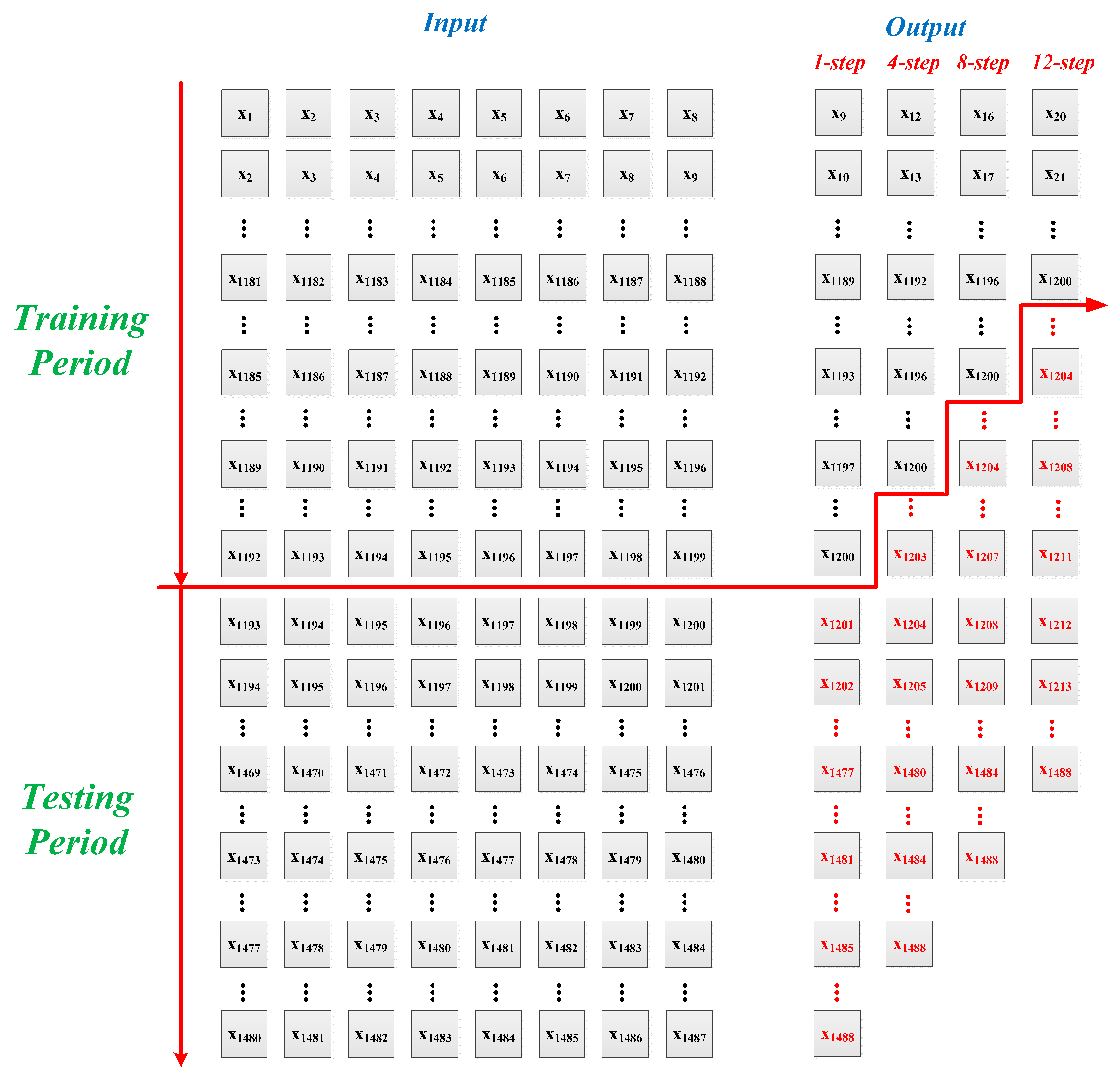
4.2.1. Data Preprocessing of the Original Electric Load Series

The electric load series is preprocessed using VMD in order to effectively decrease the stochastic fluctuations existing in the data series. Much previous research has shown that the number of components generated by VMD have significant effects on the characteristics of modes. In the decomposition process of VMD, more components will result in more stationary modes; however, more components might cause decomposition information loss and thus low forecasting accuracy. Based on the above considerations, after extensive numerical experiments, this study decomposes the data series into nine modes in order to ensure good forecasting accuracy. The decomposition results are shown in Figure 4 where the nine components are denoted by Mode1, Mode2, ..., Mode9, respectively.
Then, the forecasting issue turns to the forecasting of each mode using the ELM model improved by the DE algorithm. In this study, the inputs of DE-ELM model are determined using the rolling technique proposed in the reference [36], that is, every eight continuous electric load data points are employed to predict the ninth one, the detailed procedure is provided in Figure 3. The parameter settings of DE algorithm including iteration number ( G e n ), population size ( P o p ), mutation control parameter ( F ) and crossover probability ( C r ) are all listed as follows: G e n = 100 , P o p = 30 , F = 0.9 and C r = 0.5 . The above input determination method of ELM model and parameter settings are utilized in all of the models adopted in this paper to ensure fair and effective comparisons among different models.

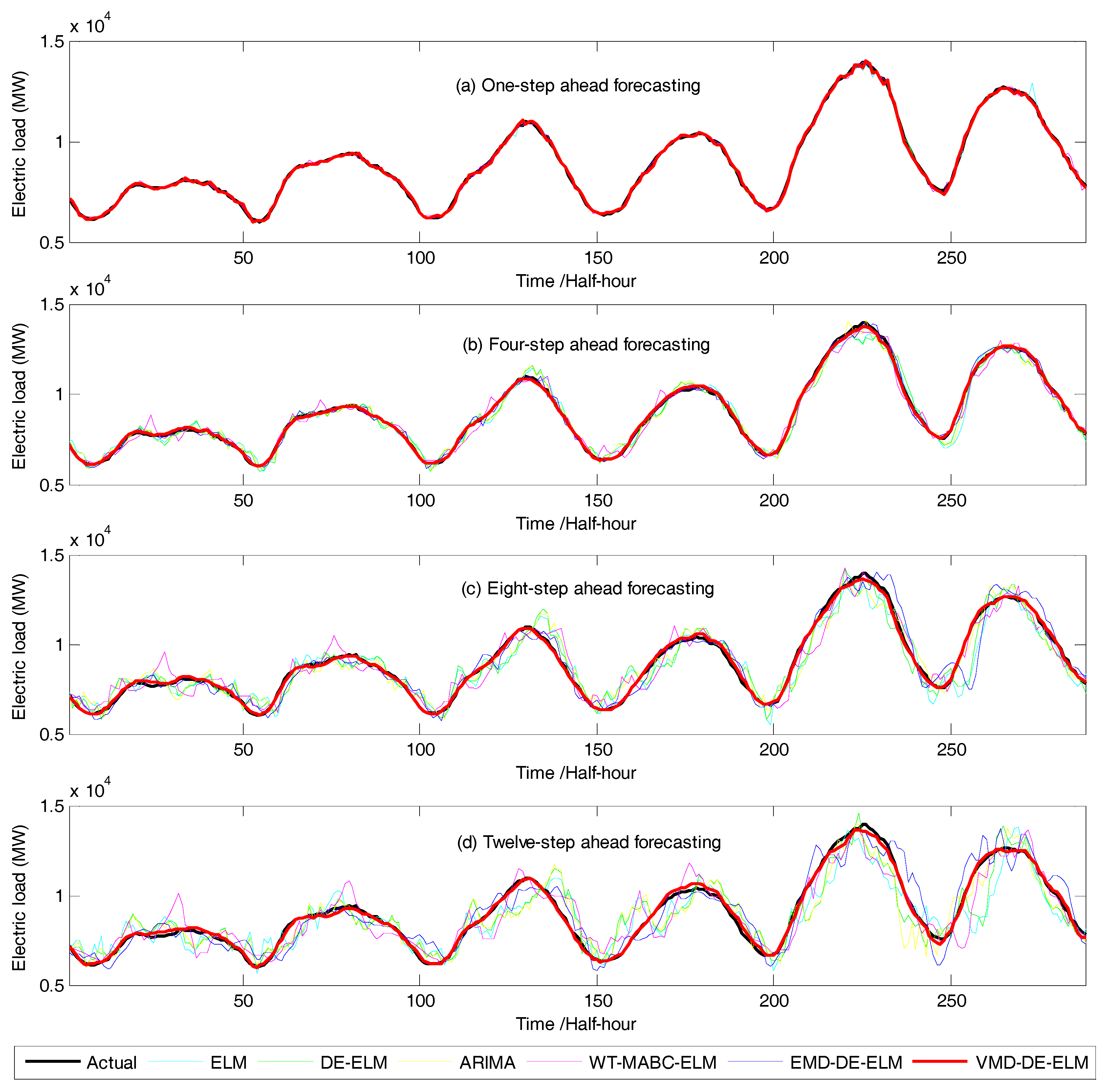
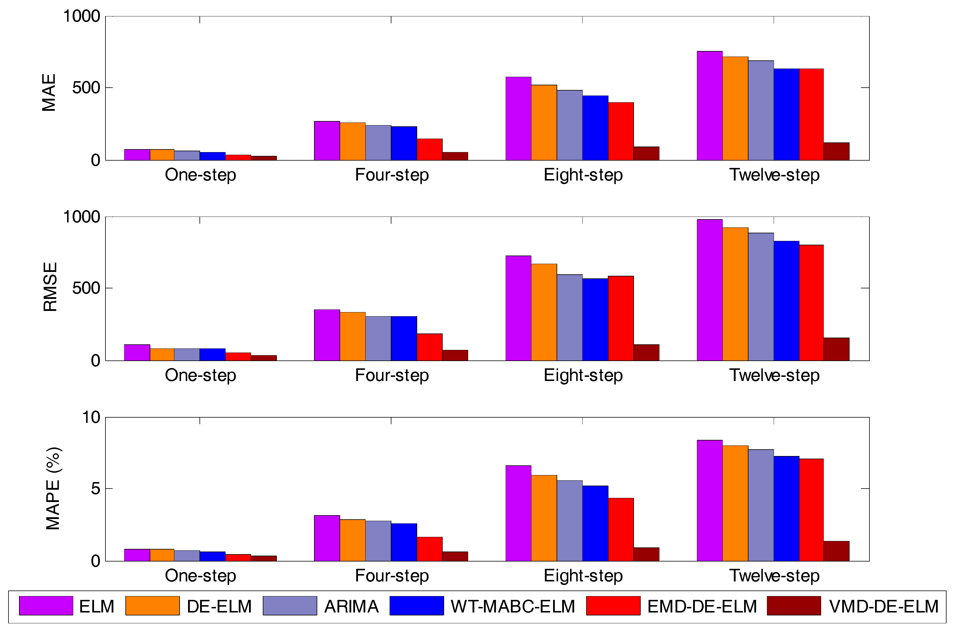
4.2.2. Forecasting Results, Comparative Analysis and Discussion

The effectiveness of the proposed forecasting is examined by comparing with the following two groups of benchmark models. The first group of models including ELM and DE-ELM models are adopted to confirm the influences of VMD and DE algorithm on the ELM model. The second group of models containing ARIMA, EMD-DE-ELM and WT-MABC-ELM models are selected to verify the reliability, practicability and portability of the developed model. The forecasting performances and the forecasting errors of all the above models are provided in Figure 5 and Table 2, respectively.
In order to show the comparison more clearly, three histograms based on the MAE, RMSE and MAPE values of all the considered models in the paper are also presented in Figure 6. As shown in Table 2 and Figure 6, the MAE, RMSE and MAPE values of the proposed model are all smaller than the other comparison models, which confirms the superior forecasting performance of the proposed model for both one-step and multi-step ahead electric load forecasting.
In order to well investigate why the proposed model performs better than other comparison models, this section conducts the following three comparative analysis: (1) VMD-DE-ELM and EMD-DE-ELM; (2) VMD-DE-ELM and DE-ELM; (3) ELM and DE-ELM. In order to more effectively compare the forecasting abilities of different models, the differences between the forecasting errors of different models are calculated according to the following formula: D F = ( e 2 e 1 ) / e 2 × 100 % , where D F is the error difference; e 1 and e 2 are the MAE, RMSE or MAPE value of the first and second models. The results of the three above comparative analysis are all shown in Table 3. Based on the results shown in Table 3, the following three findings can be derived: (1) the proposed model owns the better forecasting accuracy than EMD-DE-ELM, which confirms the good performance of VMD against EMD; (2) the forecasting errors of ELM is significantly decreased by combining the VMD, which illustrates that the data preprocessing by VMD can effectively decrease the stochastic fluctuation characteristics existed in the electric load series, and consequently improves the whole forecasting accuracy, and; (3) the forecasting ability of ELM model is effectively improved through integrating the DE algorithm, which is used to optimize the initial weight and thresholds, thus it can be concluded that the DE algorithm has positive influences on the performance of ELM model.

4.3. Multi-Step Ahead Electric Load Forecasting in QLD

In this section, the proposed model is tested using another real-world electric load series collected from QLD in order to verify its reliability and practicability. The forecasting results, including MAE, RMSE and MAPE values of all the models adopted in the paper, are provided in Table 4 and Table 5. Based on the results shown in Table 4 and Table 5, similar conclusions to that in the case of NSW are derived. It should be noted that because of different regional scales, population, geographical positions, climatic characteristics and industrial structures associated with NSW and QLD located in Australia, the two electric load series have significantly different complexities of irregularity, randomness and non-stationarity. In addition, the proposed VMD-DE-ELM model works only on the historical data series, consequently making different forecasting accuracies in the above two study cases. Nevertheless, all the experiment results in the two above cases can demonstrate the superiority of the proposed model.

5. Conclusions

In the deregulated electricity market, since the short-term electric load forecasting can provide lots of vital trading information for all of the market participants, thus it plays an increasingly important role for energy production, consumption and scheduling. However, various complicating influencing factors make the electric load series own severe stochastic fluctuation characteristics, which significantly increases the forecasting difficulties. This paper aims to establish an ensemble model based on VMD and ELM improved by the DE algorithm. In this proposed model, the electric load series is firstly preprocessed by VMD into a number of components in order to effectively decrease the stochastic fluctuation characteristics, and then each component is forecasted over different horizons using the optimized ELM model. Two real-world electric load series collected from NSW and QLD are used to test the proposed forecasting model, and comparative analysis based on two groups of benchmark models are conducted in this paper. Based on the experimental results, the following three conclusions can be derived: (1) the proposed forecasting model owns the better forecasting ability than all other comparison models, which illustrates the superior performances of the proposed model for both one-step and multi-step ahead electric load forecasting; (2) the forecasting errors of ELM are significantly decreased by combining the VMD, which illustrates that the data preprocessing by VMD can effectively decrease the stochastic fluctuation characteristics existing in the electric load series, and consequently improves the whole forecasting accuracy; (3) the forecasting ability of ELM model is effectively improved through integrating the DE algorithm, which is used to optimize the initial weight and thresholds, thus it can be concluded that the DE algorithm has positive influences on the performance of the ELM model.

Acknowledgments

This research was supported by the National Natural Science Foundation of China (Grant Nos. 71473232, 71573237); the Science Foundation of Mineral Resource Strategy and Policy Research Center, China University of Geosciences (Grant No. H2017011B).

Author Contributions

Yanbing Lin and Hongyuan Luo designed the experiments and collected the data. Deyun Wang conducted the case studies and analyzed the results. Haixiang Guo and Kejun Zhu provided critical review and manuscript editing. Yanbing Lin and Hongyuan Luo wrote the paper. All authors read and approved the final manuscript.

Conflicts of Interest

The authors declare no conflict of interest.

Abbreviations

VMDVariational mode decomposition
EMDEmpirical mode decomposition
EEMDEnsemble empirical mode decomposition
FEEMDFast ensemble empirical mode decomposition
IMFIntrinsic mode function
WPTWavelet packet transform
WTWavelet transform
ARMAAuto-regressive moving average
ARIMAAuto-regressive integrated moving average
GARCHGeneralized autoregressive conditional heteroskedasticity
VARVector auto-regression
ANNArtificial neural network
SVMSupport vector machine
LSSVMLeast square support vector machine
ELMExtreme learning machine
DEDifferential evolution
PSOParticle swarm optimization
SASimulated annealing
ABCArtificial bee colony
MABCModified artificial bee colony
SOMSelf-organizing maps
PSRPhase space reconstruction
RMSERoot mean square error
MAEMean absolute error
MAPEMean absolute percentage error
NSWNew south wales
QLDQueensland

References

  1. Abosedra, S.; Dah, A.; Ghosh, S. Electricity consumption and economic growth, the case of Lebanon. Appl. Energy 2009, 86, 429–432. [Google Scholar] [CrossRef]
  2. Adam, N.R.B.; Elahee, M.K.; Dauhoo, M.Z. Forecasting peak electricity demand in Mauritius using the non-homogeneous Gompertz diffusion process. Energy 2013, 36, 6763–6769. [Google Scholar] [CrossRef]
  3. Kavaklioglu, K.; Ceylan, H.; Ozturk, H.K.; Canyurt, O.E. Modeling and prediction of Turkey’s electricity consumption using Artificial Neural Networks. Energy Convers. Manag. 2009, 50, 2719–2727. [Google Scholar] [CrossRef]
  4. Chase, R.B.; Jacobs, F.R.; Aquilano, N.J. Operations Management for Competitive Advantage; McGraw-Hill/Irwin: New York, NY, USA, 2001. [Google Scholar]
  5. He, K.J.; Yu, L.A.; Tang, L. Electricity price forecasting with a BED (Bivariate EMD Denoising) methodology. Energy 2015, 91, 601–609. [Google Scholar] [CrossRef]
  6. Lei, M.; Luan, S.J.; Jiang, C.W.; Liu, H.L.; Zhang, Y. A review on the forecasting of wind speed and generated power. Renew. Sustain. Energy. Rev. 2009, 13, 915–920. [Google Scholar] [CrossRef]
  7. Pappas, S.S.; Ekonomou, L.; Karampelas, P.; Karamousantas, D.C.; Katsikas, S.K.; Chatzarakis, G.E.; Skafidas, P.D. Electricity demand load forecasting of the Hellenic power system using an ARMA model. Electr. Power Syst. Res. 2010, 80, 256–264. [Google Scholar] [CrossRef]
  8. Kavousi-Fard, A.; Kavousi-Fard, F. A new hybrid correction method for short-term load forecasting based on ARIMA, SVR and CSA. J. Exp. Theor. Artif. Intell. 2013, 25, 559–574. [Google Scholar] [CrossRef]
  9. Takiyar, S.; Upadhyay, K.G.; Singh, V. Fuzzy ARTMAP and GARCH-based hybrid model aided with wavelet transform for short-term electricity load forecasting. Energy Sci. Eng. 2016, 4, 14–22. [Google Scholar] [CrossRef]
  10. Garcia-Ascanio, C.; Mate, C. Electric power demand forecasting using interval time series: A comparison between VAR and iMLP. Energy Policy 2010, 38, 715–725. [Google Scholar] [CrossRef]
  11. Takeda, H.; Tamura, Y.; Sato, S. Using the ensemble Kalman filter for electricity load forecasting and analysis. Energy 2016, 104, 184–198. [Google Scholar] [CrossRef]
  12. Yolcu, U.; Egrioglu, E.; Aladag, C.H. A new linear and nonlinear artificial neural network model for time series forecasting. Decis. Support Syst. 2013, 54, 1340–1347. [Google Scholar] [CrossRef]
  13. Gutierrez-Corea, F.V.; Manso-Callejo, M.A.; Moreno-Regidor, M.P.; Manrique-Sancho, M.T. Forecasting short-term solar irradiance based on artificial neural networks and data from neighboring meteorological stations. Sol. Energy 2016, 134, 119–131. [Google Scholar] [CrossRef]
  14. Li, S.; Wang, P.; Goel, L. Short-term load forecasting by wavelet transform and evolutionary extreme learning machine. Electr. Power Syst. Res. 2015, 122, 96–103. [Google Scholar] [CrossRef]
  15. Zhou, J.Y.; Jing, S.; Gong, L. Fine tuning support vector machines for short-term wind speed forecasting. Energy Convers. Manag. 2011, 52, 1990–1998. [Google Scholar] [CrossRef]
  16. Chen, T.T.; Lee, S.J. A weighted LSSVM based learning system for time series forecasting. Inf. Sci. 2015, 299, 99–116. [Google Scholar] [CrossRef]
  17. Liu, H.; Shi, J. Applying ARMA-GARCH approaches to forecasting short-term electricity prices. Energy Econ. 2013, 37, 152–166. [Google Scholar] [CrossRef]
  18. Voyant, C.; Muselli, M.; Paoli, C.; Nivet, M. Numerical weather prediction (NWP) and hybrid ARMA/ANN model to predict global radiation. Energy 2012, 39, 341–355. [Google Scholar] [CrossRef]
  19. Ismail, S.; Shabri, A.; Samsudin, R. A hybrid model of self-organizing maps (SOM) and least square support vector machine (LSSVM) for time-series forecasting. Expert Syst. Appl. 2011, 38, 10574–10578. [Google Scholar] [CrossRef]
  20. Liu, D.; Niu, D.X.; Wang, H.; Fan, L.L. Short-term wind speed forecasting using wavelet transform and support vector machines optimized by genetic algorithm. Renew. Energy 2014, 62, 592–597. [Google Scholar] [CrossRef]
  21. Wang, J.Z.; Wang, Y.; Jiang, P. The study and application of a novel hybrid forecasting model—A case study of wind speed forecasting in China. Appl. Energy 2015, 143, 472–488. [Google Scholar] [CrossRef]
  22. Zhang, Y.; Li, H.; Wang, Z.H.; Li, J. A preliminary study on time series forecast of fair-weather atmospheric electric field with WT-LSSVM method. J. Electrost. 2015, 75, 85–89. [Google Scholar] [CrossRef]
  23. Wang, D.Y.; Luo, H.Y.; Grunder, O.; Lin, Y.B.; Guo, H.H. Multi-step ahead electricity price forecasting using a hybrid model based on two-layer decomposition technique and BP neural network optimized by firefly algorithm. Appl. Energy 2017, 190, 390–407. [Google Scholar] [CrossRef]
  24. Weron, R. Electricity price forecasting: A review of the state-of-the-art with a look into the future. Int. J. Forecast. 2014, 30, 1030–1081. [Google Scholar] [CrossRef]
  25. Cincotti, S.; Gallo, G.; Ponta, L.; Raberto, M. Modelling and forecasting of electricity spot-prices: Computational intelligence vs classical econometrics. AI Commun. 2014, 27, 301–314. [Google Scholar]
  26. Amjady, N.; Keynia, F. Day ahead price forecasting of electricity markets by a mixed data model and hybrid forecast method. Int. J. Electr. Power 2008, 30, 533–546. [Google Scholar] [CrossRef]
  27. Abdoos, A.A. A new intelligent method based on combination of VMD and ELM for short term wind power forecasting. Neurocomputing 2016, 203, 111–120. [Google Scholar] [CrossRef]
  28. Lahmiri, S. A variational mode decompoisition approach for analysis and forecasting of economic and financial time series. Expert Syst. Appl. 2016, 55, 268–273. [Google Scholar] [CrossRef]
  29. Huang, N.E.; Shen, Z.; Long, S.R.; Wu, M.C.; Shih, H.H. The empirical mode decomposition and the Hilbert spectrum for nonlinear and non-stationary Time Series Analysis. Proc. R. Soc. Lond. A Math. Phys. Eng. Sci. 1998, 454, 903–995. [Google Scholar] [CrossRef]
  30. Huang, N.E.; Wu, M.C.; Qu, W.; Long, S.R.; Shen, Z. Application of Hilbert-Huang Transform to Non-stationary Financial Time Series Analysis. Appl. Stoch. Model. Bus. Ind. 2003, 19, 245–268. [Google Scholar] [CrossRef]
  31. Dragomiretskiy, K.; Zosso, D. Variational mode decomposition. IEEE Trans. Signal Process. 2014, 62, 531–544. [Google Scholar] [CrossRef]
  32. Huang, G.B.; Zhu, Q.Y.; Siew, C.K. Extreme learning machine: A new learning scheme of feedforward neural networks. In Proceedings of the 2004 IEEE International Joint Conference on Neural Networks, Budapest, Hungary, 25–29 July 2004; Volume 2, pp. 985–990. [Google Scholar]
  33. Storn, R.; Price, K. Differential evolution: A simple and efficient adaptive scheme for global optimization over continuous spaces. J. Glob. Optim. 1995, 23, 341–359. [Google Scholar]
  34. Australian Energy Market Operator (AEMO). Available online: www.aemo.com.au (accessed on May 2017).
  35. Taieb, S.B.; Bontempi, G.; Atiya, A.F.; Sorjamaa, A. A review and comparison of strategies for multi-step ahead time series forecasting based on the NN5 forecasting competition. Expert Syst. Appl. 2011, 39, 7067–7083. [Google Scholar] [CrossRef]
  36. Wang, S.X.; Zhang, N.; Wu, L.; Wang, Y.M. Wind speed forecasting based on the hybrid ensemble empirical mode decomposition and GA-BP neural network method. Renew. Energy 2016, 94, 629–636. [Google Scholar] [CrossRef]
Figure 1. The flowchart of VMD-DE-ELM model.
Energies 10 01186 g001
Figure 2. The original electric load series of NSW and QLD.
Energies 10 01186 g002
Figure 3. The input and output data selection process.
Energies 10 01186 g003
Figure 4. The decomposed series of electric load series in NSW.
Energies 10 01186 g004
Figure 5. Forecasting results of different models in NSW.
Energies 10 01186 g005
Figure 6. Comparison of different models in terms of MAE, RMSE and MAPE (NSW).
Energies 10 01186 g006
Table 1. Descriptive statistics of the electric load series.
SiteDescriptive Statistics
NMeanStandard DeviationMinimum ValueMaximum ValueCoefficient of SkewnessCoefficient of Kurtosis
NSW14888588.111812.135767.3113947.700.7860.024
QLD14887025.13964.555254.929357.090.171−0.989
Table 2. Forecasting errors of different models (NSW).
Prediction HorizonIndexELMDE-ELMARIMAWT-MABC-ELMEMD-DE-ELMVMD-DE-ELM
One-step aheadMAE74.47766.38564.28351.99133.65226.809
RMSE111.12783.83883.69178.67147.18534.212
MAPE (%)0.8260.7650.7290.5950.3990.306
Four-step aheadMAE268.927253.366236.422227.829142.18954.471
RMSE350.613329.449303.286302.815184.69571.585
MAPE (%)3.0902.8762.7312.5881.6160.590
Eight-step aheadMAE571.469523.137480.196443.308393.01684.301
RMSE724.253665.499592.378569.010587.119109.534
MAPE (%)6.5465.9465.5495.1474.3640.918
Twelve-step aheadMAE753.415718.724684.807633.498626.593116.900
RMSE975.893918.407880.956831.308797.494152.374
MAPE (%)8.3417.9497.7177.2067.0611.311
Note: The smallest value of each row is marked in boldface.
Table 3. Differences between the forecasting errors of different models (NSW).
Prediction HorizonIndex (%)DF
VMD-DE-ELMVMD-DE-ELMVMD-DE-ELMVMD-DE-ELMDE-ELM
vs.vs.vs.vs.vs.
ARIMAEMD-DE-ELMWT-MABC-ELMDE-ELMELM
One-step aheadMAE58.3020.3348.4459.6210.87
RMSE59.1227.4956.5159.1924.56
MAPE58.0223.3148.5760.007.38
Four-step aheadMAE76.9661.6976.0978.505.79
RMSE76.4061.2476.3678.276.04
MAPE78.4063.4977.2079.496.93
Eight-step aheadMAE82.4478.5580.9883.898.46
RMSE81.5181.3480.7583.548.11
MAPE83.4678.9682.1684.569.17
Twelve-step aheadMAE82.9381.3481.5583.744.60
RMSE82.7080.8981.6783.415.89
MAPE83.0181.4381.8183.514.70
Table 4. Forecasting errors of different models (QLD).
Prediction HorizonIndexELMDE-ELMARIMAWT-MABC-ELMEMD-DE-ELMVMD-DE-ELM
One-step aheadMAE54.31952.14247.23036.69026.59524.257
RMSE72.34767.91462.76845.99334.99630.673
MAPE (%)0.7660.7420.6730.5370.3770.346
Four-step aheadMAE185.559165.310154.155132.18196.67033.801
RMSE236.005209.209204.769171.577134.90343.935
MAPE (%)2.6202.3452.1781.8841.3950.476
Eight-step aheadMAE369.909327.546293.851253.762239.13150.352
RMSE475.637433.910391.159329.213328.41467.260
MAPE (%)5.2814.6884.1513.5793.4540.703
Twelve-step aheadMAE506.554490.289480.470419.567394.99978.343
RMSE643.787629.534627.282559.602513.96499.880
MAPE (%)7.2897.0346.8885.9365.8211.099
Note: The smallest value of each row is marked in boldface.
Table 5. Differences between the forecasting errors of different models (QLD).
Prediction HorizonIndex (%)DF
VMD-DE-ELMVMD-DE-ELMVMD-DE-ELMVMD-DE-ELMDE-ELM
vs.vs.vs.vs.vs.
ARIMAEMD-DE-ELMWT-MABC-ELMDE-ELMELM
One-step aheadMAE48.648.7933.8953.484.01
RMSE51.1312.3533.3154.846.13
MAPE48.598.2235.5753.373.13
Four-step aheadMAE78.0765.0374.4379.5510.91
RMSE78.5467.4374.3979.0011.35
MAPE78.1565.8874.7379.7010.50
Eight-step aheadMAE82.8678.9480.1684.6311.45
RMSE82.8079.5279.5784.508.77
MAPE83.0679.6580.3685.0011.23
Twelve-step aheadMAE83.6980.1781.3384.023.21
RMSE84.0880.5782.1584.132.21
MAPE84.0481.1281.4984.383.50

