Model, Characterization, and Analysis of Steady-State Security Region in AC/DC Power System with a Large Amount of Renewable Energy

Abstract

A conventional steady-state power flow security check only implements point-by-point assessment, which cannot provide a security margin for system operation. The concept of a steady-state security region is proposed to effectively tackle this problem. Considering that the commissioning of the increasing number of HVDC (High Voltage Direct Current) and the fluctuation of renewable energy have significantly affected the operation and control of a conventional AC system, the definition of the steady-state security region of the AC/DC power system is proposed in this paper based on the AC/DC power flow calculation model including LCC/VSC (Line Commutated Converter/Voltage Sourced Converter)-HVDC transmission and various AC/DC constraints, and hence the application of the security region is extended. In order to ensure that the proposed security region can accurately provide global security information of the power system under the fluctuations of renewable energy, this paper presents four methods (i.e., a screening method of effective boundary surfaces, a fitting method of boundary surfaces, a safety judging method, and a calculation method of distances and corrected distance between the steady-state operating point and the effective boundary surfaces) based on the relation analysis between the steady-state security region geometry and constraints. Also, the physical meaning and probability analysis of the corrected distance are presented. Finally, a case study is demonstrated to test the feasibility of the proposed methods.

1. Introduction

Under the fluctuations of a large amount of renewable energy, an AC/DC power system may operate in an insecure scene. Such a system may exceed some constraints considering the uncertainty of intermittent energy. While the conventional steady-state power flow security check and static security analysis usually adopt a point-by-point method, this only allows for a safety check on certain points, and thus the system security margin cannot be provided. In addition, it can only give the difference between the limit value and the current value. Therefore, it is difficult to reflect the sensitivity between each electrical quantity and the fluctuations of renewable energy visually. With the introduction of a security region, the relation between the operating point and the security space can be described, and the security information of the system can be obtained visually, which facilitates the security control [1,2].

The security region of an AC/DC power system is the intersection of the steady-state security region, considering constraints of the steady-state flow, the dynamic security region, considering the static stability and transient stability and other stability problems, the security region of small disturbance stability, and the security region of subsynchronous oscillation, etc. In this paper, the steady-state security region of an AC/DC power system will be studied.

The earliest work on the steady-state security region was reported in References [3,4,5] by Galiana, F.D. in the 1970s, and treated the solvability of the power flow as the boundary conditions, and then gradually introduced various constraints including nodal voltage, line flow, active power output, and voltage amplitude of generators as the boundaries of the steady-state security region. Felix F.W. in Reference [6] considered both the active power and reactive power and proposed the solving method of hyper box for the steady-state security region based on nonlinear power flow equations, which is a solid base for the development of the steady-state security region. However, this method employs some assumptions of approximation in the solving process and requires a large amount of computation, while the obtained region obtained is also conservative. Yu, Y.X. carried out a series of research work in References [7,8] on the steady-state security region in the 1980s–1990s. The affine mapping method is presented separately for active power and reactive power steady-state security region in References [7,8] respectively, but some assumptions are used to separate active power and reactive power, which has limited the application. Moreover, the results of the method are conservative as well. Many other studies regarding the steady-state security region are based on DC power flow equations [9,10,11,12]. Reference [9] first put forward this concept and application. References [9,10,11,12] use DC power equations to solve boundaries of the steady-state security region. The linear power flow equations can easily obtain the security region boundaries and the distances between the steady-state operating point and all boundaries, which is suitable for real-time calculation. However, it does not take account of the reactive power, which leads to imprecise results. The method of section characterization is given in References [13,14], while only low dimensional information can be shown by this method. It is difficult to analyze the security of a large-scale power system.

Compared with the existing research, this paper proposes a series of methods to analysis the steady-state region, including a screening method of effective boundaries of the steady-state security region, a linear regression method based on the screening results and its effect evaluation, a safety judging method of operating point based on the regression results, a calculation method for the distances and corrected distances between the steady-state operating point and the effective boundaries based on the regression results, and the unsafety probability calculation method for certain boundary surfaces and the whole system based on the results obtained by above methods. In addition, the physical meaning of corrected distance is given. Lastly, the case study is completed by means of MATLAB (2015b). These methods can overcome the limitations of a two-dimensional or three-dimensional security region [13,14], in which the whole region information can be accurately reflected in high dimensional space. The methods can also avoid the inaccuracy resulting from the linear power flow calculation [9,10,11,12] and the separation of active and reactive power [7,8].

The research work on steady-state security regions mostly focuses on pure AC networks [1,2,3,4,5,6,7,8,9,10,11,12,13,14]. With the increasing number of HVDC (High Voltage Direct Current) projects and the increasing employment of renewable energy, the AC/DC hybrid power grid possesses different operating characteristics compared with the pure AC power grid [15]. In the field of dynamic security regions, the effects of HVDC are investigated in References [16,17], but the DC transmission model is oversimplified. There is no relevant research work in the field of steady-state security regions. The fluctuations of renewable energy or load are considered in References [18,19,20]. They mainly consider the location changes of the operating point and the maximal hyper-box, while the combination between the probabilistic characteristics of renewable energy or load and the steady-state security region is insufficient. In this paper, with the full considerations of renewable energy and all electrical variables of an HVDC system, the steady-state security region of an AC/DC system is defined and described to extend the application of the steady-state security region. Also, the unsafety probabilities of all boundary surfaces and the whole region can be obtained. Finally, the study results demonstrate the feasibility and effectiveness of the proposed methods on analyzing the influence of the uncertainty of renewable energy on an AC/DC system’s security.

2. Model of the Steady-State Security Region of an AC/DC Power System

The steady-state security region of an AC/DC system is established on the basis of the equality and inequality constraints of electrical variables. In this section, the constraints will be analyzed, and then the steady-state security region will be modeled.

2.1. AC/DC System Equality Constraints

Equations (1)–(11) are power flow formulae of the AC/DC hybrid power system. These equations constitute the equality constraints of the steady-state security region.

$$P_i=U_i{\displaystyle \sum _{j\in i}{U}_j(G_{ij}\cos }{\theta }_{ij}+B_{ij}\sin {\theta }_{ij})\pm U_{dk}{I}_{dk}\pm P_{sk}$$

(1)

$$Q_i=U_i{\displaystyle \sum _{j\in i}{U}_j(G_{ij}\sin }{\theta }_{ij}-B_{ij}\cos {\theta }_{ij})\pm U_{dk}{I}_{dk}\tan {\phi }_k\pm Q_{sk}$$

(2)

$$U_{dk}=\frac{3\sqrt{2}}{\pi }{n}_k{U}_i\cos {\alpha }_k-\frac{3}{\pi }{X}_{ck}{I}_{dk}$$

(3)

$$\cos {\phi }_{1k}=\frac{U_{d1k}}{\frac{3\sqrt{2}}{\pi }{n}_k{U}_i}$$

(4)

$$|\cos {\phi }_{2k}|=\frac{U_{d2k}}{\frac{3\sqrt{2}}{\pi }{n}_k{U}_i}$$

(5)

$$U_{d1k}-U_{d2k}=I_d{R}_{ij}$$

(6)

$$P_{sk}=U_i{U}_{ck}{Y}_k\sin ({\delta }_k-{\beta }_k)+U_i^2{Y}_k\sin {\beta }_k$$

(7)

$$Q_{sk}=-U_i{U}_{ck}{Y}_k\cos {\delta }_k+U_i^2{Y}_k\cos {\beta }_k+U_i^2/X_{fk}$$

(8)

$$U_i{U}_{ck}{Y}_k\sin ({\delta }_k+{\beta }_k)+U_{ck}^2{Y}_k\sin {\beta }_k=V_{sk}{I}_s$$

(9)

$$U_{ck}=\frac{{\mu }_k{M}_k}{\sqrt{2}}{U}_{sk}$$

(10)

$$U_{s1k}-U_{s2k}=I_s{R}_{ij}$$

(11)

The subscripts i, j denote AC bus i and AC bus j, and the subscript k denotes converter k. $P_i$, $Q_i$, $U_i$, and ${\theta }_{ij}$ respectively denote the nodal injected active power, nodal injected reactive power, nodal voltage amplitude, and the difference of nodal phase angle. $jϵi$ denotes node j which is connected to node i (including node i). $G_{ij}$ and $B_{ij}$, respectively, denote elements in the nodal conductance matrix and nodal susceptance matrix. $U_{d1k}$, $U_{d2k}$, $I_{dk}$, ${\phi }_{1k}$, ${\phi }_{2k}$, ${\alpha }_k$, and ${\gamma }_k$ respectively denote DC voltage in the rectifier side, DC voltage in the inverter side, DC current, power factor angle in the rectifier side, power factor angle in the inverter side, ignition angle, and extinction angle of LCC (Line Commutated Converter)-HVDC. $n_k$ and $X_{ck}$ respectively denote converter transformer ratio and commutation reactance of LCC-HVDC. The commutation reactance is the line’s inherent reactance. $R_{ij}$ denotes the DC resistance between the converters which are connected to bus i and bus j. $U_{s1k}$, $U_{s2k},$ $I_{sk}$, $X_{fk}$, $U_{ck},$ ${\mu }_k$, $M_k$, and ${\delta }_k$ respectively denote DC voltage in the rectifier side, DC voltage in the inverter side, DC current, filter capacitor, port voltage amplitude of converter, utilization ratio of DC voltage, modulation degree, and phase-shifting angle of VSC (Voltage Sourced Converter)-HVDC. $Y_k$ and ${\beta }_k$ are formulated as $Y_k=1/\sqrt{r_k^2+X_{fk}^2}$ and ${\beta }_k=\arctan \left(r_k/X_{fk}\right)$, where $r_k$ is the resistance between the converter and AC bus.$P_{si}$ and $Q_{si}$ respectively denote the active power and reactive power transmitted from the AC bus to the converter of VSC-HVDC. The plus sign and minus sign before $U_{dk}{I}_{dk}, U_{dk}{I}_{dk}tan{\phi }_k, P_{sk}, Q_{sk}$ in Equations (1) and (2) denote inverter and rectifier, respectively.

2.2. AC/DC System Inequality Constraints

The system is assumed to be composed of n + 1 nodes, and the (n + 1)-th node is a slack node. In the AC system, the nodal voltage amplitude $U_i$, phase angle difference $\mathrm{\Delta }{\theta }_{ij}$, generators’ active power output except for slack node $P_g$ and slack machine’s active power output $P_{n+1}$ and reactive power output $Q_{n+1}$ satisfy the inequality constraints $h_1$ as follows:

$$h_1(U_i,\mathrm{\Delta }{\theta }_{ij},P_g,P_{n+1},Q_{n+1})\le 0$$

(12)

In the LCC-HVDC system, if the ignition angle α is too small, the system exhibits a lack of safety. The ignition angle is approximately equal to the power factor angle of the AC side of the rectifier, so the ignition angle should not be too big due to the limitation of the reactive power. Moreover, the extinction angle γ must be big enough to avoid the commutation failure. However, the increase of the extinction angle will increase the demand of reactive power required by the inverter [21,22].

Due to the limitations of the withstand voltage level and the current capacity of semiconductor devices, the structure of the converters, the heat resistance of the transmission line, and the continuity of current, etc., the DC current $I_d$ and the DC voltage $U_d$ have limitations. Also, the reactive power compensation devices’ capacity ($Q_{d1}$ and $Q_{d2}$) and the DC power transmission $P_d$ due to the limitation of the AC system’s strength also have limitations [23,24].

So, these upper bound and lower bound constraints constitute the inequalities $h_2$.

$$h_2(\alpha ,\gamma ,U_d,I_d,P_d,Q_{d1},Q_{d2})\le 0$$

(13)

In the VSC-HVDC system, the active power $P_s$ and reactive power $Q_s$ transmitted between the AC bus and converters, DC voltage $U_s$ and DC current $I_s$ are also constrained similarly.

Due to the limitations of harmonic content, the utilization rate of DC voltage, active power transmission, etc. [25], converters’ modulation M and phase shift angle δ also have limitations.

So, these upper bound and lower bound constraints constitute the inequalities $h_3$.

$$h_3(P_s,Q_s,U_s,I_s,M,\delta )\le 0$$

(14)

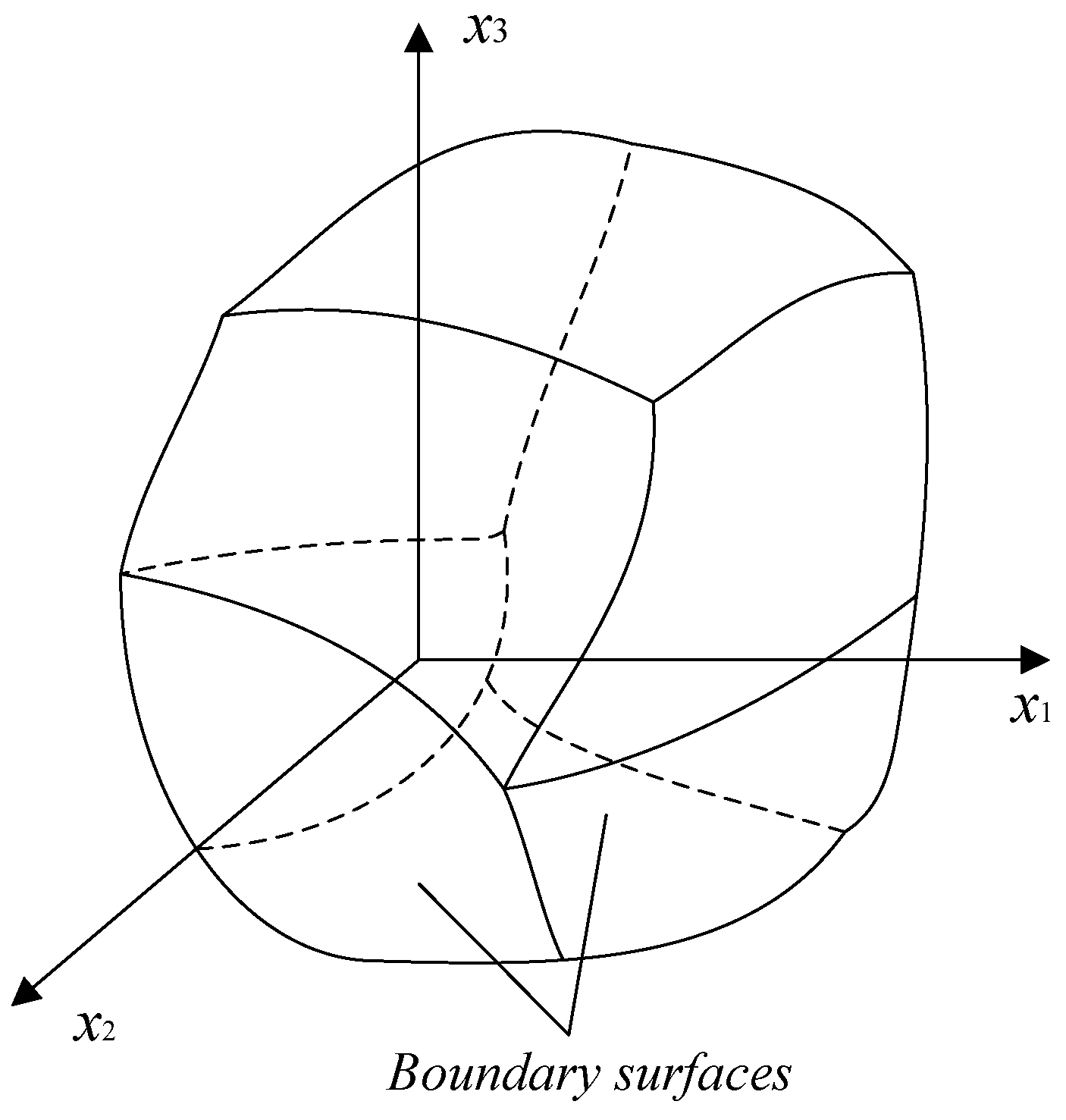
2.3. Definition of the Steady-State Security Region of an AC/DC Hybrid System

The steady-state security region of an AC/DC hybrid system is composed of the AC/DC system equality constraints of power flow equations, the AC system’s state and control variables’ constraints $h_1$, the LCC-HVDC system’s state and control variables’ constraints $h_2$, as well as the VSC-HVDC system’s state and control variables’ constraints $h_3$. To satisfy all these constraints, the steady-state security region is a set that is composed of the active power output and voltage amplitude of generators, complex power injection of load, and control variables of the HVDC system. Therefore, the steady-state security region Ω can be expressed as:

$$\mathsf{\Omega }=\{x|Equations(1)–(11),Inequalities(12)–(14)\}$$

(15)

where x denotes all control variables of the AC system and HVDC system (i.e. active power output and excitation voltage setting of generators, DC voltage, active power of HVDC, etc.), and the active power and reactive power of the load (including renewable energy). The set x can be viewed as a coordinate point in high dimensional space, which should satisfy Equations (1)–(14).

It is denoted that if X is the whole system’s electrical quantities which are constrained, it should satisfy:

$$X_{\min }\le X=g(x)\le X_{\max }$$

(16)

where $X_{\min }$ and $X_{\max }$ denote the vectors of lower bound and upper bound of X, respectively. g is the implicit functions of nonlinear power flow equations. When the inequality sign is translated into an equality sign, a plurality of high dimensional surfaces can be obtained. These high dimensional surfaces are defined as boundary surfaces of the steady-state security region.

Due to the nonlinearity of power flow equations, the steady-state security region is a high dimensional nonlinear geometry surrounded by a plurality of high dimensional surfaces in the Euclidean space. One variable in the set corresponds to one dimension of the space, and one constraint corresponds to one boundary. So, the steady-state security region consists of boundary surfaces corresponding to all constraints. If the operating point is inside the steady-state security region, it can be concluded that the system satisfies all constraints. Once the network’s topology and constraints are decided, the steady-state security region is uniquely determined. The schematic diagram of the steady-state security region is shown in Figure 1.

3. Characterization and Analysis of the Steady-State Security Region of an AC/DC System

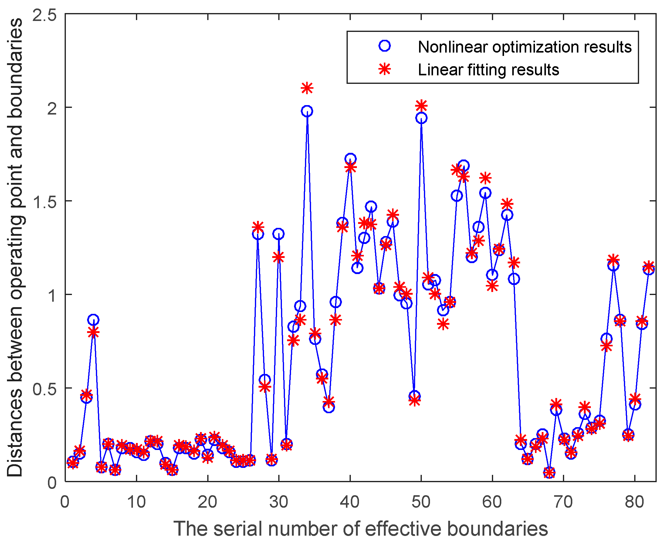
3.1. The Effective Boundaries Screening and the Solution of Distances between the Operating Point and the Effective Boundaries

One surface in the steady-state security region corresponds to one inequality constraint. On a certain region surface, the inequality constraint of the surface transforms into the equality constraint in this boundary, keeping the other inequality constraints satisfied. For example, the surface ${\omega }_k$ corresponding to the lower bound of the ignition angle can be expressed as:

$${\omega }_k=\{x\in \mathsf{\Omega }|\alpha ={\alpha }_{\min }\}$$

(17)

It is worth mentioning that only parts of boundaries are effective boundaries of the steady-state security region. If the Equation (17) is a null value, it means that this boundary is a non-effective boundary of the steady-state security region.

It is difficult to obtain the mathematical expressions of the boundaries of the steady-state security region (Equation (16)), as they are characterized by the nonlinear implicit inter-coupling functions. By using the hyper box region in References [6,7,8], the adjustment range of all control variables can be obtained, which, however, has some limitations. It cannot obtain the evolution process of the boundary and information of the global region, and the solution process is complex. Therefore, this paper employs the distance between the basic operating point and each surface to characterize the steady-state security region, which is able to achieve more accurate solutions, and reflect the global information. The distance can be also used as an evaluation index of safety control (i.e., preventive control and correction control [26]).

The distance of the steady-state security region of the AC/DC system is defined as the distance between the basic operating point $x_0$ and each effective boundary. It can be expressed as Equation (18).

$$d_k=\min \left|\right|x-x_0\left|\right|,x\in {\omega }_k$$

(18)

The larger the distance is, the greater the ranges are for the adjustment of the active power output and voltage amplitude of the generators and the control variables of the HVDC system, and the greater the allowable fluctuation range of the renewable energy or the load. To solve for the distance, the calculations can be converted to the following nonlinear optimization problems.

$$\begin{array}{l}{d}_k=\min \left|\right|x-x_0\left|\right|, x\in {\omega }_k\\ \begin{array}{cc}s.t.& \{\begin{array}{c}f(X)=0\\ \begin{array}{l}{h}_1(U_i,\mathrm{\Delta }{\theta }_{ij},P_g,P_{n+1},Q_{n+1})\le 0\\ h_2(\alpha ,\gamma ,U_d,I_d,P_d,Q_{d1},Q_{d2})\le 0\\ h_3(P_s,Q_s,U_s,I_s,M,\delta )\le 0\end{array}\\ An equality constraint\end{array}\end{array}\end{array}$$

(19)

where f is the equalities of power flow equations, X denotes all electrical quantities of the whole system, and ‘an equality constraint’ refers to the constraint corresponding to boundary ${\omega }_k$. If the optimization is not solvable, the corresponding boundary is a non-effective boundary.

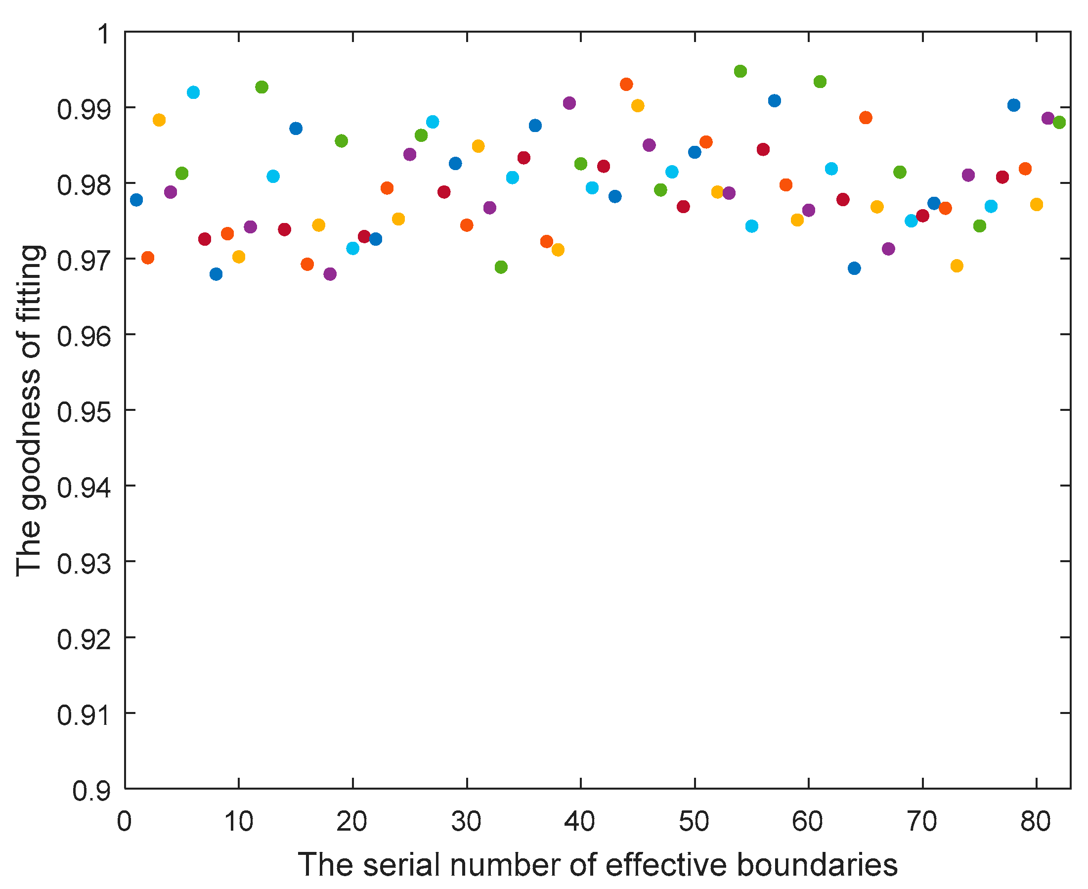
3.2. Regression of Effective Boundaries

Since the calculation speed of nonlinear optimization is slow, in order to adapt to the requirements of online calculation and fast safety analysis of power systems, the boundary surfaces can be expressed in linear regression equations based on the screening results obtained in Section 3.1. (It can be seen that the linear regression boundaries can replace the original boundary surfaces well from the case study below). For each effective boundary, the critical points are chosen randomly on the boundary surface based on the Equations (1)–(11), and the number of critical points is selected as 4–6 times the dimensions of the steady-state security region (the undetermined coefficients). According to the chosen critical points, the multiple linear regression is completed according to the regression Equation (20).

$${\displaystyle \sum _{i\in G}({\epsilon }_i{P}_i+{\chi }_i{U}_i)+}{\displaystyle \sum _{i\in L}({\eta }_i{P}_i+{\zeta }_i{Q}_i)+\lambda }{I}_d+\omega \gamma +\upsilon P_s+\tau U_s+\xi Q_{s1}+\psi Q_{s2}=1$$

(20)

The ${\epsilon }_i$、${\mathsf{\chi }}_i$、${\eta }_i$、${\zeta }_i$、$\lambda$、$\omega$、$\upsilon$、$\tau$、$\xi$ and $\psi$ are undetermined coefficients. G and L denote generators and loads, respectively. It is assumed that the LCC-HVDC is selected for constant current control and constant extinction angle control. The VSC-HVDC rectifier side adopts a constant active power and constant reactive power control, and the inverter side adopts a constant DC voltage and constant reactive power control. $Q_{s1}$ and $Q_{s2}$ are reactive power setting values of both sides of VSC converters.

The goodness of linear fitting can be characterized by R² value. It is assumed that $y_i$ represents the actual values of the undetermined coefficients of the fitting equation, ${\widehat{y}}_i$ denotes the actual values of the undetermined coefficients obtained by fitting, and $\overline{y}$ is the average value of the undetermined coefficients obtained by fitting. Also, it is defined that the quadratic sum of the total deviations is $TSS={\displaystyle \sum }{(y_i-\overline{y})}^2$, the quadratic sum of the regression is $ESS={\displaystyle \sum }{({\widehat{y}}_i-\overline{y})}^2$, and the quadratic sum of the residuals is $RSS={\displaystyle \sum }{(y_i-{\widehat{y}}_i)}^2$. The R² value of regression goodness can be formulated as:

$$R^2=\frac{ESS}{TSS}=1-\frac{RSS}{TSS}$$

(21)

However, with the increase of the number of critical points, the R² value of regression goodness will also increase. In order to eliminate the influence of the number of critical points on the regression goodness, the regression goodness is corrected to Equation (22):

$${\overline{R}}^2=1-\frac{RSS/(n-k-1)}{TSS/(n-1)}$$

(22)

where k is the number of variable coefficients to be determined, n − k − 1 is the free degree of the quadratic sum of residuals, and n − 1 is the free degree of the quadratic sum of the total deviations. The closer the value is to 1, the better the regression effect.

3.3. Safety Judgment of the Operating Point

The operating points can be divided into safe and unsafe operating points. On each side of the boundary surface, the operating points satisfy and dissatisfy the corresponding constraints, respectively. In the n-dimensional steady-state security region, it is defined that the coordinate point $(x_{10}$,$x_{20}$,……,$x_{n0})$ is the basic operating point of the steady-state security region.

The expression of the boundary surface obtained by linear regression can be transformed into $\mathrm{S}:a_1{x}_1+a_2{x}_2+\dots +a_n{x}_n+b=0$, where $a_1$, $a_2$, …, $a_n$ are the coefficients of expression, and $x_1$, $x_2$, …, $x_n$ are the dimension variables in space. For the boundary corresponding to the upper bound, the sign of b should be the same as the sign of the limit value of the constraint. For the boundary corresponding to the lower bound, the sign of b should be contrary to the sign of the limit value of the constraint. The judging standard that the operating point is safe is that all the effective boundary surfaces satisfy the equation below:

$$a_1{x}_{10}+a_2{x}_{20}+\cdots +a_n{x}_{n0}+b>0$$

(23)

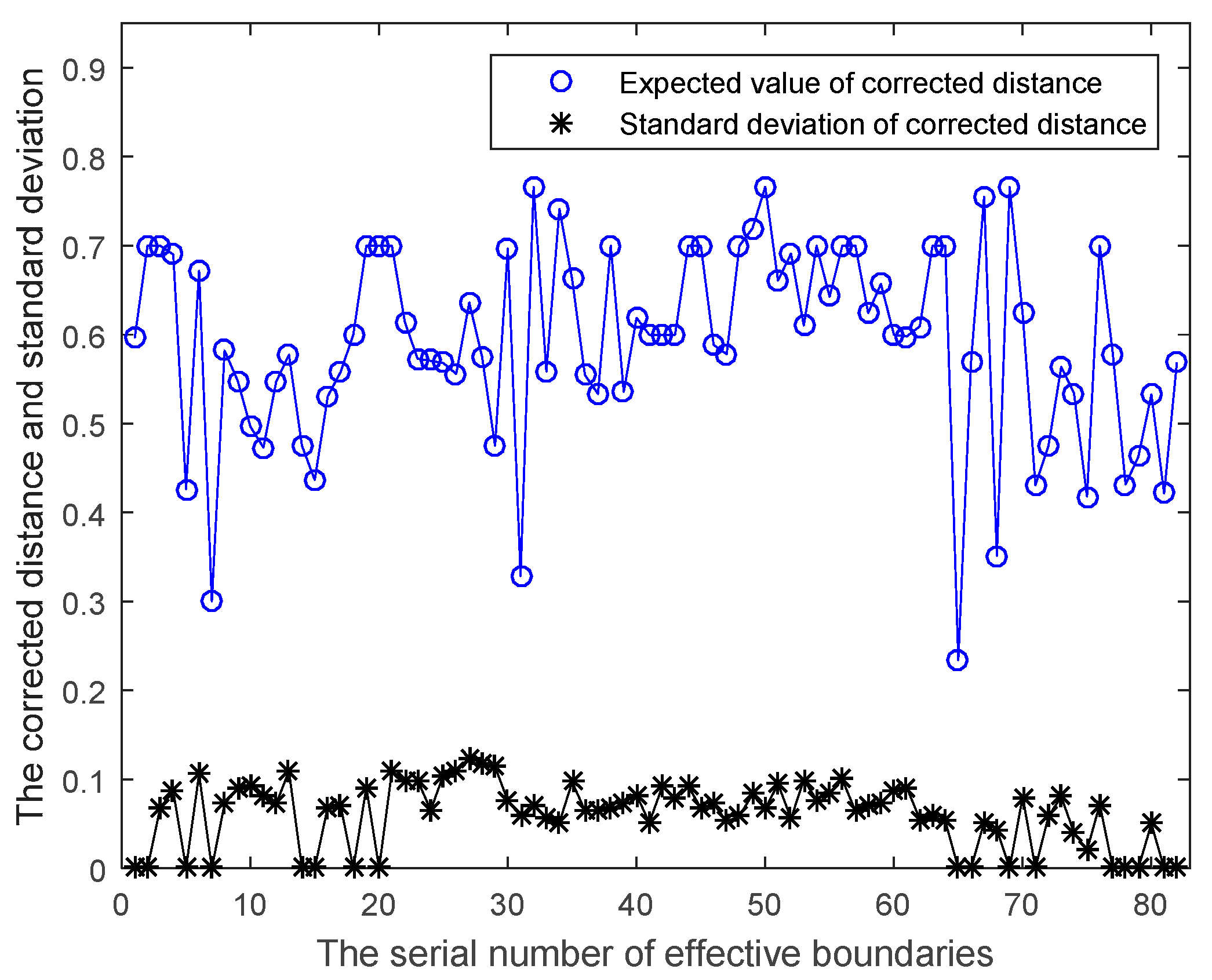
3.4. The Solution of Distance and Corrected Distance Based on the Regression Results

In order to obtain the physical meaning of distance, the transformation of boundary equations will be completed below. According to Equations (16) and (20), the linear fitting expression of each electrical quantity in the system can be formulated as:

$$X=C_1{x}_1+C_2{x}_2+\cdots C_n{x}_n+C_0$$

(24)

where X is the vector of the whole system electrical quantities, $C_1$,$C_2$,…,$C_n$ are the vectors of each dimension’s coefficients, and $C_0$ is the constant vector. The upper bounds and the lower bounds of the electrical quantities are substituted into Equation (24), and Equation (24) can be transformed into the boundary expression in Section 3.3.

On the basis of the expression of the boundary surface obtained by the method of linear regression in Section 3.2, the expression of the boundary surface can be translated into:

$$S:c_1{x}_1+c_2{x}_2+\cdots c_n{x}_n+c_0-e=0$$

(25)

Among them, $c_0$,$c_1$,…,$c_n$ are equal to the elements in $C_0$,$C_1$,…,$C_n$ corresponding to each boundary. Also, the e is the value of the upper or lower bound of the corresponding constraint. So, the distance between the operating point and the hyperplane in Euclidean space can be formulated by Equation (26):

$$d_i=\frac{|c_1{x}_{10}+c_2{x}_{20}+\cdots c_n{x}_{n0}+c_0-e|}{\sqrt{c_1^2+c_2^2+\cdots c_n^2}}$$

(26)

Since each dimension of the steady-state security region might use different units, the distances obtained above cannot be directly used to represent the system security margin. Therefore, the numerical value of each electrical quantity should be normalized. The meaning reflected in space is that the axes are stretched or compressed in geometric space, and then the steady-state security region is shifted. Supposing that the numerical range of each dimension variable is translated into 0–1, and as it is denoted that the $c_{i\max }$ and $c_{i\min }$ are the upper and lower bound of the i-th dimension variable, respectively, then the boundary surface can be represented as:

$$S:c_1(c_{1\max }-c_{1\min })x_1+c_{1\min }+c_2(c_{2\max }-c_{2\min })x_2+c_{2\min }+\cdots c_n(c_{n\max }-c_{n\min })x_n+c_0-e=0$$

(27)

The corrected distance can be calculated by:

$${\overline{d}}_i=\frac{|c_1(c_{1\max }-c_{1\min })x_{10}+c_2(c_{2\max }-c_{2\min })x_{20}+\cdots c_n(c_{n\max }-c_{n\min })x_{n0}+c_0+c_{1\min }+\cdots +c_{n\min }-e|}{\sqrt{c_1^2{(c_{1\max }-c_{1\min })}^2+c_2^2{(c_{2\max }-c_{2\min })}^2+\cdots c_n^2{(c_{n\max }-c_{n\min })}^2}}$$

(28)

The coordinate point (0.5, 0.5, ..., 0.5) can be viewed as the central point of the security region. If the corrected distances between the operating point and all boundaries are large, it means that the operating point is closer to the geometric center of the steady-state security region, and the higher the system’s security is, and the greater the operation margin. If the corrected distance between the operating point and the partial boundaries are small, it means that the constraint conditions corresponding to these boundaries have a large risk of exceeding the limits.

3.5. The Physical Meaning of the Corrected Distance

Denoting that $e_i$ = $c_i(c_{i\max }-c_{i\min })$, $e_0$ = $c_0+c_{1\min }+\cdots +c_{n\min }$, Equation (28) can be rewritten as:

$${\overline{d}}_i=\frac{|e_1{x}_{10}+e_2{x}_{20}+\cdots e_n{x}_{n0}+e_0-e|}{\sqrt{e_1^2+e_2^2+\cdots e_n^2}}$$

(29)

In the following text, ‘electrical quantity of constraint’ refers to the electrical quantity to be constrained corresponding to a certain boundary surface. It can be seen from the forms of Equations (24) and (29) that the physical meaning of molecular in Equation (29) is the available capacity of the electrical quantity of constraint in the current operating point. The available capacity is the difference between the limit value and the current value of the electrical quantity of constraint, which is consistent with the index of the traditional steady-state power flow security check. It can also be seen that the physical meaning of $e_i$ in the denominator of Equation (29) is the numerical variation of the electrical quantity of constraint when the value of the i-th dimension variable increases by one unit. So, the denominator characterizes the influence degree of the variations of all dimension variables on the electrical quantity of constraint, which reflects the comprehensive sensitivity between the electric quantity of constraint and all dimension variables. The traditional steady-state power flow security check does not have this index.

The traditional steady-state power flow security check can only reflect the difference between the bound value and the current value, and it cannot reflect the influence of the fluctuations of the dimensional variables on the electrical quantity of constraint. For example, when the difference between the current value and bound value of two branches’ power flow (the molecular in Equation (29)) are the same, it should be noticed that one branch’s comprehensive sensitivity (the denominator in Equation (29)) between the branch’s power flow and all dimension variables may be larger. Therefore, the fluctuations of the load or renewable energy on this branch’s power flow is more sensitive, thus this branch is less secure.

The corrected distance between the operating point and a boundary is large, which indicates that the constraint value corresponding to this boundary can be greatly utilized, or the fluctuations of dimension variables have little influence on the electrical quantity of constraint, or both. In the AC/DC system with large-scale intermittent energy, the physical meaning of the denominator in Equation (29) should be taken full advantage of. Therefore, the corrected distance can be used to characterize the vulnerability of the system, that is, the short links of the system.

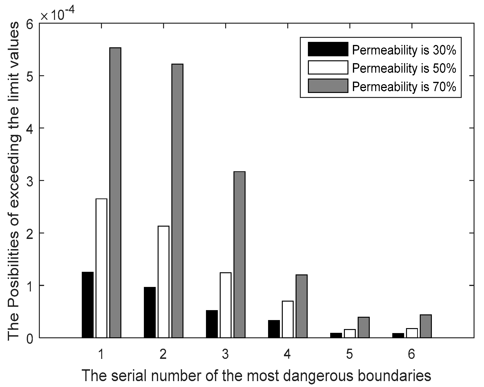
3.6. Probabilistic Analysis of Corrected Distance Considering the Fluctuations of Renewable Energy

The corrected distance between the operating point and the boundary surface can reflect the tolerance of the operating point to the fluctuations of interstitial energy. It is assumed that the fluctuations of the load and the renewable energy obey the normal distribution (taking normal distribution, for example, the results of other distributions can be obtained similarly), and the power imbalance is assumed by the balancing machine. Thus, the expected value of the corrected distance is the distance between the boundary and the operating point at which the expected value of distribution of each load or new energy is located. The standard deviation of normal distribution of the i-th renewable energy or load is denoted as ${\sigma }_i$. Hypothesizing that the probabilistic distribution of each load or renewable energy is independent of each other, the variance of the corrected distance ${\sigma }^2$ can be formulated as:

$${\sigma }^2={\displaystyle \sum _{i\in L}\frac{1}{e_1^2+e_2^2+\cdots e_n^2}(e_i^2{\sigma }_i^2)}$$

(30)

If the variances of normal distribution of renewable energy and load connected to one bus are different, the value of ${\sigma }_i$ should be firstly calculated in a similar manner.

Some boundaries’ corrected distances are large, while they may have larger variance. Therefore, under the fluctuations of new energy, the probability that their corrected distances are lower than the threshold may be larger. Therefore, the security of a boundary needs to be weighed by the expected value and variance of the corrected distance at the same time.

When the operating point is close to a boundary of the steady-state security region, the system’s security is greatly reduced, so the corrected distance’s threshold can be set as $d_0$. It is supposed that when the excepted value of corrected distance between the operating point and the i-th effective boundary is $d_{i0}$, the probability $P_{unsafe}^i$ that the corrected distance between the operating point and this boundary is lower than the threshold is:

$$P_{unsafe}^i={\displaystyle {\int }_{-\infty }^{d_0}\frac{1}{\sqrt{2\pi }\sigma }}{e}^{-\frac{{(y_i-d_{i0})}^2}{2{\sigma }^2}}d{y}_i$$

(31)

The probability $P_{unsafe}$ that there exists a distance below the threshold in all distances between the operating point and the boundary surfaces is:

$$P_{unsafe}=1-{\displaystyle \prod (1-P_{unsafe}^i)}$$

(32)

Equation (32) reflects the whole system’s security and invulnerability.

4. Case Study

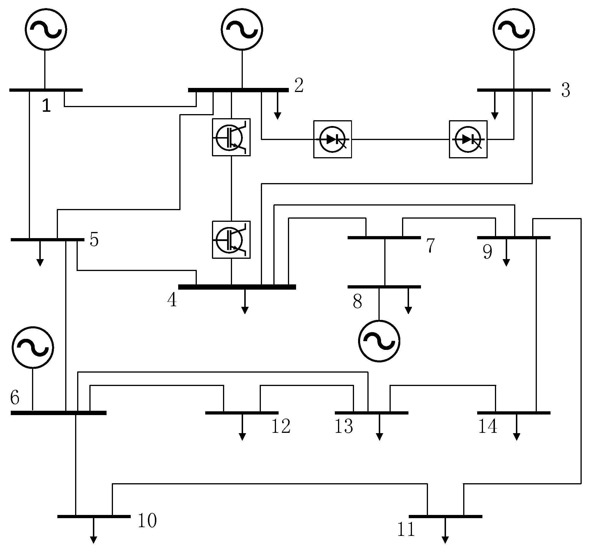
4.1. Example of IEEE14 Standard Test System

The standard IEEE14-bus system is examined in this case, as shown in Figure 2. The line 2–3 is replaced by a LCC-HVDC transmission line, and bus 2 is connected to the rectifier of the LCC-HVDC. The reactive power compensation is provided at both bus 2 and bus 3. The constant current control is chosen for the rectifier, and the constant extinction angle control is chosen for the inverter. The line 2–4 is replaced by a VSC-HVDC transmission line, and bus 2 is connected to the rectifier of the VSC-HVDC as well. The constant active and reactive power control is selected for the rectifier, and the constant DC voltage and reactive power control is selected for the inverter. The numbers in the Figure 2 indicate the bus serial number. The basic operating parameters of the LCC-HVDC and VSC-HVDC system are presented in

Table 1. Basic operating parameters of the LCC-HVDC (Line Commutated Converter-High Voltage Direct Current) system.

Quantity	Value
DC voltage	200 kV
DC current	350 A
Ignition angle	21.79°
Extinction angle	23.61°
Internal reactance	0.067 H
DC resistance	28.54 Ω
Filter capacitance	50 MVar
The ratio of converter transformers	1:1.2

and

Table 2. Basic operating parameters of the VSC-HVDC (Voltage Sourced Converter-High Voltage Direct Current) system.

Quantity	Value
DC voltage	200 kV
DC current	266.7 A
Reactive power of rectifier	−15.7 MVar
Reactive power of inverter	13.7 MVar
Commutation reactance	11.42 H
DC resistance	37.46 Ω
Modulation of rectifier	1.097
Phase shift angle of rectifier	1.5616°
Modulation of inverter	0.997
Phase shift angle of inverter	1.5947°

.

Dimensions of the steady-state security region include the active power output and voltage amplitude of all generators except for slack machine, the active and reactive power of the load (including renewable energy), the set values of DC current and extinction angle of the LCC-HVDC system, and the set values of active and reactive power and DC voltage of the VSC-HVDC system. The total dimension is 36.

The limitation values are given in

Table 3. The values of upper and lower limitations of constraint.

Quantity	Upper Bound	Lower Bound
Bus voltage	1.15	0.95
Phase difference of line	15°	−15°
Active power of balancing machine	5	0
Reactive power of balancing machine	2.5	−2.5
DC voltage of LCC-HVDC	1.8	1.2
DC current of LCC-HVDC	0.6	0.1
Ignition angle	50°	5°
Extinction angle	35°	15°
Reactive power compensation capacity	0.8	0
DC voltage of VSC-HVDC	1.6	1.0
DC current of VSC-HVDC	0.6	0.1
Phase shift angle	3°	0°
Modulation of inverter	1.4	0
Reactive power setting value of VSC-HVDC	1	−1
Active power setting value of VSC-HVDC	1.1	0

. The following values are normalized (the base capacity is 100 MVA, and the base voltage is 138 kV).

This 36-dimensional steady-state security region is formed by 102 boundary surfaces, but only some of them are effective boundaries that constitute the steady-state security region geometry. The AC/DC power flow is calculated by using the test system standard data and the data in Table 1 and Table 2, and the steady-state operating point of the system is obtained. The distances between the steady-state operating point and all effective boundary surfaces can be computed by Equation (19).

Most of the AC system constraints and parts of the HVDC system constraints form the effective boundaries. The total number of effective boundaries is 82. Then, the critical points on the boundary surfaces were generated randomly. The number of the critical points is 216. The linear regression was completed by Equation (20).

Based on the results of the expressions obtained by linear regression, the test point is a safe point calculated by Equation (23). Then, the distances between the operating point and hyperplanes were calculated by Equation (26).

The distances between the operating point and all effective boundaries calculated by Equations (19) and (26) are shown in Figure 3.

The ${\overline{R}}^2$ value of goodness of fitting is calculated by Equation (22). Also, the ${\overline{R}}^2$ value of goodness of fitting of each effective boundary is shown in Figure 4.

It can be seen from Figure 3 and Figure 4 that the results of linear fitting are of higher accuracy, so the linear hyper planes can be used to instead of the original boundary surfaces of the steady-state security region.

Based on the results obtained by the linear regression, the corrected distances were calculated by Equation (28). The corrected distances between the operating point and all effective boundaries are shown in Figure 5.

It is assumed that the fluctuations of load and renewable energy obey the normal distribution, and the probability distribution of each load or renewable energy is independent of each other. The expected value of the active power and reactive power of load or new energy are chosen as the values of the tested system. Furthermore, the variance of the active power and reactive power of load or new energy in corrected space is assumed as 0.015. The standard deviations of the corrected distances of all effective boundaries can be calculated by Equation (30), which are also shown in Figure 5.

It can be seen that most of the corrected distances range from 0.3 to 0.7, which means that the operating point is relatively close to the geometric center of the steady-state security region. However, some boundaries have small corrected distances. This means that the operating point has a great risk of exceeding the limit of constraints corresponding to these boundaries. It should also be noticed that some boundaries have large corrected distance, while their variances are small. This means that the operating points also have a great risk of exceeding the limits of these boundaries. Therefore, the security of a boundary needs to be weighed by the corrected distance and their variance at the same time.

It is assumed that the threshold of corrected distance is 0.20. The possibility that the distance between the operating point and the boundary is lower than the threshold was calculated by Equation (31).

The 10 boundaries that have lowest corrected distances and their standard deviations and probabilities of unsafety are presented in

Table 4. Calculation results of the boundaries which have the lowest corrected distances.

Effective Boundary	Corrected Distance	Standard Deviation	Probability of Unsafety
Upper bound of DC current of LCC	0.2340	0	0
Upper bound of voltage amplitude of bus 8	0.3000	0	0
Upper bound of phase angle difference of line 1–5	0.3214	0.0589	0.0144
Lower bound of ignition angle	0.3514	0.0438	2.736 × 10−4
Upper bound of DC current of VSC	0.4178	0.0363	3.606 × 10−8
Lower bound of reactive injection of rectifier	0.4215	0.0521	1.342 × 10−5
Upper bound of voltage amplitude of bus 6	0.4265	0	0
Lower bound of extinction angle	0.4305	0	0
Upper bound of reactive injection of inverter	0.4315	0.0398	9.721 × 10−8
Lower bound of voltage amplitude of bus 3	0.4367	0	0

.

The shortest distance between the operating point and the effective boundaries is 0.2340 (upper bound of DC current of LCC). This means that if the adjustment range of the control variables is large, and the operating point has a large probability of exceeding this boundary surface. However, because its standard deviation is zero, so it will not be out of limitation under the fluctuations of load or renewable energy. Therefore, if the uncertainty of load or renewable energy needs to be considered, the index of standard deviation should be employed.

Furthermore, the 10 boundaries that have greatest probabilities for a corrected distance below threshold and their corrected distances and standard deviations are presented in

Table 5. Calculation results of the riskiest restraint conditions.

Effective Boundary	Probability of Unsafety	Corrected Distance	Standard Deviation
Upper bound of phase angle difference of line 1–5	0.0144	0.3214	0.0589
Upper bound of reactive power of balancing node	0.0042	0.4750	0.1043
Upper bound of voltage amplitude of bus 11	8.017 × 10−4	0.4966	0.0904
Upper bound of voltage amplitude of bus 12	4.977 × 10−4	0.4729	0.0829
Lower bound of ignition angle	2.736 × 10−4	0.3514	0.0438
Upper bound of voltage amplitude of bus 10	5.614 × 10−5	0.5484	0.0902
Upper bound of phase angle difference of line 7–9	2.955 × 10−5	0.5357	0.0834
Lower bound of reactive injection of rectifier	1.342 × 10−5	0.4215	0.0521
Lower bound of voltage amplitude of bus 4	1.322 × 10−5	0.5307	0.0691
Upper bound of phase angle difference of line 5–6	2.387 × 10−6	0.5333	0.0648

.

It can be seen that the constraint condition for which the operating point has the greatest probability of exceeding the threshold is the upper bound of phase angle difference of line 1–5 under the fluctuations of renewable energy, while its corrected distance is not the lowest distance. From Table 5, it can also be seen that some boundaries have a low possibility of unsafety, but these boundaries did not appear in Table 4. It can also be seen that the constraints of the AC system are more “dangerous” than the ones of the DC system.

Therefore, if the fluctuations of load or renewable energy are not considered, the index of corrected distance is enough to analyze the system’s security. If the probability characteristics of load or renewable energy should be considered to analysis the unsafety probability of constraints and the whole system, the index of standard deviation ought to be considered.

Moreover, the whole system’s unsafety probability can be calculated by Equation (32), which results in a value of 0.0252.

The conventional power flow security check can only give the calculation values of electrical variables and their comparisons with the constraint values, and it is difficult to give the operating margin values. This method can give the safety information feedback from the view of geometry when the AC/DC system operates in static state.

It can be seen from Figure 5 that the corrected distances between the operating point and the boundaries corresponding to nodal voltage constraints or the boundaries corresponding to the HVDC system’s constraints are closer than the boundaries corresponding to the line phase angle difference constraints. Therefore, it can be approximately concluded that the deviation degree between the operating point and the geometric center is relatively large in these dimensions. Also, it can be seen from Table 4 that it is more prone to exceed the limit of these constraints when the adjustment range of the control variables is large or large-scale fluctuations in renewable energy sources and load occur.

For all variables, the probabilities that the corrected distance below the threshold are greatest in the dimensions of the upper bound of phase angle difference of line 1–5 and the upper bound of the reactive power output of the balancing machine. Hence, it is necessary to improve the branch flow capacity of line 1–5 and the reactive power upper limit of the balancing machine. Considering the geometrical characteristic of the steady-state security region, all control variables can be controlled coordinately to pull the operating point to the geometric center so as to ensure an adequate steady-state operating margin in the event that a large amount of renewable energy connects to the grid.

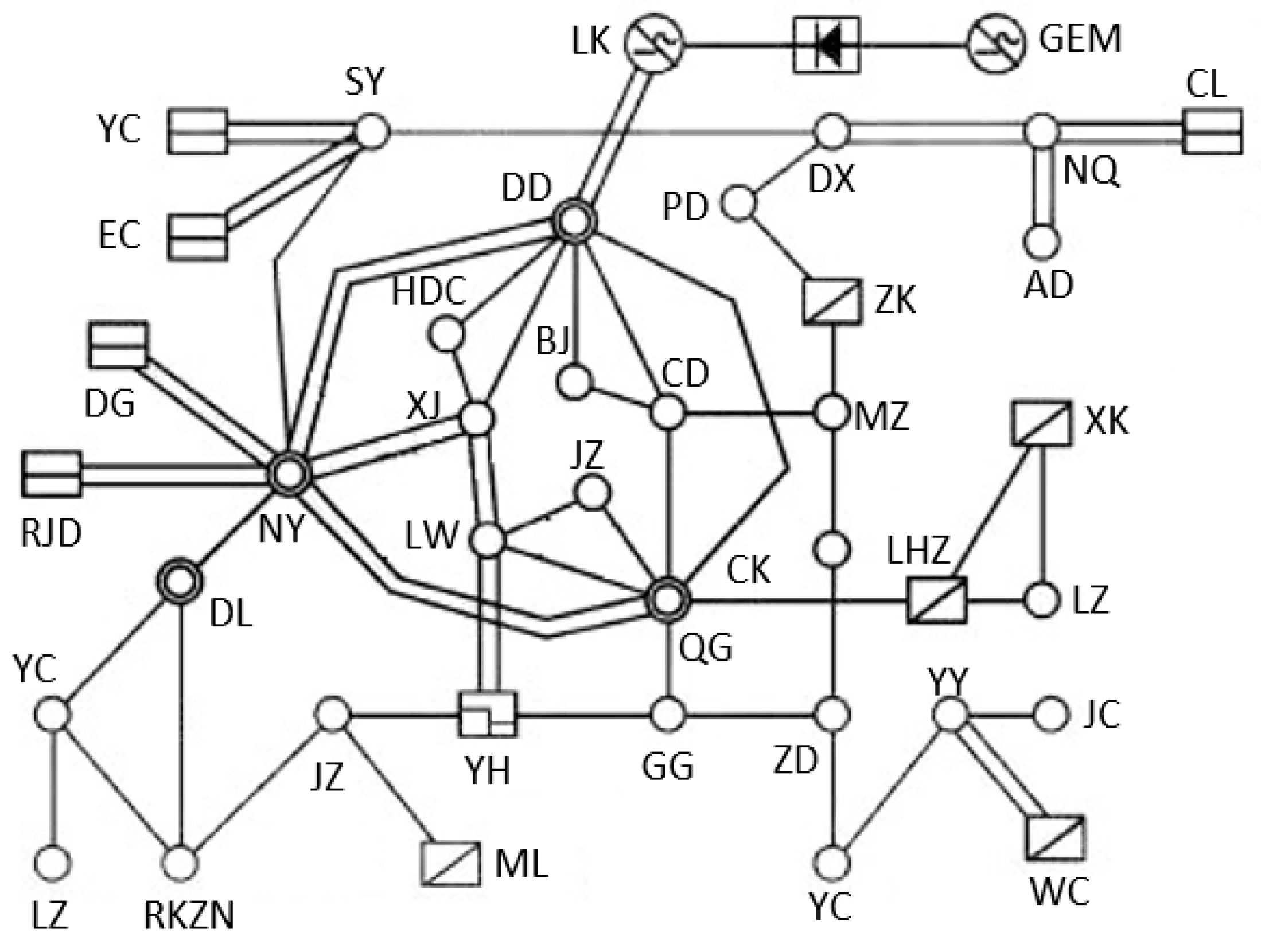
4.2. Example of Actual Power Grid

Taking a power grid in Western China as an example, each station is equivalent to an equivalent power supply, in which a bipolar single bridge LCC-HVDC transmission line and a VSC-HVDC transmission line are parallel between the LK station and the GEM station, as shown in Figure 6.

By repeating the above work, 172 effective boundaries are screened. It is assumed that the standard deviation of the normal distribution of renewable energy is twice that of the load, and the threshold of corrected distance is 0.15. When the permeability of renewable energy is 30%, the possibilities of exceeding the limit values were calculated by Equation (31). The effective boundaries corresponding to the six lowest unsafety probabilities (the riskiest boundaries) are the upper bound of bus voltage in NY station, upper bound of phase angle difference between NY station and DL station, lower bound of bus voltage in LZ station, upper bound of bus voltage in SY station, lower bound of bus voltage in RKZN station, and lower bound of ignition angle, respectively (the serial numbers of abscissa 1–6 in Figure 7, respectively). The security of these boundaries needs to be paid enough attention.

Then, the permeability of renewable energy is increased to 50% and 70%. The above work was repeated, respectively. The unsafety probabilities corresponding to the most "dangerous" constraint conditions under different permeability are shown in Figure 7.

The whole system’s unsafety probability can be calculated by Equation (32), the values for which are 0.000358, 0.000964, and 0.002537, respectively.

With the increase of permeability of renewable energy, the whole system’s unsafety probability and each constraint’s unsafety probability will all increase sharply. Therefore, system dispatchers or system designers can use these methods to find the weak links of an AC/DC system so as to ensure an adequate steady-state operating margin in the event that a large amount of renewable energy connects to the grid.

5. Conclusions

In this paper, the definition and description of the steady-state security region of an AC/DC hybrid power system are presented to extend the application of the conventional steady-state security region. Since the boundaries of the steady-state security region cannot be expressed by the mathematical expressions accurately, the screening method of effective boundary surfaces, the calculation of distances and corrected distances between steady-state operating point and effective boundary surfaces, the safety judging method of operating points, the physical meaning of corrected distance, and the probabilistic analysis of corrected distance considering the fluctuations of renewable energy are proposed in this paper, in order to ensure that the solution of the security region can accurately reflect the global security information and weak links of the power system. In addition, considering the uncertainty of intermittent energy, the case study reveals that the system’s steady-state security region can be characterized by the expected values and standard deviations of the corrected distances and the probability that the corrected distances are lower than threshold. The proposed methods are effective in the security analysis of the AC/DC system with a large amount of renewable energy.

References

1. Zeng, X.J.; Yu, Y.X.; Huang, C.H. Steady-state security region (SSR) and its visualization of bulk high voltage power system. In Proceedings of the International Conference on Power System Technology, Kunming, China, 13–17 October 2002; pp. 1259–1263. [Google Scholar]
2. Xiao, J.; Su, B.Y.; Li, X.; Wang, C.S. Secure region of network and comparison with invulnerability. Complex Syst. Complex. Sci. 2016, 4, 41–50. [Google Scholar]
3. Galiana, F.D. Analytic properties of the load flow problem. In Proceedings of the International Symposium on Circuits System Special Session on Power System, Philadelphia, PA, USA, 5–7 May 1977; pp. 802–816. [Google Scholar]
4. Galiana, F.D.; Lee, K. On the steady stability of power system. In Proceedings of the Power Industry Computer Applications Conference, Toronto, ON, Canada, 9–10 January 1977; pp. 201–210. [Google Scholar]
5. Jarjis, J.; Galiana, F.D. Quantitative analysis of steady state stability in power networks. IEEE Trans. Power Appar. Syst. 1981, PAS-100, 318–326. [Google Scholar] [CrossRef]
6. Felix, F.W. Steady-state secutity regions of power systems. IEEE Trans. Circuits Syst. 1982, 29, 703–711. [Google Scholar]
7. Yu, Y.X.; Feng, F. Active power steady-state security region of power system. Sci. China Ser. A 1990, 33, 664–672. [Google Scholar]
8. Huang, C.H.; Yu, Y.X.; Ge, S.Y. Reactive power steady state security region. J. Tianjin Univ. 1987, 8, 77–86. [Google Scholar]
9. Hnyilina, E.; Lee, S.T.Y.; Schweppe, F.C. Steady-state security regions: The set-theoretic approach. In Proceedings of the PICA Conference, Vancouver, BC, Canada, 28–31 May 1975; pp. 347–355. [Google Scholar]
10. Fischl, R.; DeMaio, J.A. Fast identification of the steady-state security regions for power system security enhancement. In Proceedings of the IEEE PES Winter Meeting, Detroit, MI, USA, 11–15 January 1976. Paper No. A76-076-0. [Google Scholar]
11. Chen, S.J.; Chen, Q.X.; Xia, Q. Steady-state security assessment method based on distance to security region boundaries. IET Gener. Transm. Distrib. 2013, 7, 288–297. [Google Scholar] [CrossRef]
12. Chen, S.J.; Chen, Q.X.; Xia, Q. N−1 security assessment approach based on the steady-state security distance. IET Gener. Transm. Distrib. 2015, 9, 2419–2426. [Google Scholar] [CrossRef]
13. Hu, L.L.; Zhao, J.L.; Jia, H.J.; Guo, X.L.; Zeng, Q. Computing the boundary of simple power system feasible region based on the optimization method. In Proceedings of the Innovative Smart Grid Technologies—Asia (ISGT Asia), Tianjin, China, 21–24 May 2012; pp. 1–6. [Google Scholar]
14. Yao, R.; Liu, F.; He, G.Y.; Fang, B.; Huang, L. Static security region calculation with improved CPF considering generation regulation. In Proceedings of the 2012 IEEE International Conference on Power System Technology (POWERCON), Auckland, New Zealand, 30 October–2 November 2012; pp. 1–6. [Google Scholar]
15. Rault, P.; Guillaud, X.; Colas, F. Investigation on interactions between AC and DC grids. In Proceedings of the 2013 IEEE Grenoble Conference, Grenoble, France, 16–20 June 2013; pp. 1–6. [Google Scholar]
16. Fan, J.C. Dynamic Security Region for AC/DC Parallel System and its Critical Cutset Representation. Ph.D. Thesis, Tianjing University, Tianjin, China, 2005. [Google Scholar]
17. Wang, C.C. Practical Dynamic Security Regions of AC/DC Parallel Systems to Guarantee Short-term Voltage Stability of Large Disturbance. Master’s Thesis, Tianjing University, Tianjin, China, 2007. [Google Scholar]
18. Shao, C.; Wang, X.; Shahidehpour, M.; Wang, X.; Wang, B. Power system economic dispatch considering steady-state secure region for wind power. IEEE Trans. Sustain. Energy 2017, 1, 268–278. [Google Scholar] [CrossRef]
19. Cheng, F.; Yang, M.; Han, X.; Liang, J. Real-time dispatch based on effective steady-state security regions of power systems. In Proceedings of the 2014 IEEE PES General Meeting—Conference & Exposition, National Harbor, MD, USA, 27–31 July 2014; pp. 1–5. [Google Scholar]
20. Chen, S.J.; Chen, Q.X.; Xia, Q. Steady-state security distance: Concept, model and meaning. Proc. CSEE 2015, 35, 600–608. (In Chinese) [Google Scholar]
21. Kundur, P. Power System Stability and Control; McGraw-Hill Education: New York, NY, USA, 1994; pp. 463–576. [Google Scholar]
22. Ni, Y.X.; Chen, S.S.; Sun, B.L. Theory and Analysis of Dynamic Power System; Tsinghua University Press: Beijing, China, 2002; pp. 106–117. [Google Scholar]
23. Kim, C.K.; Sood, V.K.; Jang, G.S. HVDC Transmission: Power Conversion Applications in Power Systems; John Wiley & Sons: Singapore, 2009; pp. 125–186. [Google Scholar]
24. Sood, V.K. HVDC and Facts Controllers-Applications of Static Converters in Power Systems; Springer Science & Business Media: Boston, MA, USA, 2004; pp. 49–65. [Google Scholar]
25. Muhammad, H.R. Power Electronics: Circuits, Devices, and Applications, 3rd ed.; Pearson Education: New Delhi, India, 2004; pp. 226–303. [Google Scholar]
26. Dy-Liacco, T.E. Real time computer control of power system. Proc. IEEE 1974, 62, 884–891. [Google Scholar] [CrossRef]
Figure 1. Schematic diagram of the steady-state security region.
Energies 10 01181 g001
Figure 2. IEEE14-bus AC/DC hybrid system after transforming.
Energies 10 01181 g002
Figure 3. The distances between the operating point and all effective boundaries.
Energies 10 01181 g003
Figure 4. The R2 value of goodness of fitting of each effective boundary.
Energies 10 01181 g004
Figure 5. The corrected distances of all effective boundaries and their variances.
Energies 10 01181 g005
Figure 6. Geographic connection of the grid.
Energies 10 01181 g006
Figure 7. Comparison of operation margin before and after adjustment.
Energies 10 01181 g007