Single-Phase Autonomous Induction Generator with Single-Phase Rotor

Abstract

An autonomous induction generator (IG) with an asymmetric configuration, in which both the stator and the rotor are single-phase, is often formed when a triple-phase wound rotor loses connection to a winding component while running. The machine still works and is shown to be capable of generating modulated waveforms. Equations can help as an IG design guideline. The first harmonics of the mutual inductance effect on the IG is explained by its steady-state equivalent circuit.

1. Introduction

This work is a continuation and refinement of Professor Raul Rabinovici and Doctor Nathan Ben Hail’s article, “Autonomous Induction Generator with Single-Phase Rotor” [1]. In this paper, more exact formulae are developed and the resulting system is analyzed and shown to be capable of behaving with each of the six solutions. Furthermore, after the first analytical section, an additional simulation section was added, in which it is proved that the basic prediction of the analytical section also holds in a numerical simulation.

During recent decades, the wound rotor induction generator (IG) has been used more and more in applications such as wind turbines [2], water turbines [3], and mostly in small, portable autonomous configurations, such as the type small construction teams frequently use. Generally, the IG works autonomously while it is connected to a capacitor bank. Its operation is explained by a resonance phenomenon between the capacitor bank and the inductive components of the IG itself. When such a generator loses a phase connection, it does not cease operation, but rather provides distorted wave form while the resonance limits the effect of higher frequencies emanating from the rotor’s current asymmetrical connection. This article is about the effect of the first harmonics of the mutual inductance of the rotor and a single-phase stator coil under such conditions.

2. Induction Machine Model

The circuit of the induction machine model is shown in Figure 1. It is supposed that the IG rotates at a constant angular speed, $\mathsf{\omega }$. If the IG has $\mathrm{P}$ pole pairs, the electrical angular frequency of the rotor will be ${\mathsf{\omega }}_{\mathrm{r}}=\mathrm{P}\mathsf{\omega }$. The IG has the following mathematical model ([4], p. 197):

$${\mathrm{i}}_{\mathrm{s}}=-\mathrm{C}\frac{\mathrm{dv}}{\mathrm{dt}}$$

(1)

$$\mathrm{v}\left(\mathrm{t}\right)={\mathrm{R}}_{\mathrm{s}}{\mathrm{i}}_{\mathrm{s}}\left(\mathrm{t}\right)+{\mathrm{L}}_{\mathrm{s}}\frac{{\mathrm{di}}_{\mathrm{s}}\left(\mathrm{t}\right)}{\mathrm{dt}}+\frac{\mathrm{dm}\left(\mathrm{t}\right){\mathrm{i}}_{\mathrm{r}}\left(\mathrm{t}\right)}{\mathrm{dt}}$$

(2)

$$0={\mathrm{R}}_{\mathrm{r}}{\mathrm{i}}_{\mathrm{r}}\left(\mathrm{t}\right)+{\mathrm{L}}_{\mathrm{r}}\frac{{\mathrm{di}}_{\mathrm{r}}\left(\mathrm{t}\right)}{\mathrm{dt}}+\frac{\mathrm{dm}\left(\mathrm{t}\right){\mathrm{i}}_{\mathrm{s}}\left(\mathrm{t}\right)}{\mathrm{dt}}$$

(3)

where ${\mathrm{i}}_{\mathrm{s}}$ is the stator current, ${\mathrm{i}}_{\mathrm{r}}$ is the rotor current, v is the stator output voltage, is the stator circuit resistance, ${\mathrm{R}}_{\mathrm{r}}$ is the rotor circuit resistance, ${\mathrm{L}}_{\mathrm{s}}$ is the stator winding inductance, ${\mathrm{L}}_{\mathrm{r}}$ is the rotor winding inductance, C is the external capacitor (an external capacitor bank is necessary for any IG to work [5]), and m(t) is the mutual inductance between the stator and the rotor windings. If the stator and the rotor have sinusoidal distribution, the mutual inductance will also be sinusoidal ([6], pp. 80–108).

$$\mathrm{m}\left(\mathrm{t}\right)=\mathrm{Mcos}\left({\mathsf{\omega }}_{\mathrm{r}}\mathrm{t}\right)$$

(4)

Then, Equation (3) can be solved with an (indefinite) integral solution for ${\mathrm{i}}_{\mathrm{r}}\left(\mathrm{t}\right)$.

$${\mathrm{i}}_{\mathrm{r}}=-\frac{1}{{\mathrm{L}}_{\mathrm{r}}}{\mathrm{e}}^{-\frac{{\mathrm{R}}_{\mathrm{r}}}{{\mathrm{L}}_{\mathrm{r}}}\mathrm{t}}{{\displaystyle \int }}^{\text{}}{\mathrm{e}}^{\frac{{\mathrm{R}}_{\mathrm{r}}}{{\mathrm{L}}_{\mathrm{r}}}\mathrm{t}}{\mathrm{dmi}}_{\mathrm{s}}$$

(5)

Note the ${\mathrm{e}}^{-\frac{{\mathrm{R}}_{\mathrm{r}}}{{\mathrm{L}}_{\mathrm{r}}}\mathrm{t}}$ term. This is a phase shift effect between ${\mathrm{i}}_{\mathrm{r}}$ and ${\mathrm{mi}}_{\mathrm{s}}$. When $\frac{{\mathrm{R}}_{\mathrm{r}}}{{\mathrm{L}}_{\mathrm{r}}}$ approaches zero, then ${\mathrm{i}}_{\mathrm{r}}$ and ${\mathrm{mi}}_{\mathrm{s}}$ will tend to align. When $\frac{{\mathrm{R}}_{\mathrm{r}}}{{\mathrm{L}}_{\mathrm{r}}}\to \infty$ the phase shift will approach $90°$.

3. Approximate Solution of the System

The system of equations of the IG is usually used to perform a computer simulation rather than to obtain an analytical solution. However, the latter, although approximate, can contribute to a general understanding of the IG characteristics.

The analytical solution is obtained in this section for the steady-state case. It is supposed that in the steady-state condition, the stator current is a sinusoidal wave. This supposition is further validated by the experimental results, where the fundamental harmonic is taken into consideration. Furthermore, the stator circuit is an RLC circuit, a circuit consisting of a resistor (R), an inductor (L), and a capacitor (C), which attenuates high harmonics. Therefore, the stator current is deemed to be of the form ${\mathrm{i}}_{\mathrm{s}}\left(\mathrm{t}\right)={\mathrm{I}}_{\mathrm{s}}\mathrm{Cos}\left({\mathsf{\omega }}_{\mathrm{e}}\mathrm{t}\right)$, where ${\mathsf{\omega }}_{\mathrm{e}}$ is the stator currents wave frequency. From here, using this approximation:

$$\mathrm{m}\left(\mathrm{t}\right){\mathrm{i}}_{\mathrm{s}}\left(\mathrm{t}\right)=\frac{{\mathrm{MI}}_{\mathrm{s}}}{2}\left(\cos \left({\mathsf{\omega }}_{\mathrm{r}}+{\mathsf{\omega }}_{\mathrm{e}}\right)\mathrm{t}+\cos \left({\mathsf{\omega }}_{\mathrm{r}}-{\mathsf{\omega }}_{\mathrm{e}}\right)\mathrm{t}\right)$$

(6)

Therefore:

$$\frac{\mathrm{d}\left(\mathrm{m}\left(\mathrm{t}\right){\mathrm{i}}_{\mathrm{s}}\left(\mathrm{t}\right)\right)}{\mathrm{dt}}=-\frac{{\mathrm{MI}}_{\mathrm{s}}}{2}\left(\left({\mathsf{\omega }}_{\mathrm{r}}+{\mathsf{\omega }}_{\mathrm{e}}\right)\sin \left({\mathsf{\omega }}_{\mathrm{r}}+{\mathsf{\omega }}_{\mathrm{e}}\right)\mathrm{t}+\left({\mathsf{\omega }}_{\mathrm{r}}-{\mathsf{\omega }}_{\mathrm{e}}\right)\sin \left({\mathsf{\omega }}_{\mathrm{r}}-{\mathsf{\omega }}_{\mathrm{e}}\right)\mathrm{t}\right)$$

(7)

As such, Equation (3) can be solved with aid of the known indefinite integral: ${{\displaystyle \int }}^{\text{}}{\mathrm{e}}^{\mathsf{\alpha }\mathrm{t}}\sin \left(\mathsf{\beta }\mathrm{t}\right)\mathrm{dt}=\frac{{\mathrm{e}}^{\mathsf{\alpha }\mathrm{t}}\left(\mathsf{\alpha }\sin \left[\mathsf{\beta }\mathrm{t}\right]-\mathsf{\beta }\cos \left[\mathsf{\beta }\mathrm{t}\right]\right)}{{\mathsf{\alpha }}^2+{\mathsf{\beta }}^2}$, however, this is not an absolute form. It is correct to use only if the machine is assumed to work from time −$\infty$. This is an approximation, which was used in Reference [1]. It is hereby suggested to refine this approximation by using an absolute integral.

To acquire an absolute (for a finite time) integral, the integral

$${{\displaystyle \int }}_{\mathrm{k}}^{\mathrm{t}}{\mathrm{e}}^{\mathrm{as}}\sin \left(\mathrm{bs}\right)\mathrm{ds}=\frac{{\mathrm{e}}^{\mathrm{ak}}\left(\mathrm{bcos}\left(\mathrm{bk}\right)-\mathrm{asin}\left(\mathrm{bk}\right)\right)+{\mathrm{e}}^{\mathrm{at}}\left(-\mathrm{bcos}\left(\mathrm{bt}\right)+\mathrm{asin}\left(\mathrm{bt}\right)\right)}{{\mathrm{a}}^2+{\mathrm{b}}^2}$$

(8)

is evaluated. Now, another well-known trigonometric identity is used:

$${\mathrm{e}}^{\mathrm{ak}}\left(\mathrm{bcos}\left[\mathrm{bk}\right]-\mathrm{asin}\left[\mathrm{bk}\right]\right)=-{\mathrm{e}}^{\mathrm{ak}}\cdot \mathrm{a}\left(\sin \left[\mathrm{bk}\right]-\frac{\mathrm{b}}{\mathrm{a}}\cos \left[\mathrm{bk}\right]\right)=-{\mathrm{e}}^{\mathrm{ak}}\cdot \mathrm{a}\left(\frac{\sin \left[\mathrm{bk}-\arctan (\frac{\mathrm{b}}{\mathrm{a}})\right]}{\cos \left[\arctan [\frac{\mathrm{b}}{\mathrm{a}}]\right]}\right)$$

(9)

meaning, ${\mathrm{e}}^{\mathrm{ak}}\left(\mathrm{asin}\left[\mathrm{bk}\right]-\mathrm{bcos}\left[\mathrm{bk}\right]\right)={\mathrm{e}}^{\mathrm{ak}}\cdot \mathrm{a}\left(\frac{\sin \left[\mathrm{bk}-\arctan (\frac{\mathrm{b}}{\mathrm{a}})\right]}{\cos \left[\arctan [\frac{\mathrm{b}}{\mathrm{a}}]\right]}\right)$. If one wishes to zero the contribution of the constant, k, in the equation, then:

$$\mathrm{k}=\frac{1}{\mathrm{b}}\arctan \left[\frac{\mathrm{b}}{\mathrm{a}}\right](\pm \mathsf{\pi }\cdot \frac{\mathrm{n}}{\mathrm{b}})$$

(10)

Note ${\mathrm{i}}_{\mathrm{r}}\left(\mathrm{t}\right)=-\frac{1}{{\mathrm{L}}_{\mathrm{r}}}{\mathrm{e}}^{-\frac{{\mathrm{R}}_{\mathrm{r}}}{{\mathrm{L}}_{\mathrm{r}}}\mathrm{t}}{{\displaystyle \int }}^{\text{}}{\mathrm{e}}^{\frac{{\mathrm{R}}_{\mathrm{r}}}{{\mathrm{L}}_{\mathrm{r}}}\mathrm{t}}{\mathrm{dmi}}_{\mathrm{s}}$ and ${\mathrm{dmi}}_{\mathrm{s}}=-\frac{{\mathrm{MI}}_{\mathrm{s}}}{2}\left(\left({\mathsf{\omega }}_{\mathrm{r}}+{\mathsf{\omega }}_{\mathrm{e}}\right)\sin \left({\mathsf{\omega }}_{\mathrm{r}}+{\mathsf{\omega }}_{\mathrm{e}}\right)\mathrm{t}+\left({\mathsf{\omega }}_{\mathrm{r}}-{\mathsf{\omega }}_{\mathrm{e}}\right)\sin \left({\mathsf{\omega }}_{\mathrm{r}}-{\mathsf{\omega }}_{\mathrm{e}}\right)\mathrm{t}\right)\mathrm{dt}$, so the integral will be split into two terms. In the first, ${\mathrm{b}}_1={\mathsf{\omega }}_{\mathrm{e}}+{\mathsf{\omega }}_{\mathrm{r}}\Rightarrow {\mathrm{k}}_1=\frac{1}{{\mathsf{\omega }}_{\mathrm{e}}+{\mathsf{\omega }}_{\mathrm{r}}}\arctan \left[\frac{{\mathrm{L}}_{\mathrm{r}}}{{\mathrm{R}}_{\mathrm{r}}}\left({\mathsf{\omega }}_{\mathrm{e}}+{\mathsf{\omega }}_{\mathrm{r}}\right)\right]\left(\pm \mathsf{\pi }\cdot \frac{\mathrm{n}}{{\mathsf{\omega }}_{\mathrm{e}}+{\mathsf{\omega }}_{\mathrm{r}}}\right)$ while in the second, ${\mathrm{b}}_2={\mathsf{\omega }}_{\mathrm{e}}-{\mathsf{\omega }}_{\mathrm{r}}\Rightarrow {\mathrm{k}}_2=\frac{1}{{\mathsf{\omega }}_{\mathrm{e}}-{\mathsf{\omega }}_{\mathrm{r}}}\arctan \left[\frac{{\mathrm{L}}_{\mathrm{r}}}{{\mathrm{R}}_{\mathrm{r}}}\left({\mathsf{\omega }}_{\mathrm{e}}-{\mathsf{\omega }}_{\mathrm{r}}\right)\right](\pm \mathsf{\pi }\cdot \frac{\mathrm{n}}{{\mathsf{\omega }}_{\mathrm{e}}-{\mathsf{\omega }}_{\mathrm{r}}})$. It is impossible to select different start times for each part of the integral, leaving only the possibility of $\mathrm{k}=0$ as the viable choice that will suit both parts of the integral in any case.

Selecting the start time to be 0 has another major advantage. The absolute solution of Equation (3) is not ${\mathrm{i}}_{\mathrm{r}}\left(\mathrm{t}\right)=-\frac{1}{{\mathrm{L}}_{\mathrm{r}}}{\mathrm{e}}^{-\frac{{\mathrm{R}}_{\mathrm{r}}}{{\mathrm{L}}_{\mathrm{r}}}\mathrm{t}}{{\displaystyle \int }}^{\text{}}{\mathrm{e}}^{\frac{{\mathrm{R}}_{\mathrm{r}}}{{\mathrm{L}}_{\mathrm{r}}}\mathrm{t}}{\mathrm{dmi}}_{\mathrm{s}}$. In reality, it is ${\mathrm{i}}_{\mathrm{r}}\left(\mathrm{t}\right):=\mathrm{c}\left(\mathrm{k}\right)\cdot {\mathrm{e}}^{-\frac{{\mathrm{R}}_{\mathrm{r}}\mathrm{t}}{{\mathrm{L}}_{\mathrm{r}}}}-\frac{1}{\mathrm{Lr}}{\mathrm{e}}^{-\frac{{\mathrm{R}}_{\mathrm{r}}\mathrm{t}}{{\mathrm{L}}_{\mathrm{r}}}}{{\displaystyle \int }}_{\mathrm{k}}^{\mathrm{t}}{\mathrm{e}}^{\frac{{\mathrm{R}}_{\mathrm{r}}\mathrm{s}}{{\mathrm{L}}_{\mathrm{r}}}}\mathrm{d}\left(\mathrm{m}\left(\mathrm{s}\right){\mathrm{i}}_{\mathrm{s}}\left(\mathrm{s}\right)\right)$. However, if the time frame is set from time $\mathrm{k}=0$, and if the machine is deemed “switched on” at this time, ${\mathrm{i}}_{\mathrm{r}}\left(0\right)=c\left(0\right)\cdot {\mathrm{e}}^{-\frac{{\mathrm{R}}_{\mathrm{r}}0}{{\mathrm{L}}_{\mathrm{r}}}}$. So $c\left(0\right)=0$. For those conditions to be viable, if the machine is a wound rotor, three-phase machine, it is assumed that the fault occurred during a zero crossing. This is just an approximation, but remains as a possibility. Therefore, the integration constant zeros off exactly when the machine is deemed “started” at time $\mathrm{k}=0$, and ${\mathrm{i}}_{\mathrm{r}}\left(\mathrm{t}\right):=-\frac{1}{\mathrm{Lr}}{\mathrm{e}}^{-\frac{{\mathrm{R}}_{\mathrm{r}}\mathrm{t}}{{\mathrm{L}}_{\mathrm{r}}}}{{\displaystyle \int }}_0^{\mathrm{t}}{\mathrm{e}}^{\frac{{\mathrm{R}}_{\mathrm{r}}\mathrm{s}}{{\mathrm{L}}_{\mathrm{r}}}}\mathrm{d}\left(\mathrm{m}\left(\mathrm{s}\right){\mathrm{i}}_{\mathrm{s}}\left(\mathrm{s}\right)\right)$.

As ${{\displaystyle \int }}_0^{\mathrm{t}}{\mathrm{e}}^{\mathrm{as}}\sin \left[\mathrm{bs}\right]\mathrm{ds}=\frac{\mathrm{b}+{\mathrm{e}}^{\mathrm{at}}\left(-\mathrm{bcos}\left(\mathrm{bt}\right)+\mathrm{asin}\left(\mathrm{bt}\right)\right)}{{\mathrm{a}}^2+{\mathrm{b}}^2}$, a small constant, $\frac{\mathrm{b}}{{\mathrm{a}}^2+{\mathrm{b}}^2}$, will have to be added to the integral relative to Reference [1]. Continuing the exploration,

$${\mathrm{i}}_{\mathrm{r}}\left(\mathrm{t}\right)=-\frac{1}{{\mathrm{L}}_{\mathrm{r}}}{\mathrm{e}}^{-\frac{{\mathrm{R}}_{\mathrm{r}}\mathrm{t}}{{\mathrm{L}}_{\mathrm{r}}}}{{\displaystyle \int }}_0^{\mathrm{t}}{\mathrm{e}}^{\frac{{\mathrm{R}}_{\mathrm{r}}\mathrm{s}}{{\mathrm{L}}_{\mathrm{r}}}}\mathrm{d}\left(\mathrm{m}\left(\mathrm{s}\right){\mathrm{i}}_{\mathrm{s}}\left(\mathrm{s}\right)\right)$$

(11)

$${\mathrm{i}}_{\mathrm{r}}\left(\mathrm{t}\right)=-\frac{1}{{\mathrm{L}}_{\mathrm{r}}}{\mathrm{e}}^{-\frac{{\mathrm{R}}_{\mathrm{r}}\mathrm{t}}{{\mathrm{L}}_{\mathrm{r}}}}{{\displaystyle \int }}_0^{\mathrm{t}}{\mathrm{e}}^{\frac{{\mathrm{R}}_{\mathrm{r}}\mathrm{s}}{{\mathrm{L}}_{\mathrm{r}}}}\frac{1}{2}\left(-{\mathrm{I}}_{\mathrm{s}}\mathrm{M}\left({\mathsf{\omega }}_{\mathrm{e}}+{\mathsf{\omega }}_{\mathrm{r}}\right)\sin \left[\mathrm{s}\left({\mathsf{\omega }}_{\mathrm{e}}+{\mathsf{\omega }}_{\mathrm{r}}\right)\right]-{\mathrm{I}}_{\mathrm{s}}\mathrm{M}\left({\mathsf{\omega }}_{\mathrm{e}}-{\mathsf{\omega }}_{\mathrm{r}}\right)\sin \left[\mathrm{s}\left({\mathsf{\omega }}_{\mathrm{e}}-{\mathsf{\omega }}_{\mathrm{r}}\right)\right]\right)\mathrm{ds}$$

(12)

$${\mathrm{i}}_{\mathrm{r}}\left(\mathrm{t}\right)=\frac{{\mathrm{I}}_{\mathrm{s}}\mathrm{M}}{2{\mathrm{L}}_{\mathrm{r}}}{\mathrm{e}}^{-\frac{{\mathrm{R}}_{\mathrm{r}}\mathrm{t}}{{\mathrm{L}}_{\mathrm{r}}}}{{\displaystyle \int }}_0^{\mathrm{t}}{\mathrm{e}}^{\frac{{\mathrm{R}}_{\mathrm{r}}\mathrm{s}}{{\mathrm{L}}_{\mathrm{r}}}}\left(\left({\mathsf{\omega }}_{\mathrm{e}}-{\mathsf{\omega }}_{\mathrm{r}}\right)\sin \left[\mathrm{s}\left({\mathsf{\omega }}_{\mathrm{e}}-{\mathsf{\omega }}_{\mathrm{r}}\right)\right]+\left({\mathsf{\omega }}_{\mathrm{e}}+{\mathsf{\omega }}_{\mathrm{r}}\right)\sin \left[\mathrm{s}\left({\mathsf{\omega }}_{\mathrm{e}}+{\mathsf{\omega }}_{\mathrm{r}}\right)\right]\right)\mathrm{ds}$$

(13)

So,

$$\begin{gathered} {\mathrm{i}}_{\mathrm{r}}\left(\mathrm{t}\right)=\frac{{\mathrm{I}}_{\mathrm{s}}\mathrm{M}}{2{\mathrm{L}}_{\mathrm{r}}}\left({\mathsf{\omega }}_{\mathrm{e}}+{\mathsf{\omega }}_{\mathrm{r}}\right){\mathrm{e}}^{-\frac{{\mathrm{R}}_{\mathrm{r}}\mathrm{t}}{{\mathrm{L}}_{\mathrm{r}}}}{{\displaystyle \int }}_0^{\mathrm{t}}{\mathrm{e}}^{\frac{{\mathrm{R}}_{\mathrm{r}}\mathrm{s}}{{\mathrm{L}}_{\mathrm{r}}}}\sin \left[\mathrm{s}\left({\mathsf{\omega }}_{\mathrm{e}}+{\mathsf{\omega }}_{\mathrm{r}}\right)\right]\mathrm{ds}(\ast ) \\ +\frac{{\mathrm{I}}_{\mathrm{s}}\mathrm{M}}{2{\mathrm{L}}_{\mathrm{r}}}\left({\mathsf{\omega }}_{\mathrm{e}}-{\mathsf{\omega }}_{\mathrm{r}}\right){\mathrm{e}}^{-\frac{{\mathrm{R}}_{\mathrm{r}}\mathrm{t}}{{\mathrm{L}}_{\mathrm{r}}}}{{\displaystyle \int }}_0^{\mathrm{t}}{\mathrm{e}}^{\frac{{\mathrm{R}}_{\mathrm{r}}\mathrm{s}}{{\mathrm{L}}_{\mathrm{r}}}}\sin \left[\mathrm{s}\left({\mathsf{\omega }}_{\mathrm{e}}-{\mathsf{\omega }}_{\mathrm{r}}\right)\right]\mathrm{ds}\left(\ast \ast \right) \end{gathered}$$

(14)

where

$$(\ast )=\frac{{\mathrm{I}}_{\mathrm{s}}\mathrm{M}}{2{\mathrm{L}}_{\mathrm{r}}}\left({\mathsf{\omega }}_{\mathrm{e}}+{\mathsf{\omega }}_{\mathrm{r}}\right){\mathrm{e}}^{-\frac{{\mathrm{R}}_{\mathrm{r}}\mathrm{t}}{{\mathrm{L}}_{\mathrm{r}}}}\frac{\left({\mathsf{\omega }}_{\mathrm{e}}+{\mathsf{\omega }}_{\mathrm{r}}\right)+{\mathrm{e}}^{\frac{{\mathrm{R}}_{\mathrm{r}}}{{\mathrm{L}}_{\mathrm{r}}}\mathrm{t}}(-\left({\mathsf{\omega }}_{\mathrm{e}}+{\mathsf{\omega }}_{\mathrm{r}}\right)\cos \left(\left({\mathsf{\omega }}_{\mathrm{e}}+{\mathsf{\omega }}_{\mathrm{r}}\right)\mathrm{t}\right)+\frac{{\mathrm{R}}_{\mathrm{r}}}{{\mathrm{L}}_{\mathrm{r}}}\sin \left(\left({\mathsf{\omega }}_{\mathrm{e}}+{\mathsf{\omega }}_{\mathrm{r}}\right)\mathrm{t}\right))}{{(\frac{{\mathrm{R}}_{\mathrm{r}}}{{\mathrm{L}}_{\mathrm{r}}})}^2+{\left({\mathsf{\omega }}_{\mathrm{e}}+{\mathsf{\omega }}_{\mathrm{r}}\right)}^2}$$

$$(\ast )=\frac{{\mathrm{I}}_{\mathrm{s}}\mathrm{M}}{2{\mathrm{L}}_{\mathrm{r}}}\left({\mathsf{\omega }}_{\mathrm{e}}+{\mathsf{\omega }}_{\mathrm{r}}\right){\mathrm{e}}^{-\frac{{\mathrm{R}}_{\mathrm{r}}\mathrm{t}}{{\mathrm{L}}_{\mathrm{r}}}}\frac{\left({\mathsf{\omega }}_{\mathrm{e}}+{\mathsf{\omega }}_{\mathrm{r}}\right)+{\mathrm{e}}^{\frac{{\mathrm{R}}_{\mathrm{r}}}{{\mathrm{L}}_{\mathrm{r}}}\mathrm{t}}\frac{{\mathrm{R}}_{\mathrm{r}}}{{\mathrm{L}}_{\mathrm{r}}}(\sin \left[\left({\mathsf{\omega }}_{\mathrm{e}}+{\mathsf{\omega }}_{\mathrm{r}}\right)\mathrm{t}\right]-\frac{\left({\mathsf{\omega }}_{\mathrm{e}}+{\mathsf{\omega }}_{\mathrm{r}}\right){\mathrm{L}}_{\mathrm{r}}}{{\mathrm{R}}_{\mathrm{r}}}\cos \left[\left({\mathsf{\omega }}_{\mathrm{e}}+{\mathsf{\omega }}_{\mathrm{r}}\right)\mathrm{t}\right])}{{(\frac{{\mathrm{R}}_{\mathrm{r}}}{{\mathrm{L}}_{\mathrm{r}}})}^2+{\left({\mathsf{\omega }}_{\mathrm{e}}+{\mathsf{\omega }}_{\mathrm{r}}\right)}^2}$$

$$(\ast )=\frac{{\mathrm{I}}_{\mathrm{s}}\mathrm{M}}{2{\mathrm{L}}_{\mathrm{r}}}\left({\mathsf{\omega }}_{\mathrm{e}}+{\mathsf{\omega }}_{\mathrm{r}}\right){\mathrm{e}}^{-\frac{{\mathrm{R}}_{\mathrm{r}}\mathrm{t}}{{\mathrm{L}}_{\mathrm{r}}}}\frac{\left({\mathsf{\omega }}_{\mathrm{e}}+{\mathsf{\omega }}_{\mathrm{r}}\right)+{\mathrm{e}}^{\frac{{\mathrm{R}}_{\mathrm{r}}}{{\mathrm{L}}_{\mathrm{r}}}\mathrm{t}}\frac{{\mathrm{R}}_{\mathrm{r}}}{{\mathrm{L}}_{\mathrm{r}}}\left(\frac{\sin \left[\left({\mathsf{\omega }}_{\mathrm{e}}+{\mathsf{\omega }}_{\mathrm{r}}\right)\mathrm{t}-\arctan \left[\frac{\left({\mathsf{\omega }}_{\mathrm{e}}+{\mathsf{\omega }}_{\mathrm{r}}\right){\mathrm{L}}_{\mathrm{r}}}{{\mathrm{R}}_{\mathrm{r}}}\right]\right]}{\cos \left[\arctan \left[\frac{\left({\mathsf{\omega }}_{\mathrm{e}}+{\mathsf{\omega }}_{\mathrm{r}}\right){\mathrm{L}}_{\mathrm{r}}}{{\mathrm{R}}_{\mathrm{r}}}\right]\right]}\right)}{{(\frac{{\mathrm{R}}_{\mathrm{r}}}{{\mathrm{L}}_{\mathrm{r}}})}^2+{\left({\mathsf{\omega }}_{\mathrm{e}}+{\mathsf{\omega }}_{\mathrm{r}}\right)}^2}$$

As such,

$$(\ast )=\frac{{\mathrm{I}}_{\mathrm{s}}\mathrm{M}}{2{\mathrm{L}}_{\mathrm{r}}}\frac{{\left({\mathsf{\omega }}_{\mathrm{e}}+{\mathsf{\omega }}_{\mathrm{r}}\right)}^2{\mathrm{e}}^{-\frac{{\mathrm{R}}_{\mathrm{r}}\mathrm{t}}{{\mathrm{L}}_{\mathrm{r}}}}+\frac{{\mathrm{R}}_{\mathrm{r}}}{{\mathrm{L}}_{\mathrm{r}}}\left(\frac{\sin \left[\left({\mathsf{\omega }}_{\mathrm{e}}+{\mathsf{\omega }}_{\mathrm{r}}\right)\mathrm{t}-\arctan \left[\frac{\left({\mathsf{\omega }}_{\mathrm{e}}+{\mathsf{\omega }}_{\mathrm{r}}\right){\mathrm{L}}_{\mathrm{r}}}{{\mathrm{R}}_{\mathrm{r}}}\right]\right]}{\cos \left[\arctan \left[\frac{\left({\mathsf{\omega }}_{\mathrm{e}}+{\mathsf{\omega }}_{\mathrm{r}}\right){\mathrm{L}}_{\mathrm{r}}}{{\mathrm{R}}_{\mathrm{r}}}\right]\right]}\right)}{{(\frac{{\mathrm{R}}_{\mathrm{r}}}{{\mathrm{L}}_{\mathrm{r}}})}^2+{\left({\mathsf{\omega }}_e+{\mathsf{\omega }}_{\mathrm{r}}\right)}^2}$$

(15)

and

$$\left(\ast \ast \right)=\frac{{\mathrm{I}}_{\mathrm{s}}\mathrm{M}}{2{\mathrm{L}}_{\mathrm{r}}}\left({\mathsf{\omega }}_{\mathrm{e}}-{\mathsf{\omega }}_{\mathrm{r}}\right){\mathrm{e}}^{-\frac{{\mathrm{R}}_{\mathrm{r}}\mathrm{t}}{{\mathrm{L}}_{\mathrm{r}}}}\frac{\left({\mathsf{\omega }}_{\mathrm{e}}-{\mathsf{\omega }}_{\mathrm{r}}\right)+{\mathrm{e}}^{\frac{{\mathrm{R}}_{\mathrm{r}}}{{\mathrm{L}}_{\mathrm{r}}}\mathrm{t}}\left(-\left({\mathsf{\omega }}_{\mathrm{e}}-{\mathsf{\omega }}_{\mathrm{r}}\right)\cos \left[\left({\mathsf{\omega }}_{\mathrm{e}}-{\mathsf{\omega }}_{\mathrm{r}}\right)\mathrm{t}\right]+\frac{{\mathrm{R}}_{\mathrm{r}}}{{\mathrm{L}}_{\mathrm{r}}}\sin \left[\left({\mathsf{\omega }}_{\mathrm{e}}-{\mathsf{\omega }}_{\mathrm{r}}\right)\mathrm{t}\right]\right)}{{\left(\frac{{\mathrm{R}}_{\mathrm{r}}}{{\mathrm{L}}_{\mathrm{r}}}\right)}^2+{\left({\mathsf{\omega }}_{\mathrm{e}}-{\mathsf{\omega }}_{\mathrm{r}}\right)}^2}$$

$$\left(\ast \ast \right)=\frac{{\mathrm{I}}_{\mathrm{s}}\mathrm{M}}{2{\mathrm{L}}_{\mathrm{r}}}\left({\mathsf{\omega }}_{\mathrm{e}}-{\mathsf{\omega }}_{\mathrm{r}}\right){\mathrm{e}}^{-\frac{{\mathrm{R}}_{\mathrm{r}}t}{{\mathrm{L}}_{\mathrm{r}}}}\frac{\left({\mathsf{\omega }}_{\mathrm{e}}-{\mathsf{\omega }}_{\mathrm{r}}\right)+{\mathrm{e}}^{\frac{{\mathrm{R}}_{\mathrm{r}}}{{\mathrm{L}}_{\mathrm{r}}}t}\frac{{\mathrm{R}}_{\mathrm{r}}}{{\mathrm{L}}_{\mathrm{r}}}\left(\sin \left[\left({\mathsf{\omega }}_{\mathrm{e}}-{\mathsf{\omega }}_{\mathrm{r}}\right)t\right]-\frac{\left({\mathsf{\omega }}_{\mathrm{e}}-{\mathsf{\omega }}_{\mathrm{r}}\right){\mathrm{L}}_{\mathrm{r}}}{{\mathrm{R}}_{\mathrm{r}}}\cos \left[\left({\mathsf{\omega }}_{\mathrm{e}}-{\mathsf{\omega }}_{\mathrm{r}}\right)t\right]\right)}{{(\frac{{\mathrm{R}}_{\mathrm{r}}}{{\mathrm{L}}_{\mathrm{r}}})}^2+{\left({\mathsf{\omega }}_{\mathrm{e}}-{\mathsf{\omega }}_{\mathrm{r}}\right)}^2}$$

$$\left(\ast \ast \right)=\frac{{\mathrm{I}}_{\mathrm{s}}\mathrm{M}}{2{\mathrm{L}}_{\mathrm{r}}}\left({\mathsf{\omega }}_{\mathrm{e}}-{\mathsf{\omega }}_{\mathrm{r}}\right){\mathrm{e}}^{-\frac{{\mathrm{R}}_{\mathrm{r}}\mathrm{t}}{{\mathrm{L}}_{\mathrm{r}}}}\frac{\left({\mathsf{\omega }}_{\mathrm{e}}-{\mathsf{\omega }}_{\mathrm{r}}\right)+{\mathrm{e}}^{\frac{{\mathrm{R}}_{\mathrm{r}}}{{\mathrm{L}}_{\mathrm{r}}}\mathrm{t}}\frac{{\mathrm{R}}_{\mathrm{r}}}{{\mathrm{L}}_{\mathrm{r}}}\left(\frac{\sin \left[\left({\mathsf{\omega }}_{\mathrm{e}}-{\mathsf{\omega }}_{\mathrm{r}}\right)\mathrm{t}-\arctan \left[\frac{\left({\mathsf{\omega }}_{\mathrm{e}}-{\mathsf{\omega }}_{\mathrm{r}}\right){\mathrm{L}}_{\mathrm{r}}}{{\mathrm{R}}_{\mathrm{r}}}\right]\right]}{\cos \left[\arctan \left[\frac{\left({\mathsf{\omega }}_{\mathrm{e}}-{\mathsf{\omega }}_{\mathrm{r}}\right){\mathrm{L}}_{\mathrm{r}}}{{\mathrm{R}}_{\mathrm{r}}}\right]\right]}\right)}{{(\frac{{\mathrm{R}}_{\mathrm{r}}}{{\mathrm{L}}_{\mathrm{r}}})}^2+{\left({\mathsf{\omega }}_{\mathrm{e}}-{\mathsf{\omega }}_{\mathrm{r}}\right)}^2}$$

Therefore,

$$\left(\ast \ast \right)=\frac{{\mathrm{I}}_{\mathrm{s}}\mathrm{M}}{2{\mathrm{L}}_{\mathrm{r}}}\frac{{\left({\mathsf{\omega }}_{\mathrm{e}}-{\mathsf{\omega }}_{\mathrm{r}}\right)}^2{\mathrm{e}}^{-\frac{{\mathrm{R}}_{\mathrm{r}}t}{{\mathrm{L}}_{\mathrm{r}}}}+\frac{{\mathrm{R}}_{\mathrm{r}}}{{\mathrm{L}}_{\mathrm{r}}}\left(\frac{\sin \left[\left({\mathsf{\omega }}_{\mathrm{e}}-{\mathsf{\omega }}_{\mathrm{r}}\right)t-\arctan \left[\frac{\left({\mathsf{\omega }}_{\mathrm{e}}-{\mathsf{\omega }}_{\mathrm{r}}\right){\mathrm{L}}_{\mathrm{r}}}{{\mathrm{R}}_{\mathrm{r}}}\right]\right]}{\cos \left[\arctan \left[\frac{\left({\mathsf{\omega }}_{\mathrm{e}}-{\mathsf{\omega }}_{\mathrm{r}}\right){\mathrm{L}}_{\mathrm{r}}}{{\mathrm{R}}_{\mathrm{r}}}\right]\right]}\right)}{{(\frac{{\mathrm{R}}_{\mathrm{r}}}{{\mathrm{L}}_{\mathrm{r}}})}^2+{\left({\mathsf{\omega }}_{\mathrm{e}}-{\mathsf{\omega }}_{\mathrm{r}}\right)}^2}$$

(16)

with ${\mathrm{i}}_{\mathrm{r}}\left(\mathrm{t}\right)=(\ast )+\left(\ast \ast \right)$. The conclusion that is the first major contribution of this work, is that the stator’s current first harmonic conjures in the rotor’s two harmonic components of the form:

$$\frac{\frac{{\mathrm{I}}_{\mathrm{s}}\mathrm{M}}{2{\mathrm{L}}_{\mathrm{r}}}\left({\mathsf{\omega }}_{\mathrm{e}}\pm {\mathsf{\omega }}_{\mathrm{r}}\right)\frac{{\mathrm{R}}_{\mathrm{r}}}{{\mathrm{L}}_{\mathrm{r}}}\left(\frac{\sin \left[\left({\mathsf{\omega }}_{\mathrm{e}}\pm {\mathsf{\omega }}_{\mathrm{r}}\right)t-\arctan \left[\frac{\left({\mathsf{\omega }}_{\mathrm{e}}\pm {\mathsf{\omega }}_{\mathrm{r}}\right){\mathrm{L}}_{\mathrm{r}}}{{\mathrm{R}}_{\mathrm{r}}}\right]\right]}{\cos \left[\arctan \left[\frac{\left({\mathsf{\omega }}_{\mathrm{e}}\pm {\mathsf{\omega }}_{\mathrm{r}}\right){\mathrm{L}}_{\mathrm{r}}}{{\mathrm{R}}_{\mathrm{r}}}\right]\right]}\right)}{{\left(\frac{{\mathrm{R}}_{\mathrm{r}}}{{\mathrm{L}}_{\mathrm{r}}}\right)}^2+{\left({\mathsf{\omega }}_{\mathrm{e}}\pm {\mathsf{\omega }}_{\mathrm{r}}\right)}^2}$$

(17)

as well as two evanescent components of the form:

$$\frac{\frac{{\mathrm{I}}_{\mathrm{s}}\mathrm{M}}{2{\mathrm{L}}_{\mathrm{r}}}{\left({\mathsf{\omega }}_{\mathrm{e}}\pm {\mathsf{\omega }}_{\mathrm{r}}\right)}^2}{{\left(\frac{{\mathrm{R}}_{\mathrm{r}}}{{\mathrm{L}}_{\mathrm{r}}}\right)}^2+{\left({\mathsf{\omega }}_e\pm {\mathsf{\omega }}_{\mathrm{r}}\right)}^2}{\mathrm{e}}^{-\frac{{\mathrm{R}}_{\mathrm{r}}t}{{\mathrm{L}}_{\mathrm{r}}}}$$

(18)

These two components appear at the “switch on” (or fault) of the machine and subside quickly. More importantly, there are two frequencies of the harmonic components, namely ${\mathsf{\omega }}_{\mathrm{e}}\pm {\mathsf{\omega }}_{\mathrm{r}}$.

To obtain the stator resistance, Equation (2), $\mathrm{v}={\mathrm{R}}_{\mathrm{s}}{\mathrm{i}}_{\mathrm{s}}+{\mathrm{L}}_{\mathrm{s}}\frac{{\mathrm{di}}_{\mathrm{s}}}{\mathrm{dt}}+\frac{\mathrm{d}\left({\mathrm{mi}}_{\mathrm{r}}\right)}{\mathrm{dt}}$, now needs to be resolved. As before, $\mathrm{m}\left(\mathrm{t}\right)=\mathrm{Mcos}\left({\mathsf{\omega }}_{\mathrm{r}}\mathrm{t}\right)$ and ${\mathrm{i}}_{\mathrm{r}}\left(\mathrm{t}\right)$ had just been developed. The full resulting calculation is arduous and will be omitted here. However, a shorthand calculation is, if marking ${\mathrm{b}}_1={\mathsf{\omega }}_{\mathrm{e}}+{\mathsf{\omega }}_{\mathrm{r}}$ and ${\mathrm{b}}_2={\mathsf{\omega }}_{\mathrm{e}}-{\mathsf{\omega }}_{\mathrm{r}}$, then:

$$\begin{gathered} \mathrm{m}\left(\mathrm{t}\right){\mathrm{i}}_{\mathrm{r}}\left(\mathrm{t}\right)=\frac{{\mathrm{e}}^{-\mathrm{at}}{\mathrm{I}}_{\mathrm{s}}{\mathrm{M}}^2\cos \left[{\mathrm{t}\mathsf{\omega }}_{\mathrm{r}}\right]}{2{\mathrm{L}}_{\mathrm{r}}}(\frac{{\mathrm{b}}_1\left({\mathrm{b}}_1+\mathrm{a}\sqrt{1+\frac{{\mathrm{b}}_1{}^2}{{\mathrm{a}}^2}}{\mathrm{e}}^{\mathrm{at}}\sin \left[{\mathrm{b}}_1\mathrm{t}-\arctan \left[\frac{{\mathrm{b}}_1}{\mathrm{a}}\right]\right]\right)}{{\mathrm{a}}^2+{\mathrm{b}}_1{}^2} \\ +\frac{{\mathrm{b}}_2\left({\mathrm{b}}_2+\mathrm{a}\sqrt{1+\frac{{\mathrm{b}}_2{}^2}{{\mathrm{a}}^2}}{\mathrm{e}}^{\mathrm{at}}\sin \left[{\mathrm{b}}_2\mathrm{t}-\arctan \left[\frac{{\mathrm{b}}_2}{\mathrm{a}}\right]\right]\right)}{{\mathrm{a}}^2+{\mathrm{b}}_2{}^2}) \end{gathered}$$

(19)

Distribute to obtain:

$$\begin{array}{cc}\hfill \mathrm{m}\left(\mathrm{t}\right){\mathrm{i}}_{\mathrm{r}}\left(\mathrm{t}\right)=& \frac{{\mathrm{b}}_1{}^2{\mathrm{e}}^{-\mathrm{at}}{\mathrm{I}}_{\mathrm{s}}{\mathrm{M}}^2\cos \left({\mathrm{t}\mathsf{\omega }}_{\mathrm{r}}\right)}{2\left({\mathrm{a}}^2+{\mathrm{b}}_1{}^2\right){\mathrm{L}}_{\mathrm{r}}}+\frac{{\mathrm{b}}_2{}^2{\mathrm{e}}^{-\mathrm{at}}{\mathrm{I}}_{\mathrm{s}}{\mathrm{M}}^2\cos \left({\mathrm{t}\mathsf{\omega }}_{\mathrm{r}}\right)}{2\left({\mathrm{a}}^2+{\mathrm{b}}_2{}^2\right){\mathrm{L}}_{\mathrm{r}}}\hfill \\ & +\frac{{\mathrm{ab}}_1\sqrt{1+\frac{{\mathrm{b}}_1{}^2}{{\mathrm{a}}^2}}{\mathrm{I}}_{\mathrm{s}}{\mathrm{M}}^2\cos \left({\mathrm{t}\mathsf{\omega }}_{\mathrm{r}}\right)\sin ({\mathrm{b}}_1\mathrm{t}-\arctan (\frac{{\mathrm{b}}_1}{\mathrm{a}}))}{2\left({\mathrm{a}}^2+{\mathrm{b}}_1{}^2\right){\mathrm{L}}_{\mathrm{r}}}\hfill \\ & +\frac{\mathrm{ab}\_2\sqrt{1+\frac{{\mathrm{b}}_2{}^2}{{\mathrm{a}}^2}}{\mathrm{IsM}}^2\cos \left({\mathrm{t}\mathsf{\omega }}_{\mathrm{r}}\right)\sin ({\mathrm{b}}_2\mathrm{t}-\arctan (\frac{{\mathrm{b}}_2}{\mathrm{a}}))}{2\left({\mathrm{a}}^2+{\mathrm{b}}_2{}^2\right){\mathrm{L}}_{\mathrm{r}}}\hfill \end{array}$$

(20)

From here, the identity $\sin \left(\mathsf{\alpha }-\mathsf{\beta }\right)=\cos \left(\mathsf{\beta }\right)\sin \left(\mathsf{\alpha }\right)-\cos \left(\mathsf{\alpha }\right)\sin \left(\mathsf{\beta }\right)$ is used, omitting the arduous parts of the calculation, giving the result:

$$\begin{array}{cc}\hfill \mathrm{m}\left(\mathrm{t}\right){\mathrm{i}}_{\mathrm{r}}\left(\mathrm{t}\right)=& \frac{{\mathrm{b}}_1{}^2{\mathrm{e}}^{-\mathrm{at}}{\mathrm{I}}_{\mathrm{s}}{\mathrm{M}}^2\cos \left({\mathrm{t}\mathsf{\omega }}_{\mathrm{r}}\right)}{2\left({\mathrm{a}}^2+{\mathrm{b}}_1{}^2\right){\mathrm{L}}_{\mathrm{r}}}+\frac{{\mathrm{b}}_2{}^2{\mathrm{e}}^{-\mathrm{at}}{\mathrm{I}}_{\mathrm{s}}{\mathrm{M}}^2\cos \left({\mathrm{t}\mathsf{\omega }}_{\mathrm{r}}\right)}{2\left({\mathrm{a}}^2+{\mathrm{b}}_2{}^2\right){\mathrm{L}}_{\mathrm{r}}}-\frac{{\mathrm{b}}_1{}^2{\mathrm{I}}_{\mathrm{s}}{\mathrm{M}}^2\cos \left[{\mathrm{b}}_1\mathrm{t}\right]\cos \left[{\mathrm{t}\mathsf{\omega }}_{\mathrm{r}}\right]}{2\left({\mathrm{a}}^2+{\mathrm{b}}_1{}^2\right){\mathrm{L}}_{\mathrm{r}}}\hfill \\ & +\frac{{\mathrm{ab}}_1{\mathrm{I}}_{\mathrm{s}}{\mathrm{M}}^2\cos \left[{\mathrm{t}\mathsf{\omega }}_{\mathrm{r}}\right]\sin \left[{\mathrm{b}}_1\mathrm{t}\right]}{2\left({\mathrm{a}}^2+{\mathrm{b}}_1{}^2\right){\mathrm{L}}_{\mathrm{r}}}-\frac{{\mathrm{b}}_2{}^2{\mathrm{I}}_{\mathrm{s}}{\mathrm{M}}^2\cos \left[{\mathrm{b}}_2\mathrm{t}\right]\cos \left[{\mathrm{t}\mathsf{\omega }}_{\mathrm{r}}\right]}{2\left({\mathrm{a}}^2+{\mathrm{b}}_2{}^2\right){\mathrm{L}}_{\mathrm{r}}}\hfill \\ & +\frac{{\mathrm{ab}}_2{\mathrm{I}}_{\mathrm{s}}{\mathrm{M}}^2\cos \left[{\mathrm{t}\mathsf{\omega }}_{\mathrm{r}}\right]\sin \left[{\mathrm{b}}_2\mathrm{t}\right]}{2\left({\mathrm{a}}^2+{\mathrm{b}}_2{}^2\right){\mathrm{L}}_{\mathrm{r}}}\hfill \end{array}$$

(21)

This is, of course, not the end. Next, the known identities:

$\cos \left(\mathsf{\alpha }\right)\cos \left(\mathsf{\beta }\right)=\frac{1}{2}\left(\cos \left(\mathsf{\alpha }-\mathsf{\beta }\right)+\cos \left(\mathsf{\alpha }+\mathsf{\beta }\right)\right)$,$\cos \left(\mathsf{\alpha }\right)\sin \left(\mathsf{\beta }\right)=\frac{1}{2}\left(\sin \left(\mathrm{a}+\mathrm{b}\right)-\sin \left(\mathrm{a}-\mathrm{b}\right)\right)$ are used, and in the end ${\mathrm{b}}_1={\mathsf{\omega }}_{\mathrm{e}}+{\mathsf{\omega }}_{\mathrm{r}}$ and ${\mathrm{b}}_2={\mathsf{\omega }}_{\mathrm{e}}-{\mathsf{\omega }}_{\mathrm{r}}$ are re-introduced. After simplification, the resulting formula is Equation (22):

$$\begin{array}{cc}\hfill \mathrm{m}\left(\mathrm{t}\right){\mathrm{i}}_{\mathrm{r}}\left(\mathrm{t}\right)=& -\frac{{\mathrm{I}}_{\mathrm{s}}{\mathrm{M}}^2{\mathsf{\omega }}_{\mathrm{e}}{}^2\cos \left({\mathrm{t}\mathsf{\omega }}_{\mathrm{e}}\right)}{\frac{4{\mathrm{R}}_{\mathrm{r}}{}^2}{{\mathrm{L}}_{\mathrm{r}}}+4{\mathrm{L}}_{\mathrm{r}}{\mathsf{\omega }}_{\mathrm{e}}{}^2-8{\mathrm{L}}_{\mathrm{r}}{\mathsf{\omega }}_{\mathrm{e}}{\mathsf{\omega }}_{\mathrm{r}}+4{\mathrm{L}}_{\mathrm{r}}{\mathsf{\omega }}_{\mathrm{r}}{}^2}+\frac{2{\mathrm{I}}_{\mathrm{s}}{\mathrm{M}}^2{\mathsf{\omega }}_{\mathrm{e}}{\mathsf{\omega }}_{\mathrm{r}}\cos \left({\mathrm{t}\mathsf{\omega }}_{\mathrm{e}}\right)}{\frac{4{\mathrm{R}}_{\mathrm{r}}{}^2}{{\mathrm{L}}_{\mathrm{r}}}+4{\mathrm{L}}_{\mathrm{r}}{\mathsf{\omega }}_{\mathrm{e}}{}^2-8{\mathrm{L}}_{\mathrm{r}}{\mathsf{\omega }}_{\mathrm{e}}{\mathsf{\omega }}_{\mathrm{r}}+4{\mathrm{L}}_{\mathrm{r}}{\mathsf{\omega }}_{\mathrm{r}}{}^2}\hfill \\ & -\frac{{\mathrm{I}}_{\mathrm{s}}{\mathrm{IsM}}^2{\mathsf{\omega }}_{\mathrm{r}}{}^2\cos \left({\mathrm{t}\mathsf{\omega }}_{\mathrm{e}}\right)}{\frac{4{\mathrm{R}}_{\mathrm{r}}{}^2}{{\mathrm{L}}_{\mathrm{r}}}+4{\mathrm{L}}_{\mathrm{r}}{\mathsf{\omega }}_{\mathrm{e}}{}^2-8{\mathrm{L}}_{\mathrm{r}}{\mathsf{\omega }}_{\mathrm{e}}{\mathsf{\omega }}_{\mathrm{r}}+4{\mathrm{L}}_{\mathrm{r}}{\mathsf{\omega }}_{\mathrm{r}}{}^2}-\frac{{\mathrm{I}}_{\mathrm{s}}{\mathrm{M}}^2{\mathsf{\omega }}_{\mathrm{e}}{}^2\cos \left({\mathrm{t}\mathsf{\omega }}_{\mathrm{e}}\right)}{\frac{4{\mathrm{R}}_{\mathrm{r}}{}^2}{{\mathrm{L}}_{\mathrm{r}}}+4{\mathrm{L}}_{\mathrm{r}}{\mathsf{\omega }}_{\mathrm{e}}{}^2+8{\mathrm{L}}_{\mathrm{r}}{\mathsf{\omega }}_{\mathrm{e}}{\mathsf{\omega }}_{\mathrm{r}}+4{\mathrm{L}}_{\mathrm{r}}{\mathsf{\omega }}_{\mathrm{r}}{}^2}\hfill \\ & -\frac{2{\mathrm{I}}_{\mathrm{s}}{\mathrm{M}}^2{\mathsf{\omega }}_{\mathrm{e}}{\mathsf{\omega }}_{\mathrm{r}}\cos \left({\mathrm{t}\mathsf{\omega }}_{\mathrm{e}}\right)}{\frac{4{\mathrm{R}}_{\mathrm{r}}{}^2}{{\mathrm{L}}_{\mathrm{r}}}+4{\mathrm{L}}_{\mathrm{r}}{\mathsf{\omega }}_{\mathrm{e}}{}^2+8{\mathrm{L}}_{\mathrm{r}}{\mathsf{\omega }}_{\mathrm{e}}{\mathsf{\omega }}_{\mathrm{r}}+4{\mathrm{L}}_{\mathrm{r}}{\mathsf{\omega }}_{\mathrm{r}}{}^2}-\frac{{\mathrm{I}}_{\mathrm{s}}{\mathrm{M}}^2{\mathsf{\omega }}_{\mathrm{r}}{}^2\cos \left({\mathrm{t}\mathsf{\omega }}_{\mathrm{e}}\right)}{\frac{4{\mathrm{R}}_{\mathrm{r}}{}^2}{{\mathrm{L}}_{\mathrm{r}}}+4{\mathrm{L}}_{\mathrm{r}}{\mathsf{\omega }}_{\mathrm{e}}{}^2+8{\mathrm{L}}_{\mathrm{r}}{\mathsf{\omega }}_{\mathrm{e}}{\mathsf{\omega }}_{\mathrm{r}}+4{\mathrm{L}}_{\mathrm{r}}{\mathsf{\omega }}_{\mathrm{r}}{}^2}\hfill \\ & +\frac{{\mathrm{I}}_{\mathrm{s}}{\mathrm{M}}^2{\mathsf{\omega }}_{\mathrm{e}}{}^2\cos \left({\mathrm{t}\mathsf{\omega }}_{\mathrm{r}}\right)}{\frac{2{\mathrm{e}}^{\frac{{\mathrm{R}}_{\mathrm{r}}\mathrm{t}}{{\mathrm{L}}_{\mathrm{r}}}}{\mathrm{R}}_{\mathrm{r}}{}^2}{{\mathrm{L}}_{\mathrm{r}}}+2{\mathrm{e}}^{\frac{{\mathrm{R}}_{\mathrm{r}}\mathrm{t}}{{\mathrm{L}}_{\mathrm{r}}}}{\mathrm{L}}_{\mathrm{r}}{\mathsf{\omega }}_{\mathrm{e}}{}^2-4{\mathrm{e}}^{\frac{{\mathrm{R}}_{\mathrm{r}}\mathrm{t}}{{\mathrm{L}}_{\mathrm{r}}}}{\mathrm{L}}_{\mathrm{r}}{\mathsf{\omega }}_{\mathrm{e}}{\mathsf{\omega }}_{\mathrm{r}}+2{\mathrm{e}}^{\frac{{\mathrm{R}}_{\mathrm{r}}\mathrm{t}}{{\mathrm{L}}_{\mathrm{r}}}}{\mathrm{L}}_{\mathrm{r}}{\mathsf{\omega }}_{\mathrm{r}}{}^2}\hfill \\ & -\frac{2{\mathrm{I}}_{\mathrm{s}}{\mathrm{M}}^2{\mathsf{\omega }}_{\mathrm{e}}{\mathsf{\omega }}_{\mathrm{r}}\cos \left({\mathrm{t}\mathsf{\omega }}_{\mathrm{r}}\right)}{\frac{2{\mathrm{e}}^{\frac{{\mathrm{R}}_{\mathrm{r}}\mathrm{t}}{{\mathrm{L}}_{\mathrm{r}}}}{\mathrm{R}}_{\mathrm{r}}{}^2}{{\mathrm{L}}_{\mathrm{r}}}+2{\mathrm{e}}^{\frac{{\mathrm{R}}_{\mathrm{r}}\mathrm{t}}{{\mathrm{L}}_{\mathrm{r}}}}{\mathrm{L}}_{\mathrm{r}}{\mathsf{\omega }}_{\mathrm{e}}{}^2-4{\mathrm{e}}^{\frac{{\mathrm{R}}_{\mathrm{r}}\mathrm{t}}{{\mathrm{L}}_{\mathrm{r}}}}{\mathrm{L}}_{\mathrm{r}}{\mathsf{\omega }}_{\mathrm{e}}{\mathsf{\omega }}_{\mathrm{r}}+2{\mathrm{e}}^{\frac{{\mathrm{R}}_{\mathrm{r}}\mathrm{t}}{{\mathrm{L}}_{\mathrm{r}}}}{\mathrm{L}}_{\mathrm{r}}{\mathsf{\omega }}_{\mathrm{r}}{}^2}\hfill \\ & +\frac{{\mathrm{I}}_{\mathrm{s}}{\mathrm{M}}^2{\mathsf{\omega }}_{\mathrm{r}}{}^2\cos \left({\mathrm{t}\mathsf{\omega }}_{\mathrm{r}}\right)}{\frac{2{\mathrm{e}}^{\frac{{\mathrm{R}}_{\mathrm{r}}\mathrm{t}}{\mathrm{Lr}}}{\mathrm{R}}_{\mathrm{r}}{}^2}{{\mathrm{L}}_{\mathrm{r}}}+2{\mathrm{e}}^{\frac{{\mathrm{R}}_{\mathrm{r}}\mathrm{t}}{\mathrm{Lr}}}{\mathrm{L}}_{\mathrm{r}}{\mathsf{\omega }}_{\mathrm{e}}{}^2-4{\mathrm{e}}^{\frac{{\mathrm{R}}_{\mathrm{r}}\mathrm{t}}{\mathrm{Lr}}}{\mathrm{L}}_{\mathrm{r}}{\mathsf{\omega }}_{\mathrm{e}}{\mathsf{\omega }}_{\mathrm{r}}+2{\mathrm{e}}^{\frac{{\mathrm{R}}_{\mathrm{r}}\mathrm{t}}{\mathrm{Lr}}}{\mathrm{L}}_{\mathrm{r}}{\mathsf{\omega }}_{\mathrm{r}}{}^2}\hfill \\ & +\frac{{\mathrm{I}}_{\mathrm{s}}{\mathrm{M}}^2{\mathsf{\omega }}_{\mathrm{e}}\cos \left({\mathrm{t}\mathsf{\omega }}_{\mathrm{r}}\right)}{\frac{2{\mathrm{e}}^{\frac{{\mathrm{R}}_{\mathrm{r}}\mathrm{t}}{{\mathrm{L}}_{\mathrm{r}}}}{\mathrm{R}}_{\mathrm{r}}{}^2}{{\mathrm{L}}_{\mathrm{r}}}+2{\mathrm{e}}^{\frac{{\mathrm{R}}_{\mathrm{r}}\mathrm{t}}{{\mathrm{L}}_{\mathrm{r}}}}{\mathrm{L}}_{\mathrm{r}}{\mathsf{\omega }}_{\mathrm{e}}{}^2+4{\mathrm{e}}^{\frac{{\mathrm{R}}_{\mathrm{r}}\mathrm{t}}{{\mathrm{L}}_{\mathrm{r}}}}{\mathrm{L}}_{\mathrm{r}}{\mathsf{\omega }}_{\mathrm{e}}{\mathsf{\omega }}_{\mathrm{r}}+2{\mathrm{e}}^{\frac{{\mathrm{R}}_{\mathrm{r}}\mathrm{t}}{{\mathrm{L}}_{\mathrm{r}}}}{\mathrm{L}}_{\mathrm{r}}{\mathsf{\omega }}_{\mathrm{r}}{}^2}\hfill \\ & +\frac{2{\mathrm{I}}_{\mathrm{s}}{\mathrm{M}}^2{\mathsf{\omega }}_{\mathrm{e}}{\mathsf{\omega }}_{\mathrm{r}}\cos \left({\mathrm{t}\mathsf{\omega }}_{\mathrm{r}}\right)}{\frac{2{\mathrm{e}}^{\frac{{\mathrm{R}}_{\mathrm{r}}\mathrm{t}}{{\mathrm{L}}_{\mathrm{r}}}}{\mathrm{R}}_{\mathrm{r}}{}^2}{{\mathrm{L}}_{\mathrm{r}}}+2{\mathrm{e}}^{\frac{{\mathrm{R}}_{\mathrm{r}}\mathrm{t}}{{\mathrm{L}}_{\mathrm{r}}}}{\mathrm{L}}_{\mathrm{r}}{\mathsf{\omega }}_{\mathrm{e}}{}^2+4{\mathrm{e}}^{\frac{{\mathrm{R}}_{\mathrm{r}}\mathrm{t}}{{\mathrm{L}}_{\mathrm{r}}}}{\mathrm{L}}_{\mathrm{r}}{\mathsf{\omega }}_{\mathrm{e}}{\mathsf{\omega }}_{\mathrm{r}}+2{\mathrm{e}}^{\frac{{\mathrm{R}}_{\mathrm{r}}\mathrm{t}}{{\mathrm{L}}_{\mathrm{r}}}}{\mathrm{L}}_{\mathrm{r}}{\mathsf{\omega }}_{\mathrm{r}}{}^2}\hfill \\ & +\frac{{\mathrm{I}}_{\mathrm{s}}{\mathrm{M}}^2{\mathsf{\omega }}_{\mathrm{r}}{}^2\cos \left({\mathrm{t}\mathsf{\omega }}_{\mathrm{r}}\right)}{\frac{2{\mathrm{e}}^{\frac{{\mathrm{R}}_{\mathrm{r}}\mathrm{t}}{{\mathrm{L}}_{\mathrm{r}}}}{\mathrm{R}}_{\mathrm{r}}{}^2}{{\mathrm{L}}_{\mathrm{r}}}+2{\mathrm{e}}^{\frac{R_{\mathrm{r}}\mathrm{t}}{{\mathrm{L}}_{\mathrm{r}}}}{\mathrm{L}}_{\mathrm{r}}{\mathsf{\omega }}_{\mathrm{e}}{}^2+4{\mathrm{e}}^{\frac{{\mathrm{R}}_{\mathrm{r}}\mathrm{t}}{{\mathrm{L}}_{\mathrm{r}}}}{\mathrm{L}}_{\mathrm{r}}{\mathsf{\omega }}_{\mathrm{e}}{\mathsf{\omega }}_{\mathrm{r}}+2{\mathrm{e}}^{\frac{{\mathrm{R}}_{\mathrm{r}}\mathrm{t}}{{\mathrm{L}}_{\mathrm{r}}}}{\mathrm{L}}_{\mathrm{r}}{\mathsf{\omega }}_{\mathrm{r}}{}^2}\hfill \\ & -\frac{{\mathrm{I}}_{\mathrm{s}}{\mathrm{M}}^2{\mathsf{\omega }}_{\mathrm{e}}{}^2\cos \left({\mathrm{t}\mathsf{\omega }}_{\mathrm{e}}-2{\mathrm{t}\mathsf{\omega }}_{\mathrm{r}}\right)}{\frac{4{\mathrm{R}}_{\mathrm{r}}{}^2}{{\mathrm{L}}_{\mathrm{r}}}+4{\mathrm{L}}_{\mathrm{r}}{\mathsf{\omega }}_{\mathrm{e}}{}^2-8{\mathrm{L}}_{\mathrm{r}}{\mathsf{\omega }}_{\mathrm{e}}{\mathsf{\omega }}_{\mathrm{r}}+4{\mathrm{L}}_{\mathrm{r}}{\mathsf{\omega }}_{\mathrm{r}}{}^2}+\frac{2{\mathrm{I}}_{\mathrm{s}}{\mathrm{M}}^2{\mathsf{\omega }}_{\mathrm{e}}{\mathsf{\omega }}_{\mathrm{r}}\cos \left({\mathrm{t}\mathsf{\omega }}_{\mathrm{e}}-2{\mathrm{t}\mathsf{\omega }}_{\mathrm{r}}\right)}{\frac{4{\mathrm{R}}_{\mathrm{r}}{}^2}{{\mathrm{L}}_{\mathrm{r}}}+4{\mathrm{L}}_{\mathrm{r}}{\mathsf{\omega }}_{\mathrm{e}}{}^2-8{\mathrm{L}}_{\mathrm{r}}{\mathsf{\omega }}_{\mathrm{e}}{\mathsf{\omega }}_{\mathrm{r}}+4{\mathrm{L}}_{\mathrm{r}}{\mathsf{\omega }}_{\mathrm{r}}{}^2}\hfill \\ & -\frac{{\mathrm{I}}_{\mathrm{s}}{\mathrm{M}}^2{\mathsf{\omega }}_{\mathrm{r}}{}^2\cos \left({\mathrm{t}\mathsf{\omega }}_{\mathrm{e}}-2{\mathrm{t}\mathsf{\omega }}_{\mathrm{r}}\right)}{\frac{4{\mathrm{R}}_{\mathrm{r}}{}^2}{{\mathrm{L}}_{\mathrm{r}}}+4{\mathrm{L}}_{\mathrm{r}}{\mathsf{\omega }}_{\mathrm{e}}{}^2-8{\mathrm{L}}_{\mathrm{r}}{\mathsf{\omega }}_{\mathrm{e}}{\mathsf{\omega }}_{\mathrm{r}}+4{\mathrm{L}}_{\mathrm{r}}{\mathsf{\omega }}_{\mathrm{r}}{}^2}-\frac{{\mathrm{I}}_{\mathrm{s}}{\mathrm{M}}^2{\mathsf{\omega }}_{\mathrm{e}}{}^2\cos \left({\mathrm{t}\mathsf{\omega }}_{\mathrm{e}}+2{\mathrm{t}\mathsf{\omega }}_{\mathrm{r}}\right)}{\frac{4{\mathrm{R}}_{\mathrm{r}}{}^2}{{\mathrm{L}}_{\mathrm{r}}}+4{\mathrm{L}}_{\mathrm{r}}{\mathsf{\omega }}_{\mathrm{e}}{}^2+8{\mathrm{L}}_{\mathrm{r}}{\mathsf{\omega }}_{\mathrm{e}}{\mathsf{\omega }}_{\mathrm{r}}+4{\mathrm{L}}_{\mathrm{r}}{\mathsf{\omega }}_{\mathrm{r}}{}^2}\hfill \\ & -\frac{2{\mathrm{I}}_{\mathrm{s}}{\mathrm{M}}^2{\mathsf{\omega }}_{\mathrm{e}}{\mathsf{\omega }}_{\mathrm{r}}\cos \left({\mathrm{t}\mathsf{\omega }}_{\mathrm{e}}+2{\mathrm{t}\mathsf{\omega }}_{\mathrm{r}}\right)}{\frac{4{\mathrm{R}}_{\mathrm{r}}{}^2}{{\mathrm{L}}_{\mathrm{r}}}+4{\mathrm{L}}_{\mathrm{r}}{\mathsf{\omega }}_{\mathrm{e}}{}^2+8{\mathrm{L}}_{\mathrm{r}}{\mathsf{\omega }}_{\mathrm{e}}{\mathsf{\omega }}_{\mathrm{r}}+4{\mathrm{L}}_{\mathrm{r}}{\mathsf{\omega }}_{\mathrm{r}}{}^2}-\frac{{\mathrm{I}}_{\mathrm{s}}{\mathrm{M}}^2{\mathsf{\omega }}_{\mathrm{r}}{}^2\cos \left({\mathrm{t}\mathsf{\omega }}_{\mathrm{e}}+2{\mathrm{t}\mathsf{\omega }}_{\mathrm{r}}\right)}{\frac{4{\mathrm{R}}_{\mathrm{r}}{}^2}{{\mathrm{L}}_{\mathrm{r}}}+4{\mathrm{L}}_{\mathrm{r}}{\mathsf{\omega }}_{\mathrm{e}}{}^2+8{\mathrm{L}}_{\mathrm{r}}{\mathsf{\omega }}_{\mathrm{e}}{\mathsf{\omega }}_{\mathrm{r}}+4{\mathrm{L}}_{\mathrm{r}}{\mathsf{\omega }}_{\mathrm{r}}{}^2}\hfill \\ & +\frac{{\mathrm{I}}_{\mathrm{s}}{\mathrm{M}}^2{\mathrm{R}}_{\mathrm{r}}{\mathsf{\omega }}_{\mathrm{e}}\sin \left({\mathrm{t}\mathsf{\omega }}_{\mathrm{e}}\right)}{{\mathrm{L}}_{\mathrm{r}}(\frac{4{\mathrm{R}}_{\mathrm{r}}{}^2}{{\mathrm{L}}_{\mathrm{r}}}+4{\mathrm{L}}_{\mathrm{r}}{\mathsf{\omega }}_{\mathrm{e}}{}^2-8{\mathrm{L}}_{\mathrm{r}}{\mathsf{\omega }}_{\mathrm{e}}{\mathsf{\omega }}_{\mathrm{r}}+4{\mathrm{L}}_{\mathrm{r}}{\mathsf{\omega }}_{\mathrm{r}}{}^2)}-\frac{{\mathrm{I}}_{\mathrm{s}}{\mathrm{M}}^2{\mathrm{R}}_{\mathrm{r}}{\mathsf{\omega }}_{\mathrm{r}}\sin \left({\mathrm{t}\mathsf{\omega }}_{\mathrm{e}}\right)}{{\mathrm{L}}_{\mathrm{r}}(\frac{4{\mathrm{R}}_{\mathrm{r}}{}^2}{{\mathrm{L}}_{\mathrm{r}}}+4{\mathrm{L}}_{\mathrm{r}}{\mathsf{\omega }}_{\mathrm{e}}{}^2-8{\mathrm{L}}_{\mathrm{r}}{\mathsf{\omega }}_{\mathrm{e}}{\mathsf{\omega }}_{\mathrm{r}}+4{\mathrm{L}}_{\mathrm{r}}{\mathsf{\omega }}_{\mathrm{r}}{}^2)}\hfill \\ & +\frac{{\mathrm{I}}_{\mathrm{s}}{\mathrm{M}}^2{\mathrm{R}}_{\mathrm{r}}{\mathsf{\omega }}_{\mathrm{e}}\sin \left({\mathrm{t}\mathsf{\omega }}_{\mathrm{e}}\right)}{{\mathrm{L}}_{\mathrm{r}}(\frac{4{\mathrm{R}}_{\mathrm{r}}{}^2}{{\mathrm{L}}_{\mathrm{r}}}+4{\mathrm{L}}_{\mathrm{r}}{\mathsf{\omega }}_{\mathrm{e}}{}^2+8{\mathrm{L}}_{\mathrm{r}}{\mathsf{\omega }}_{\mathrm{e}}{\mathsf{\omega }}_{\mathrm{r}}+4{\mathrm{L}}_{\mathrm{r}}{\mathsf{\omega }}_{\mathrm{r}}{}^2)}+\frac{{\mathrm{I}}_{\mathrm{s}}{\mathrm{M}}^2{\mathrm{R}}_{\mathrm{r}}{\mathsf{\omega }}_{\mathrm{r}}\sin \left({\mathrm{t}\mathsf{\omega }}_{\mathrm{e}}\right)}{{\mathrm{L}}_{\mathrm{r}}(\frac{4{\mathrm{R}}_{\mathrm{r}}{}^2}{{\mathrm{L}}_{\mathrm{r}}}+4{\mathrm{L}}_{\mathrm{r}}{\mathsf{\omega }}_{\mathrm{e}}{}^2+8{\mathrm{L}}_{\mathrm{r}}{\mathsf{\omega }}_{\mathrm{e}}{\mathsf{\omega }}_{\mathrm{r}}+4{\mathrm{L}}_{\mathrm{r}}{\mathsf{\omega }}_{\mathrm{r}}{}^2)}\hfill \\ & +\frac{{\mathrm{I}}_{\mathrm{s}}{\mathrm{M}}^2{\mathrm{R}}_{\mathrm{r}}{\mathsf{\omega }}_{\mathrm{e}}\sin \left({\mathrm{t}\mathsf{\omega }}_{\mathrm{e}}-2{\mathrm{t}\mathsf{\omega }}_{\mathrm{r}}\right)}{{\mathrm{L}}_{\mathrm{r}}(\frac{4{\mathrm{R}}_{\mathrm{r}}{}^2}{{\mathrm{L}}_{\mathrm{r}}}+4{\mathrm{L}}_{\mathrm{r}}{\mathsf{\omega }}_{\mathrm{e}}{}^2-8{\mathrm{L}}_{\mathrm{r}}{\mathsf{\omega }}_{\mathrm{e}}{\mathsf{\omega }}_{\mathrm{r}}+4{\mathrm{L}}_{\mathrm{r}}{\mathsf{\omega }}_{\mathrm{r}}{}^2)}-\frac{{\mathrm{I}}_{\mathrm{s}}{\mathrm{M}}^2{\mathrm{R}}_{\mathrm{r}}{\mathsf{\omega }}_{\mathrm{r}}\sin \left({\mathrm{t}\mathsf{\omega }}_{\mathrm{e}}-2{\mathrm{t}\mathsf{\omega }}_{\mathrm{r}}\right)}{{\mathrm{L}}_{\mathrm{r}}(\frac{4{\mathrm{R}}_{\mathrm{r}}{}^2}{{\mathrm{L}}_{\mathrm{r}}}+4{\mathrm{L}}_{\mathrm{r}}{\mathsf{\omega }}_{\mathrm{e}}{}^2-8{\mathrm{L}}_{\mathrm{r}}{\mathsf{\omega }}_{\mathrm{e}}{\mathsf{\omega }}_{\mathrm{r}}+4{\mathrm{L}}_{\mathrm{r}}{\mathsf{\omega }}_{\mathrm{r}}{}^2)}\hfill \\ & +\frac{{\mathrm{I}}_{\mathrm{s}}{\mathrm{M}}^2{\mathrm{R}}_{\mathrm{r}}{\mathsf{\omega }}_{\mathrm{e}}\sin \left({\mathrm{t}\mathsf{\omega }}_{\mathrm{e}}+2{\mathrm{t}\mathsf{\omega }}_{\mathrm{r}}\right)}{{\mathrm{L}}_{\mathrm{r}}(\frac{4{\mathrm{R}}_{\mathrm{r}}{}^2}{{\mathrm{L}}_{\mathrm{r}}}+4{\mathrm{L}}_{\mathrm{r}}{\mathsf{\omega }}_{\mathrm{e}}{}^2+8{\mathrm{L}}_{\mathrm{r}}{\mathsf{\omega }}_{\mathrm{e}}{\mathsf{\omega }}_{\mathrm{r}}+4{\mathrm{L}}_{\mathrm{r}}{\mathsf{\omega }}_{\mathrm{r}}{}^2)}+\frac{{\mathrm{I}}_{\mathrm{s}}{\mathrm{M}}^2{\mathrm{R}}_{\mathrm{r}}{\mathsf{\omega }}_{\mathrm{r}}\sin \left({\mathrm{t}\mathsf{\omega }}_{\mathrm{e}}+2{\mathrm{t}\mathsf{\omega }}_{\mathrm{r}}\right)}{{\mathrm{L}}_{\mathrm{r}}(\frac{4{\mathrm{R}}_{\mathrm{r}}{}^2}{{\mathrm{L}}_{\mathrm{r}}}+4{\mathrm{L}}_{\mathrm{r}}{\mathsf{\omega }}_{\mathrm{e}}{}^2+8{\mathrm{L}}_{\mathrm{r}}{\mathsf{\omega }}_{\mathrm{e}}{\mathsf{\omega }}_{\mathrm{r}}+4{\mathrm{L}}_{\mathrm{r}}{\mathsf{\omega }}_{\mathrm{r}}{}^2)}\hfill \end{array}$$

(22)

This formula contains frequencies such as ${\mathsf{\omega }}_{\mathrm{e}}\pm 2{\mathsf{\omega }}_{\mathrm{r}}$; however, since it was assumed that only the basic harmonic appears in the stator, and this expression (or its derivative) appears as an additional term in Equation (2), only terms which relate to ${\mathsf{\omega }}_{\mathrm{e}}$ need to be considered, as all other terms have already been inherently neglected. Therefore, for the approximation of the stator current, Equation (23) suffices:

$$\begin{array}{cc}\hfill \mathrm{m}\left(\mathrm{t}\right){\mathrm{i}}_{\mathrm{r}}\left(\mathrm{t}\right)\approx & -\frac{{\mathrm{I}}_{\mathrm{s}}{\mathrm{M}}^2{\mathsf{\omega }}_{\mathrm{e}}{\mathrm{e}}^2\cos \left({\mathrm{t}\mathsf{\omega }}_{\mathrm{e}}\right)}{\frac{4{\mathrm{R}}_{\mathrm{r}}{}^2}{{\mathrm{L}}_{\mathrm{r}}}+4{\mathrm{L}}_{\mathrm{r}}{\mathsf{\omega }}_{\mathrm{e}}{}^2-8{\mathrm{L}}_{\mathrm{r}}{\mathsf{\omega }}_{\mathrm{e}}{\mathsf{\omega }}_{\mathrm{r}}+4{\mathrm{L}}_{\mathrm{r}}{\mathsf{\omega }}_{\mathrm{r}}{}^2}+\frac{2{\mathrm{I}}_{\mathrm{s}}{\mathrm{M}}^2{\mathsf{\omega }}_{\mathrm{e}}{\mathsf{\omega }}_{\mathrm{r}}\cos \left({\mathrm{t}\mathsf{\omega }}_{\mathrm{e}}\right)}{\frac{4{\mathrm{R}}_{\mathrm{r}}{}^2}{{\mathrm{L}}_{\mathrm{r}}}+4{\mathrm{L}}_{\mathrm{r}}{\mathsf{\omega }}_{\mathrm{e}}{}^2-8{\mathrm{L}}_{\mathrm{r}}{\mathsf{\omega }}_{\mathrm{e}}{\mathsf{\omega }}_{\mathrm{r}}+4{\mathrm{L}}_{\mathrm{r}}{\mathsf{\omega }}_{\mathrm{r}}{}^2}\hfill \\ & -\frac{{\mathrm{I}}_{\mathrm{s}}{\mathrm{M}}^2{\mathsf{\omega }}_{\mathrm{r}}{}^2\cos \left({\mathrm{t}\mathsf{\omega }}_{\mathrm{e}}\right)}{\frac{4{\mathrm{R}}_{\mathrm{r}}{}^2}{{\mathrm{L}}_{\mathrm{r}}}+4{\mathrm{L}}_{\mathrm{r}}{\mathsf{\omega }}_{\mathrm{e}}{}^2-8{\mathrm{L}}_{\mathrm{r}}{\mathsf{\omega }}_{\mathrm{e}}{\mathsf{\omega }}_{\mathrm{r}}+4{\mathrm{L}}_{\mathrm{r}}{\mathsf{\omega }}_{\mathrm{r}}{}^2}-\frac{{\mathrm{I}}_{\mathrm{s}}{\mathrm{M}}^2{\mathsf{\omega }}_{\mathrm{e}}{}^2\cos \left({\mathrm{t}\mathsf{\omega }}_{\mathrm{e}}\right)}{\frac{4{\mathrm{R}}_{\mathrm{r}}{}^2}{{\mathrm{L}}_{\mathrm{r}}}+4{\mathrm{L}}_{\mathrm{r}}{\mathsf{\omega }}_{\mathrm{e}}{}^2+8{\mathrm{L}}_{\mathrm{r}}{\mathsf{\omega }}_{\mathrm{e}}{\mathsf{\omega }}_{\mathrm{r}}+4{\mathrm{L}}_{\mathrm{r}}{\mathsf{\omega }}_{\mathrm{r}}{}^2}\hfill \\ & -\frac{2{\mathrm{I}}_{\mathrm{s}}{\mathrm{M}}^2{\mathsf{\omega }}_{\mathrm{e}}{\mathsf{\omega }}_{\mathrm{r}}\cos \left({\mathrm{t}\mathsf{\omega }}_{\mathrm{e}}\right)}{\frac{4{\mathrm{R}}_{\mathrm{r}}{}^2}{{\mathrm{L}}_{\mathrm{r}}}+4{\mathrm{L}}_{\mathrm{r}}{\mathsf{\omega }}_{\mathrm{e}}{}^2+8{\mathrm{L}}_{\mathrm{r}}{\mathsf{\omega }}_{\mathrm{e}}{\mathsf{\omega }}_{\mathrm{r}}+4{\mathrm{L}}_{\mathrm{r}}{\mathsf{\omega }\mathrm{r}}^2}-\frac{{\mathrm{I}}_{\mathrm{s}}{\mathrm{M}}^2{\mathsf{\omega }}_{\mathrm{r}}{}^2\cos \left({\mathrm{t}\mathsf{\omega }}_{\mathrm{e}}\right)}{\frac{4{\mathrm{R}}_{\mathrm{r}}{}^2}{{\mathrm{L}}_{\mathrm{r}}}+4{\mathrm{L}}_{\mathrm{r}}{\mathsf{\omega }}_{\mathrm{e}}{}^2+8{\mathrm{L}}_{\mathrm{r}}{\mathsf{\omega }}_{\mathrm{e}}{\mathsf{\omega }}_{\mathrm{r}}+4{\mathrm{L}}_{\mathrm{r}}{\mathsf{\omega }}_{\mathrm{r}}{}^2}\hfill \\ & +\frac{{\mathrm{I}}_{\mathrm{s}}{\mathrm{M}}^2{\mathrm{R}}_{\mathrm{r}}{\mathsf{\omega }}_{\mathrm{e}}\sin \left({\mathrm{t}\mathsf{\omega }}_{\mathrm{e}}\right)}{{\mathrm{L}}_{\mathrm{r}}(\frac{4{\mathrm{R}}_{\mathrm{r}}{}^2}{{\mathrm{L}}_{\mathrm{r}}}+4{\mathrm{L}}_{\mathrm{r}}{\mathsf{\omega }}_{\mathrm{e}}{}^2-8{\mathrm{L}}_{\mathrm{r}}{\mathsf{\omega }}_{\mathrm{e}}{\mathsf{\omega }}_{\mathrm{r}}+4{\mathrm{L}}_{\mathrm{r}}{\mathsf{\omega }}_{\mathrm{r}})}\hfill \\ & -\frac{{\mathrm{I}}_{\mathrm{s}}{\mathrm{M}}^2{\mathrm{R}}_{\mathrm{r}}{\mathsf{\omega }}_{\mathrm{r}}\sin \left({\mathrm{t}\mathsf{\omega }}_{\mathrm{e}}\right)}{{\mathrm{L}}_{\mathrm{r}}(\frac{4{\mathrm{R}}_{\mathrm{r}}{}^2}{{\mathrm{L}}_{\mathrm{r}}}+4{\mathrm{L}}_{\mathrm{r}}{\mathsf{\omega }}_{\mathrm{e}}{}^2-8{\mathrm{L}}_{\mathrm{r}}{\mathsf{\omega }}_{\mathrm{e}}{\mathsf{\omega }}_{\mathrm{r}}+4{\mathrm{L}}_{\mathrm{r}}{\mathsf{\omega }}_{\mathrm{r}}{}^2)}\hfill \\ & +\frac{{\mathrm{I}}_{\mathrm{s}}{\mathrm{M}}^2{\mathrm{R}}_{\mathrm{r}}{\mathsf{\omega }}_{\mathrm{e}}\sin \left({\mathrm{t}\mathsf{\omega }}_{\mathrm{e}}\right)}{{\mathrm{L}}_{\mathrm{r}}(\frac{4{\mathrm{R}}_{\mathrm{r}}{}^2}{{\mathrm{L}}_{\mathrm{r}}}+4{\mathrm{L}}_{\mathrm{r}}{\mathsf{\omega }}_{\mathrm{e}}{}^2+8{\mathrm{L}}_{\mathrm{r}}{\mathsf{\omega }}_{\mathrm{e}}{\mathsf{\omega }}_{\mathrm{r}}+4{\mathrm{L}}_{\mathrm{r}}{\mathsf{\omega }}_{\mathrm{r}}{}^2)}\hfill \\ & +\frac{{\mathrm{I}}_{\mathrm{s}}{\mathrm{M}}^2{\mathrm{R}}_{\mathrm{r}}{\mathsf{\omega }}_{\mathrm{r}}\sin \left({\mathrm{t}\mathsf{\omega }}_{\mathrm{e}}\right)}{{\mathrm{L}}_{\mathrm{r}}(\frac{4{\mathrm{R}}_{\mathrm{r}}{}^2}{{\mathrm{L}}_{\mathrm{r}}}+4{\mathrm{L}}_{\mathrm{r}}{\mathsf{\omega }}_{\mathrm{e}}{}^2+8{\mathrm{L}}_{\mathrm{r}}{\mathsf{\omega }\mathrm{e}\mathsf{\omega }}_{\mathrm{r}}+4{\mathrm{L}}_{\mathrm{r}}{\mathsf{\omega }}_{\mathrm{r}}{}^2)}\hfill \end{array}$$

(23)

which simplifies to:

$$\mathrm{m}\left(\mathrm{t}\right){\mathrm{i}}_{\mathrm{r}}\left(\mathrm{t}\right)\approx -\frac{{\mathrm{I}}_{\mathrm{s}}{\mathrm{M}}^2({\mathrm{L}}_{\mathrm{r}}\cos \left({\mathrm{t}\mathsf{\omega }}_{\mathrm{e}}\right)({\mathrm{L}}_{\mathrm{r}}{}^2{\left({\mathsf{\omega }}_{\mathrm{e}}{}^2-{\mathsf{\omega }}_{\mathrm{r}}{}^2\right)}^2+{\mathrm{R}}_{\mathrm{r}}{}^2\left({\mathsf{\omega }}_{\mathrm{e}}{}^2+{\mathsf{\omega }}_{\mathrm{r}}{}^2\right))-{\mathrm{R}}_{\mathrm{r}}{\mathsf{\omega }}_{\mathrm{e}}\sin \left({\mathrm{t}\mathsf{\omega }}_{\mathrm{e}}\right)\left({\mathrm{Lr}}^2\left({\mathsf{\omega }}_{\mathrm{e}}-{\mathsf{\omega }}_{\mathrm{r}}\right)\left({\mathsf{\omega }}_{\mathrm{e}}+{\mathsf{\omega }}_{\mathrm{r}}\right)+{\mathrm{R}}_{\mathrm{r}}{}^2\right))}{2({\mathrm{L}}_{\mathrm{r}}{}^2{\left({\mathsf{\omega }}_{\mathrm{e}}-{\mathsf{\omega }}_{\mathrm{r}}\right)}^2+{\mathrm{R}}_{\mathrm{r}}{}^2)({\mathrm{L}}_{\mathrm{r}}{}^2{\left({\mathsf{\omega }}_{\mathrm{e}}+{\mathsf{\omega }}_{\mathrm{r}}\right)}^2+{\mathrm{R}}_{\mathrm{r}}{}^2)}$$

(24)

This is the rebound effect of the basic harmonic of the stator current on $\mathrm{m}\left(\mathrm{t}\right){\mathrm{i}}_{\mathrm{r}}\left(\mathrm{t}\right)$, which is used in solving Equation (2), $\mathrm{v}\left(\mathrm{t}\right)={\mathrm{R}}_{\mathrm{s}}{\mathrm{i}}_{\mathrm{s}}\left(\mathrm{t}\right)+{\mathrm{L}}_{\mathrm{s}}\frac{{\mathrm{di}}_{\mathrm{s}}\left(\mathrm{t}\right)}{\mathrm{dt}}+\frac{\mathrm{dm}\left(\mathrm{t}\right){\mathrm{i}}_{\mathrm{r}}\left(\mathrm{t}\right)}{\mathrm{dt}}$ together with ${\mathrm{i}}_{\mathrm{s}}\left(\mathrm{t}\right)={\mathrm{I}}_{\mathrm{s}}\cos \left({\mathsf{\omega }}_{\mathrm{e}}\mathrm{t}\right)$ and $\mathrm{v}\left(\mathrm{t}\right)=-\frac{1}{\mathrm{c}}{{\displaystyle \int }}_0^{\mathrm{t}}{\mathrm{i}}_{\mathrm{s}}\left(\mathrm{t}\right)\mathrm{dt}=-\frac{{\mathrm{I}}_{\mathrm{s}}\left(\mathrm{t}\right)\sin \left({\mathrm{t}\mathsf{\omega }}_{\mathrm{e}}\right)}{{\mathrm{c}\mathsf{\omega }}_{\mathrm{e}}}$. Arduous calculations follow, which yields the following equation:

$$0=\frac{{\mathrm{I}}_{\mathrm{s}}\sin \left({\mathrm{t}\mathsf{\omega }}_{\mathrm{e}}\right)}{{\mathrm{c}\mathsf{\omega }}_{\mathrm{e}}}+\frac{{\mathrm{I}}_{\mathrm{s}}{\mathrm{M}}^2{\mathsf{\omega }}_{\mathrm{e}}({\mathrm{L}}_{\mathrm{r}}\sin \left({\mathrm{t}\mathsf{\omega }}_{\mathrm{e}}\right)({\mathrm{L}}_{\mathrm{r}}{\mathrm{r}}^2{\left({\mathsf{\omega }}_{\mathrm{e}}{}^2-{\mathsf{\omega }}_{\mathrm{r}}{}^2\right)}^2+{\mathrm{R}}_{\mathrm{r}}{}^2({\mathsf{\omega }}_{\mathrm{e}}{}^2+{\mathsf{\omega }\mathrm{r}}^2))+{\mathrm{R}}_{\mathrm{r}}{\mathsf{\omega }}_{\mathrm{e}}\cos \left({\mathrm{t}\mathsf{\omega }}_{\mathrm{e}}\right)\left({\mathrm{L}}_{\mathrm{r}}{}^2\left({\mathsf{\omega }}_{\mathrm{e}}-{\mathsf{\omega }}_{\mathrm{r}}\right)\left({\mathsf{\omega }}_{\mathrm{e}}+{\mathsf{\omega }}_{\mathrm{r}}\right)+{\mathrm{R}}_{\mathrm{r}}{}^2\right))}{2({\mathrm{L}}_{\mathrm{r}}{}^2{\left({\mathsf{\omega }}_{\mathrm{e}}-{\mathsf{\omega }}_{\mathrm{r}}\right)}^2+{\mathrm{R}}_{\mathrm{r}}{}^2)({\mathrm{L}}_{\mathrm{r}}{}^2{\left({\mathsf{\omega }}_{\mathrm{e}}+{\mathsf{\omega }}_{\mathrm{r}}\right)}^2+{\mathrm{R}}_{\mathrm{r}}{}^2)}$$

(25)

Dividing to orthogonal terms multiplying $\sin \left({\mathrm{t}\mathsf{\omega }}_{\mathrm{e}}\right)$ and $\cos \left({\mathrm{t}\mathsf{\omega }}_{\mathrm{e}}\right)$, the following formula is obtained:

$$\begin{gathered} 0=\left(\frac{{\mathrm{I}}_{\mathrm{s}}}{{\mathrm{c}\mathsf{\omega }}_{\mathrm{e}}}+\frac{{\mathrm{I}}_{\mathrm{s}}{\mathrm{M}}^2{\mathsf{\omega }}_{\mathrm{e}}({\mathrm{L}}_{\mathrm{r}}({\mathrm{L}}_{\mathrm{r}}{\mathrm{r}}^2{\left({\mathsf{\omega }}_{\mathrm{e}}{}^2-{\mathsf{\omega }}_{\mathrm{r}}{}^2\right)}^2))}{2({\mathrm{Lr}}^2{\left({\mathsf{\omega }}_{\mathrm{e}}-{\mathsf{\omega }}_r\right)}^2+{\mathrm{R}}_r{}^2)({\mathrm{L}}_{\mathrm{r}}{}^2{\left({\mathsf{\omega }}_{\mathrm{e}}+{\mathsf{\omega }}_r\right)}^2+{\mathrm{R}}_r{}^2)}-{\mathrm{I}}_{\mathrm{s}}{\mathrm{L}}_{\mathrm{s}}{\mathsf{\omega }}_{\mathrm{e}}\right)\sin \left({\mathrm{t}\mathsf{\omega }}_{\mathrm{e}}\right) \\ +\left(\frac{{\mathrm{I}}_{\mathrm{s}}{\mathrm{M}}^2{\mathsf{\omega }}_{\mathrm{e}}{\mathrm{R}}_{\mathrm{r}}{\mathsf{\omega }}_{\mathrm{e}}\left({\mathrm{L}}_{\mathrm{r}}{}^2\left({\mathsf{\omega }}_{\mathrm{e}}-{\mathsf{\omega }}_{\mathrm{r}}\right)\left({\mathsf{\omega }}_{\mathrm{e}}+{\mathsf{\omega }}_{\mathrm{r}}\right)+{\mathrm{R}}_{\mathrm{r}}{}^2\right))}{2({\mathrm{Lr}}^2{\left({\mathsf{\omega }}_{\mathrm{e}}-{\mathsf{\omega }}_r\right)}^2+{\mathrm{R}}_r{}^2)({\mathrm{L}}_{\mathrm{r}}{}^2{\left({\mathsf{\omega }}_{\mathrm{e}}+{\mathsf{\omega }}_r\right)}^2+{\mathrm{R}}_r{}^2)}+{\mathrm{I}}_{\mathrm{s}}{\mathrm{R}}_{\mathrm{s}}\right)\cos \left({\mathrm{t}\mathsf{\omega }}_{\mathrm{e}}\right) \end{gathered}$$

(26)

so,

$$\frac{1}{{\mathrm{c}\mathsf{\omega }}_{\mathrm{e}}}+\frac{{\mathrm{M}}^2{\mathsf{\omega }}_{\mathrm{e}}({\mathrm{L}}_{\mathrm{r}}({\mathrm{L}}_{\mathrm{r}}{\mathrm{r}}^2{\left({\mathsf{\omega }}_{\mathrm{e}}{}^2-{\mathsf{\omega }}_{\mathrm{r}}{}^2\right)}^2))}{2({\mathrm{Lr}}^2{\left({\mathsf{\omega }}_{\mathrm{e}}-{\mathsf{\omega }}_{\mathrm{r}}\right)}^2+{\mathrm{R}}_{\mathrm{r}}{}^2)({\mathrm{L}}_{\mathrm{r}}{}^2{\left({\mathsf{\omega }}_{\mathrm{e}}+{\mathsf{\omega }}_{\mathrm{r}}\right)}^2+{\mathrm{R}}_{\mathrm{r}}{}^2)}-{\mathrm{L}}_{\mathrm{s}}{\mathsf{\omega }}_{\mathrm{e}}=0$$

(27)

and

$$\frac{{\mathrm{M}}^2{\mathrm{R}}_{\mathrm{r}}{\mathsf{\omega }}_{\mathrm{e}}^2\left({\mathrm{L}}_{\mathrm{r}}{}^2\left({\mathsf{\omega }}_{\mathrm{e}}-{\mathsf{\omega }}_{\mathrm{r}}\right)\left({\mathsf{\omega }}_{\mathrm{e}}+{\mathsf{\omega }}_{\mathrm{r}}\right)+{\mathrm{R}}_{\mathrm{r}}{}^2\right)}{2({\mathrm{Lr}}^2{\left({\mathsf{\omega }}_{\mathrm{e}}-{\mathsf{\omega }}_{\mathrm{r}}\right)}^2+{\mathrm{R}}_{\mathrm{r}}{}^2)({\mathrm{L}}_{\mathrm{r}}{}^2{\left({\mathsf{\omega }}_{\mathrm{e}}+{\mathsf{\omega }}_{\mathrm{r}}\right)}^2+{\mathrm{R}}_{\mathrm{r}}{}^2)}+{\mathrm{R}}_{\mathrm{s}}=0$$

(28)

Equation (28) finally gives:

$${\mathrm{R}}_{\mathrm{s}}\left({\mathsf{\omega }}_{\mathrm{e}}\right)=-\frac{{\mathrm{M}}^2{\mathrm{R}}_{\mathrm{r}}{\mathsf{\omega }}_{\mathrm{e}}^2\left({\mathrm{L}}_{\mathrm{r}}{}^2\left({\mathsf{\omega }}_{\mathrm{e}}-{\mathsf{\omega }}_{\mathrm{r}}\right)\left({\mathsf{\omega }}_{\mathrm{e}}+{\mathsf{\omega }}_{\mathrm{r}}\right)+{\mathrm{R}}_{\mathrm{r}}{}^2\right)}{2({\mathrm{L}}_{\mathrm{r}}{}^2{\left({\mathsf{\omega }}_{\mathrm{e}}-{\mathsf{\omega }}_{\mathrm{r}}\right)}^2+{\mathrm{R}}_{\mathrm{r}}{}^2)({\mathrm{L}}_{\mathrm{r}}{}^2{\left({\mathsf{\omega }}_{\mathrm{e}}+{\mathsf{\omega }}_{\mathrm{r}}\right)}^2+{\mathrm{R}}_{\mathrm{r}}{}^2)}$$

(29)

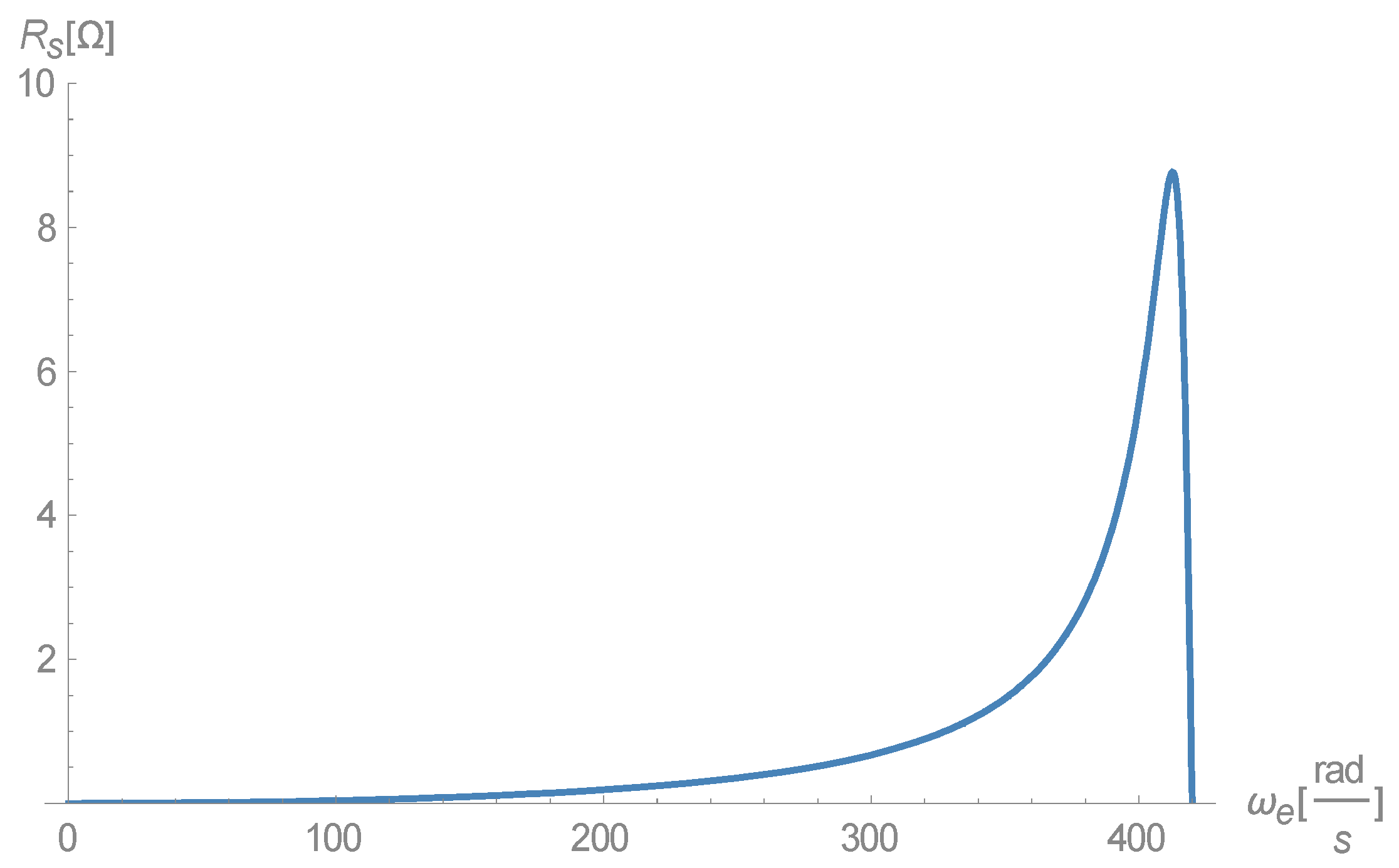
The substitution of ${\mathrm{R}}_{\mathrm{r}}=3.9\mathsf{\Omega },{\mathsf{\omega }}_{\mathrm{r}}=420\frac{\mathrm{r}}{\mathrm{s}},{\mathrm{L}}_{\mathrm{r}}=0.52\mathrm{H},\mathrm{M}=0.3\mathrm{H}$ gives a result similar to the results described in a previous study [1]. The resulting ${\mathrm{R}}_{\mathrm{s}}\left({\mathsf{\omega }}_{\mathrm{e}}\right)$ graph is similar, and is given in Figure 2.

However, this is not exactly the same graph. The difference between the results obtained in the previous study [1] and the current offered ${\mathrm{R}}_{\mathrm{s}}\left({\mathsf{\omega }}_{\mathrm{e}}\right)$ function is, analytically:

$${\mathrm{R}}_{\mathrm{s}}\left({\mathsf{\omega }}_{\mathrm{e}}\right)-{\mathrm{R}}_{\mathrm{s}}^{\left[1\right]}\left({\mathsf{\omega }}_{\mathrm{e}}\right)=\frac{{\mathrm{M}}^2{\mathrm{R}}_{\mathrm{r}}{}^3{\mathsf{\omega }}_{\mathrm{e}}}{4{\mathrm{L}}_{\mathrm{r}}{}^2\left({\mathsf{\omega }}_{\mathrm{e}}+{\mathsf{\omega }}_{\mathrm{r}}\right)({\mathrm{R}}_{\mathrm{r}}{}^2+{\mathrm{L}}_{\mathrm{r}}{}^2{\left({\mathsf{\omega }}_{\mathrm{e}}+{\mathsf{\omega }}_{\mathrm{r}}\right)}^2)}$$

(30)

A plot of the difference between the two graphs shows it to be almost insignificant at these values, as shown in Figure 3.

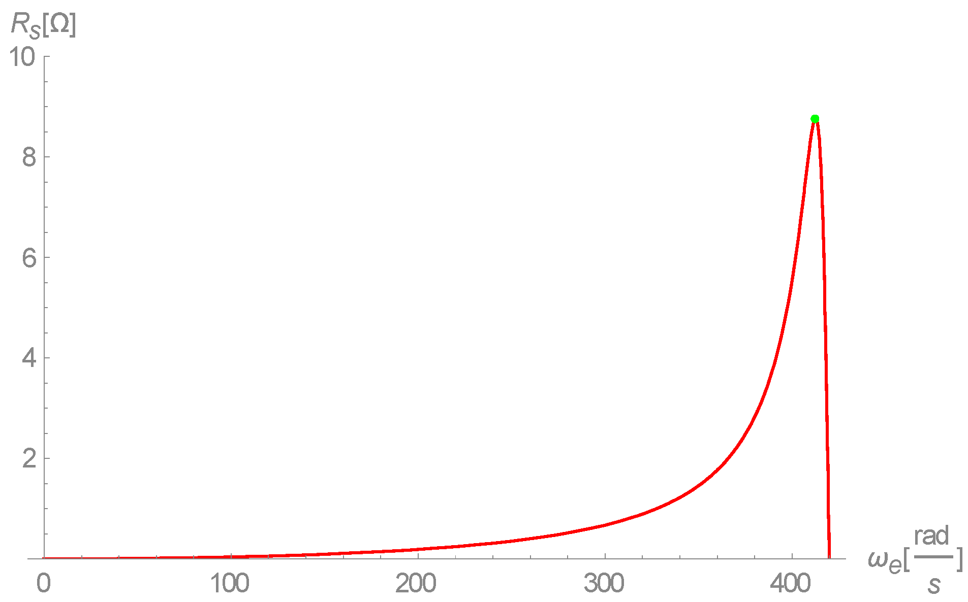
This difference could be more significant with other values. In any case, every value of ${\mathrm{R}}_{\mathrm{s}}$ fits to two-field frequencies, the higher of which is in the stable region of the generator. Currently, research interest lies in finding an analytical formula for the single frequency at which ${\mathrm{R}}_{\mathrm{s}}$ is maximal, ${\mathsf{\omega }}_{{\mathrm{e}}_{{\mathrm{R}}_{{\mathrm{s}}_{\max }}}}$. This formula can be easily obtained from Equation (29). Derivation and equating to zero gives five solutions, only one of which fits the physical mode of the machine.

$$\begin{array}{cc}\hfill \{\left\{{\mathsf{\omega }}_{\mathrm{e}}\to 0\right\},\{{\mathsf{\omega }}_{\mathrm{e}}& \to -\frac{\sqrt{-{\mathrm{R}}_{\mathrm{r}}{}^3+{\mathrm{L}}_{\mathrm{r}}{\mathrm{R}}_{\mathrm{r}}{}^2{\mathsf{\omega }}_{\mathrm{r}}-{\mathrm{L}}_{\mathrm{r}}{}^2{\mathrm{R}}_{\mathrm{r}}{\mathsf{\omega }}_{\mathrm{r}}{}^2+{\mathrm{L}}_{\mathrm{r}}{}^3{\mathsf{\omega }}_{\mathrm{r}}{}^3}}{\sqrt{{\mathrm{L}}_{\mathrm{r}}{}^2{\mathrm{R}}_{\mathrm{r}}+{\mathrm{L}}_{\mathrm{r}}{}^3{\mathsf{\omega }}_{\mathrm{r}}}}\},\{\mathsf{\omega }\mathrm{e}\hfill \\ & \to \frac{\sqrt{-{\mathrm{R}}_{\mathrm{r}}{}^3+{\mathrm{L}}_{\mathrm{r}}{\mathrm{R}}_{\mathrm{r}}{}^2{\mathsf{\omega }}_{\mathrm{r}}-{\mathrm{L}}_{\mathrm{r}}{}^2{\mathrm{R}}_{\mathrm{r}}{\mathsf{\omega }}_{\mathrm{r}}{}^2+{\mathrm{L}}_{\mathrm{r}}{}^3{\mathsf{\omega }}_{\mathrm{r}}{}^3}}{\sqrt{{\mathrm{Lr}}^2\mathrm{Rr}+{\mathrm{Lr}}^3{\mathsf{\omega }}_{\mathrm{r}}}}\},\{\mathsf{\omega }\mathrm{e}\hfill \\ & \to -\frac{\sqrt{{\mathrm{R}}_{\mathrm{r}}{}^3+{\mathrm{L}}_{\mathrm{r}}{\mathrm{R}}_{\mathrm{r}}{}^2{\mathsf{\omega }}_{\mathrm{r}}+{\mathrm{L}}_{\mathrm{r}}{}^2{\mathrm{R}}_{\mathrm{r}}{\mathsf{\omega }}_{\mathrm{r}}{}^2+{\mathrm{L}}_{\mathrm{r}}{}^3{\mathsf{\omega }}_{\mathrm{r}}{}^3}}{\sqrt{-{\mathrm{L}}_{\mathrm{r}}{}^2{\mathrm{R}}_{\mathrm{r}}+{\mathrm{L}}_{\mathrm{r}}{}^3{\mathsf{\omega }}_{\mathrm{r}}}}\},\{\mathsf{\omega }\mathrm{e}\hfill \\ & \to \frac{\sqrt{{\mathrm{R}}_{\mathrm{r}}{}^3+{\mathrm{L}}_{\mathrm{r}}{\mathrm{R}}_{\mathrm{r}}{}^2{\mathsf{\omega }}_{\mathrm{r}}+{\mathrm{L}}_{\mathrm{r}}{}^2{\mathrm{R}}_{\mathrm{r}}{\mathsf{\omega }}_{\mathrm{r}}{}^2+{\mathrm{L}}_{\mathrm{r}}{}^3{\mathsf{\omega }}_{\mathrm{r}}{}^3}}{\sqrt{-{\mathrm{L}}_{\mathrm{r}}{}^2{\mathrm{R}}_{\mathrm{r}}+{\mathrm{L}}_{\mathrm{r}}{}^3{\mathsf{\omega }}_{\mathrm{r}}}}\}\}\hfill \end{array}$$

(31)

The negative solutions are not physical, nor is zero a valid solution. This leaves two solutions for ${\mathsf{\omega }}_{{\mathrm{e}}_{{\mathrm{R}}_{{\mathrm{s}}_{\max }}}}$: $\frac{\sqrt{-{\mathrm{R}}_{\mathrm{r}}{}^3+{\mathrm{L}}_{\mathrm{r}}{\mathrm{R}}_{\mathrm{r}}{}^2{\mathsf{\omega }}_{\mathrm{r}}-{\mathrm{L}}_{\mathrm{r}}{}^2{\mathrm{R}}_{\mathrm{r}}{\mathsf{\omega }}_{\mathrm{r}}{}^2+{\mathrm{L}}_{\mathrm{r}}{}^3{\mathsf{\omega }}_{\mathrm{r}}{}^3}}{\sqrt{{\mathrm{L}}_{\mathrm{r}}{}^2{\mathrm{R}}_{\mathrm{r}}+{\mathrm{L}}_{\mathrm{r}}{}^3{\mathsf{\omega }}_{\mathrm{r}}}}$ and $\frac{\sqrt{{\mathrm{R}}_{\mathrm{r}}{}^3+{\mathrm{L}}_{\mathrm{r}}{\mathrm{R}}_{\mathrm{r}}{}^2{\mathsf{\omega }}_{\mathrm{r}}+{\mathrm{L}}_{\mathrm{r}}{}^2{\mathrm{R}}_{\mathrm{r}}{\mathsf{\omega }}_{\mathrm{r}}{}^2+{\mathrm{L}}_{\mathrm{r}}{}^3{\mathsf{\omega }}_{\mathrm{r}}{}^3}}{\sqrt{-{\mathrm{L}}_{\mathrm{r}}{}^2{\mathrm{R}}_{\mathrm{r}}+{\mathrm{L}}_{\mathrm{r}}{}^3{\mathsf{\omega }}_{\mathrm{r}}}}$.

However, the solution with the smaller denominator gives a frequency which is higher than that of the rotor. In short, it describes the machine working as a motor, but not as a generator. For example, with the parameters as before:

$$\frac{\sqrt{{\mathrm{R}}_{\mathrm{r}}{}^3+{\mathrm{L}}_{\mathrm{r}}{\mathrm{R}}_{\mathrm{r}}{}^2{\mathsf{\omega }}_{\mathrm{r}}+{\mathrm{L}}_{\mathrm{r}}{}^2{\mathrm{R}}_{\mathrm{r}}{\mathsf{\omega }}_{\mathrm{r}}{}^2+{\mathrm{L}}_{\mathrm{r}}{}^3{\mathsf{\omega }}_{\mathrm{r}}{}^3}}{\sqrt{-{\mathrm{L}}_{\mathrm{r}}{}^2{\mathrm{R}}_{\mathrm{r}}+{\mathrm{L}}_{\mathrm{r}}{}^3{\mathsf{\omega }}_{\mathrm{r}}}}=427.636\frac{\mathrm{rad}}{\mathrm{s}}.$$

Therefore, the only physical solution is:

$${\mathsf{\omega }}_{{\mathrm{e}}_{{\mathrm{R}}_{{\mathrm{s}}_{\max }}}}=\frac{\sqrt{-{\mathrm{R}}_{\mathrm{r}}{}^3+{\mathrm{L}}_{\mathrm{r}}{\mathrm{R}}_{\mathrm{r}}{}^2{\mathsf{\omega }}_{\mathrm{r}}-{\mathrm{L}}_{\mathrm{r}}{}^2{\mathrm{R}}_{\mathrm{r}}{\mathsf{\omega }}_{\mathrm{r}}{}^2+{\mathrm{L}}_{\mathrm{r}}{}^3{\mathsf{\omega }}_{\mathrm{r}}{}^3}}{\sqrt{{\mathrm{L}}_{\mathrm{r}}{}^2{\mathrm{R}}_{\mathrm{r}}+{\mathrm{L}}_{\mathrm{r}}{}^3{\mathsf{\omega }}_{\mathrm{r}}}}$$

(32)

Maintaining parameters as before, this would yield ${\mathsf{\omega }}_{{\mathrm{e}}_{{\mathrm{R}}_{{\mathrm{s}}_{\max }}}}=412.632\frac{\mathrm{rad}}{\mathrm{s}}$.

Substitution of Equation (32) into Equation (29) results in:

$${\mathrm{R}}_{{\mathrm{s}}_{\max }}=\frac{{\mathrm{M}}^2{\left({\mathrm{R}}_{\mathrm{r}}-{\mathrm{L}}_{\mathrm{r}}{\mathsf{\omega }}_{\mathrm{r}}\right)}^2}{8{\mathrm{L}}_{\mathrm{r}}{}^3{\mathsf{\omega }}_{\mathrm{r}}}$$

(33)

which is an improvement to the equation in Reference [1] (${\mathrm{R}}_{{\mathrm{s}}_{\max }}=\frac{{\mathrm{M}}^2}{8{\mathrm{L}}_{\mathrm{r}}}\cdot {\mathsf{\omega }}_{{\mathrm{e}}_{{\mathrm{R}}_{{\mathrm{s}}_{\max }}}}$). Practically, with the parameters designated as in a previous study [1], the approximation from this study yields ${\mathrm{R}}_{{\mathrm{s}}_{\max }}=8.7649\mathsf{\Omega }$, while by the previous approximations [1], the value would be $8.927\mathsf{\Omega }$. Therefore, the machine would cease to operate as a generator for a slightly lower value using the current approximation than previous results suggest [1]. Combining the last results to obtain the curve in Figure 4:

This result is more accurate than that given in Reference [1], where it was approximated as:

$${\mathsf{\omega }}_{{\mathrm{e}}_{{\mathrm{R}}_{{\mathrm{s}}_{{\max }_2}}}}={\mathsf{\omega }}_{\mathrm{r}}-\frac{{\mathrm{R}}_{\mathrm{r}}}{{\mathrm{L}}_{\mathrm{r}}}=412.5\frac{\mathrm{rad}}{\mathrm{s}}$$

4. Numerical Analysis on the Stator Current Frequency

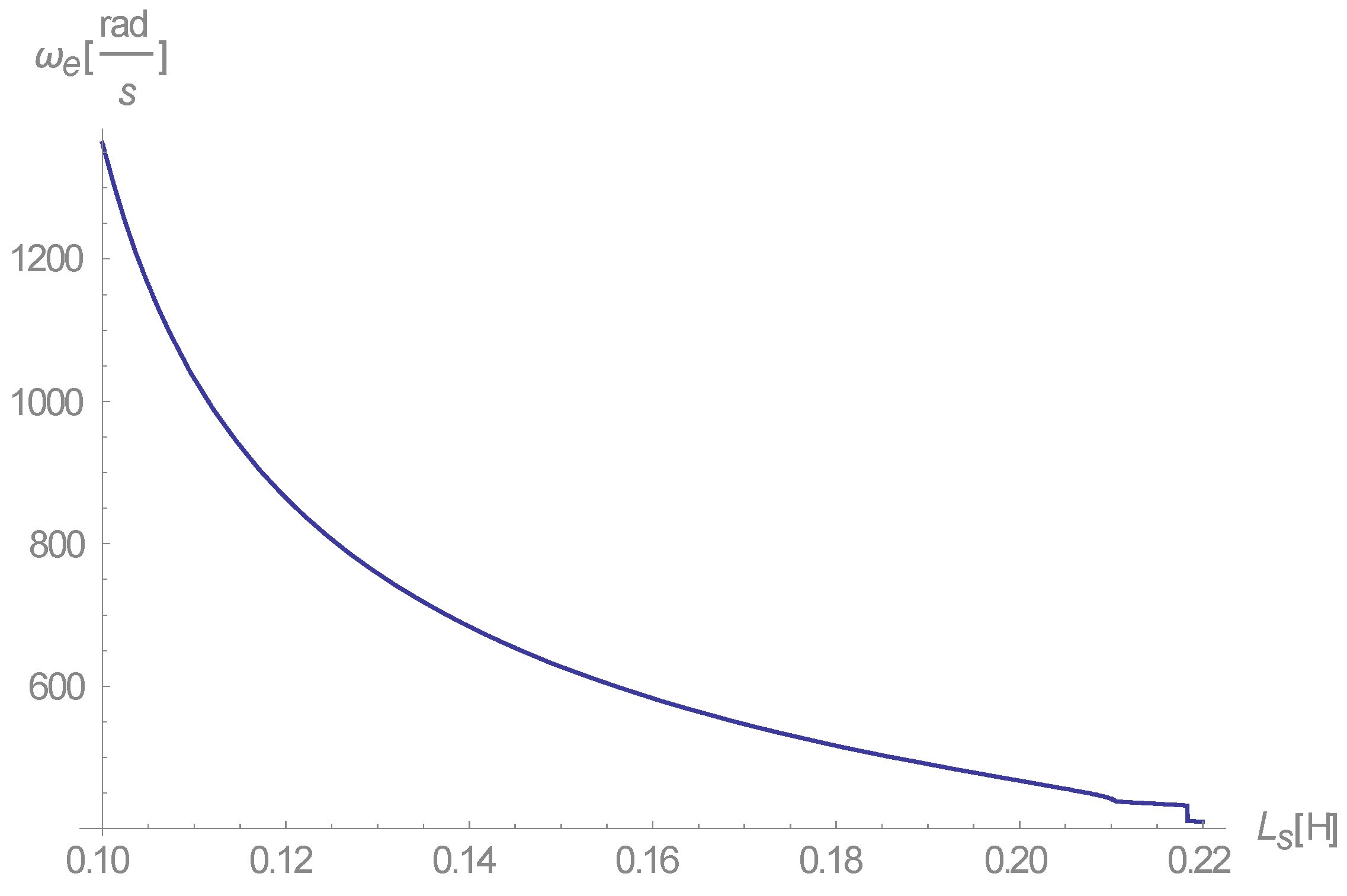
The exploration of Equation (27), $\frac{1}{{\mathrm{c}\mathsf{\omega }}_{\mathrm{e}}}+\frac{{\mathrm{M}}^2{\mathsf{\omega }}_{\mathrm{e}}\left({\mathrm{L}}_{\mathrm{r}}\left({\mathrm{L}}_{\mathrm{r}}{\mathrm{r}}^2{\left({\mathsf{\omega }}_{\mathrm{e}}{}^2-{\mathsf{\omega }}_{\mathrm{r}}{}^2\right)}^2\right)\right)}{2({\mathrm{Lr}}^2{\left({\mathsf{\omega }}_{\mathrm{e}}-{\mathsf{\omega }}_{\mathrm{r}}\right)}^2+{\mathrm{R}}_{\mathrm{r}}{}^2)({\mathrm{L}}_{\mathrm{r}}{}^2{\left({\mathsf{\omega }}_{\mathrm{e}}+{\mathsf{\omega }}_{\mathrm{r}}\right)}^2+{\mathrm{R}}_{\mathrm{r}}{}^2)}-{\mathrm{L}}_{\mathrm{s}}{\mathsf{\omega }}_{\mathrm{e}}=0$, is more difficult than that of Equation (29). The aim here, as in previous analyses [1], is to deduce the limits of ${\mathsf{\omega }}_{\mathrm{e}}$. Therefore, a solution for Equation (27) for ${\mathsf{\omega }}_{\mathrm{e}}$ is required. This solution yields six huge multi-term solutions in positive/negative pairs, which can only be explored numerically under the same parameters as before. For example, using previous parameters, a plot of the imaginary part of the first solution of ${\mathsf{\omega }}_{\mathrm{e}}$ (L_S) yields the curve depicted in Figure 5.

This is simply not interesting, as with a zero or positive imaginary part, this solution is evanescent, and does not deliver a stable solution. Thus, the first solution does not satisfy our requirements.

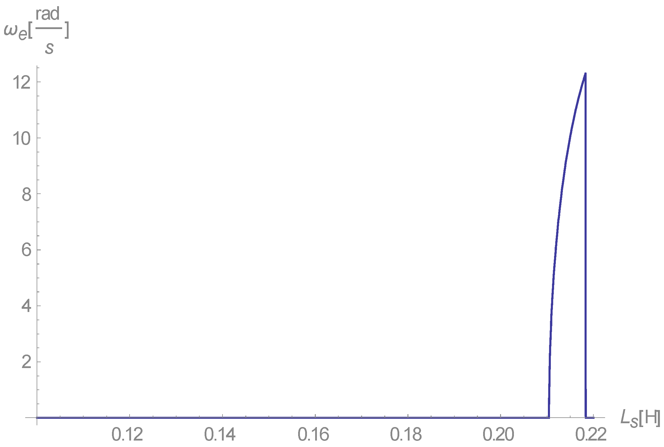
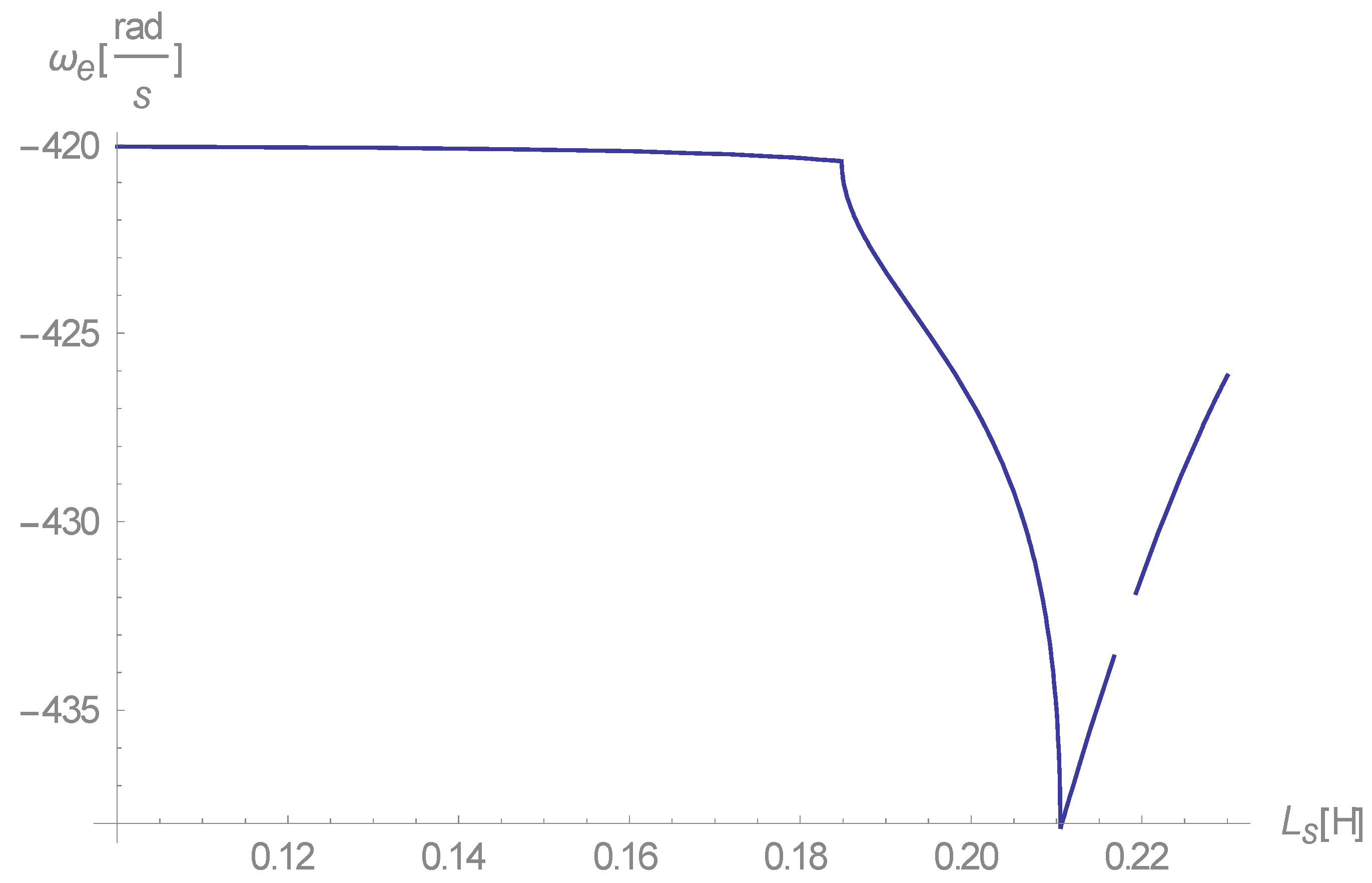
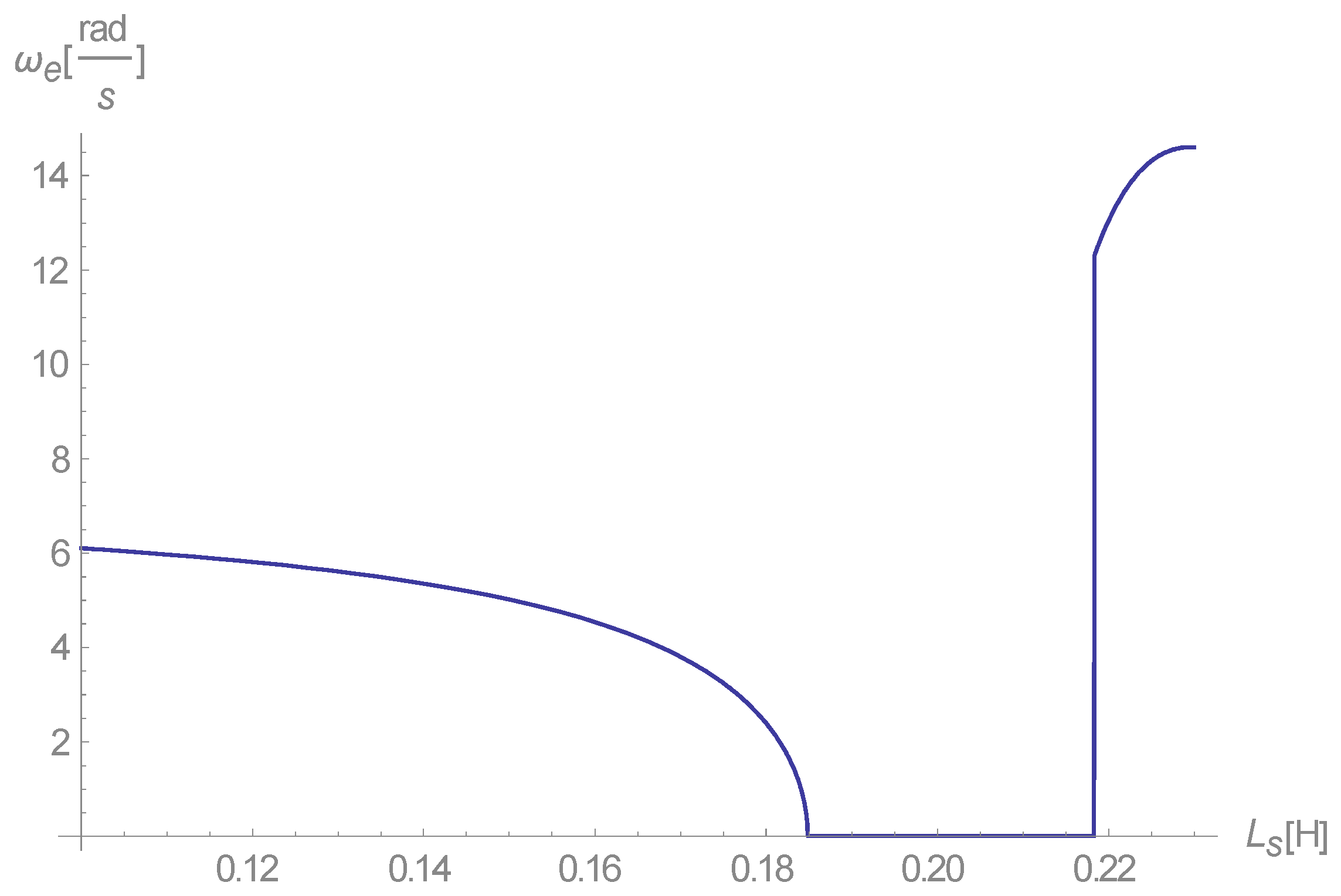
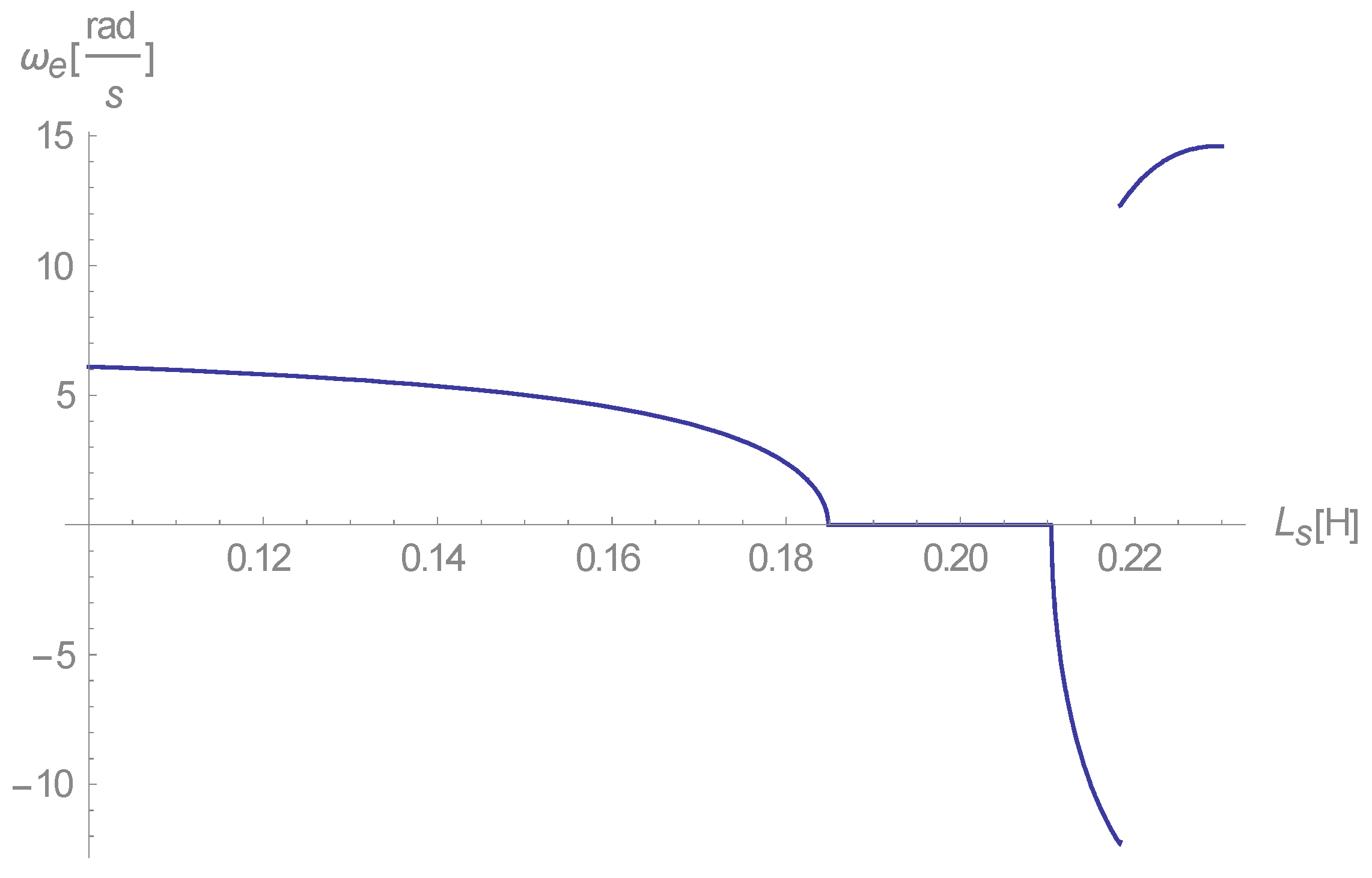
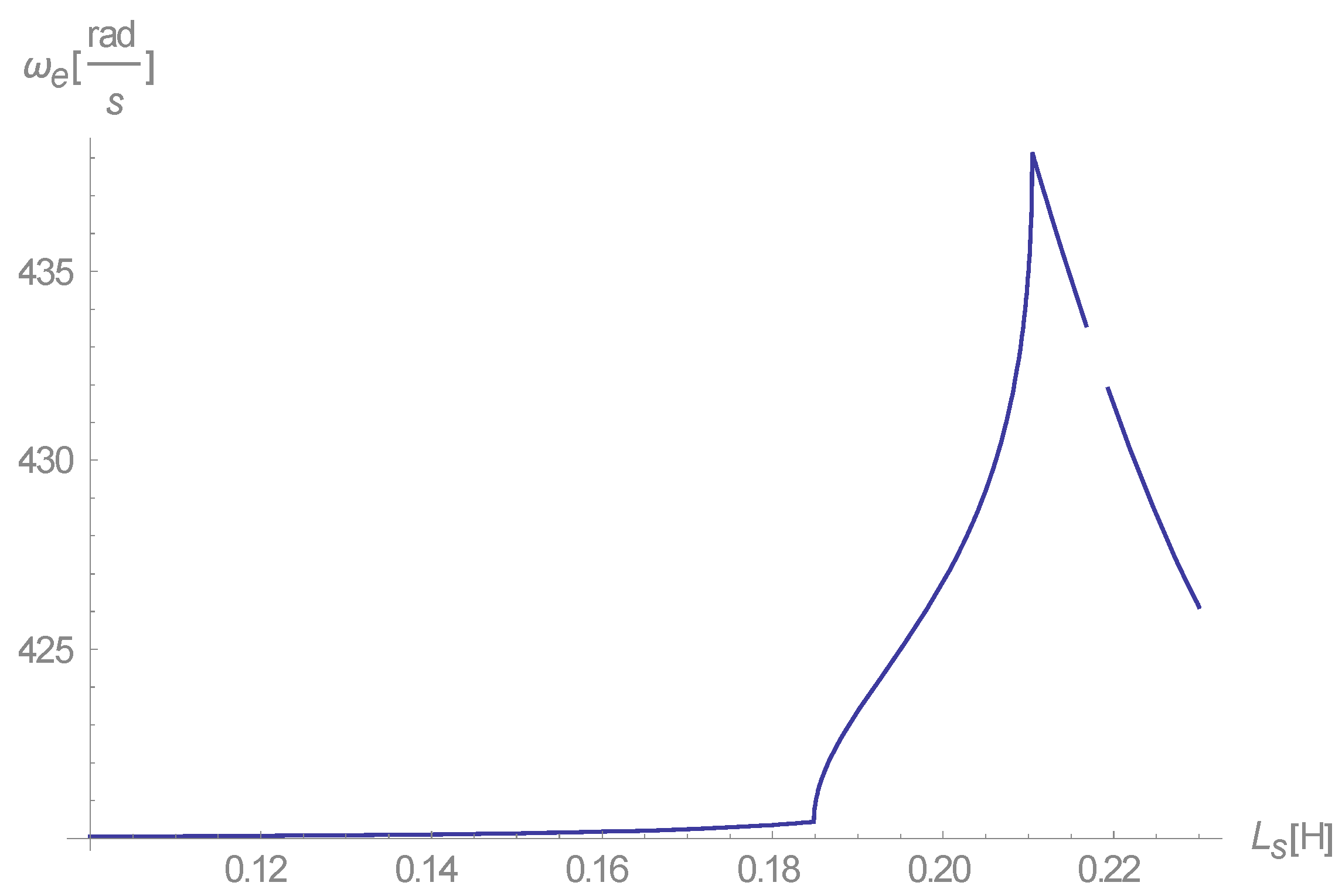
The second solution is more interesting, as its real part is depicted in Figure 6:

Overall, this curve (Figure 6) is a description of a motor. At Ls = ~0.22 H, there is a dip to a stable generator mode, which becomes evident when viewing the imaginary part (Figure 7).

The results shown in Figure 6 and Figure 7, which correspond to the second solution, represent the first solution that implies a stable generator mode.

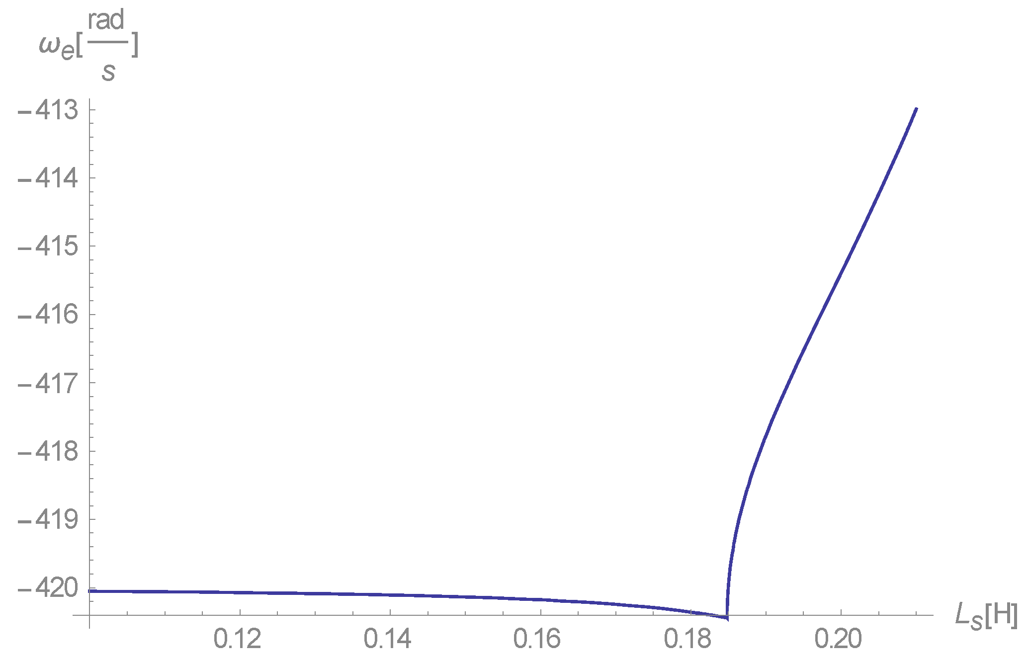
Solutions three and four are a positive-negative pair, as solution three has a real negative rotation (Figure 8), and only a small interval of a negative imaginary part, as shown in Figure 9.

However, the negative rotation strongly implies that this solution describes the action mode as a brake, rather than as a generator. Solution four fails to meet our requirements, as, similar to the first solution, its real part is demonstrated by the curve in Figure 10.

Figure 10 depicts a motor, not a generator, as its stator current rotation speed is higher than the physical speed of the rotor (420 rad/s). Solutions five and six are, again, a positive-negative pair. Solution five gives real negative speed, making it uninteresting in the scope of the IG. Its real part is demonstrated in Figure 11. Solution six is not interesting either, as its imaginary part, using the same parameters, produces the curve shown in Figure 12.

This solution has only a positive imaginary part, making it evanescent. Additionally, its imaginary part between ${\mathrm{L}}_{\mathrm{s}}\approx 0.185\mathrm{H}$ to ${\mathrm{L}}_{\mathrm{s}}\approx 0.215\mathrm{H}$ is zero, and as such no fluctuations at all are predicted by it in this range.

In short, solution two best describes a stable IG. However, the conclusion is that ${\mathrm{L}}_{\mathrm{s}}$ is highly limited to the range above 0.21 H, maintaining the previously outlined parameters [1].

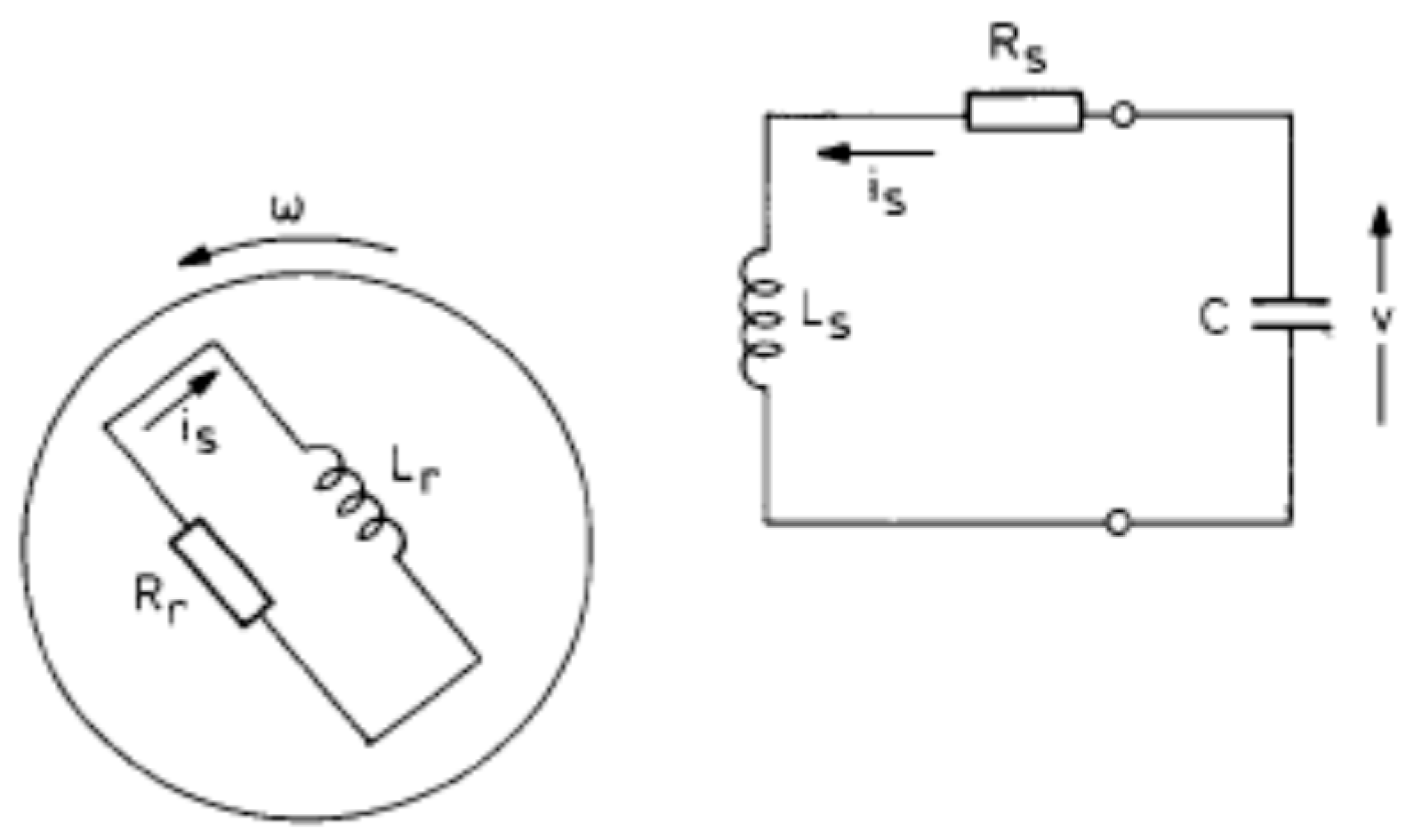
5. Computer Simulation of a Single-Phase Rotor, Single-Phase IG

It remains to be shown that the current in the rotor has a frequency that is twice the frequency of the stator. Since this is an asymmetrical machine and therefore reacts not unlike a Variable Reluctance Machine (VRM)—and unless ${\mathrm{L}}_{\mathrm{s}}>~0.21 \mathrm{H}$—the IG is not stable.

To prove this, a computer simulation of the machine was constructed using MATLAB based on Equations (1)–(3), which were solved using ode45. The resulting wave form was also pumped through FFT (Fast Fourier Transform) to obtain the frequency of the rotor. As this is a numerical simulation of the system of differential equations, it is devoid of approximations, enabling the validation of earlier approximations through deduction.

In this computer simulation, the core saturation was not taken into account. Therefore, the IG is stable when the simulation is exploding to infinity. This is valid since, as the stator currents grow, eventually the core is saturated and this makes them stabilize [7].

The simulation parameters, simulating a system with some losses, are identical to the machine parameters outlined previously [1]: a TERCO 1.5 kW Model MV-121 Slip Rings Induction Machine (Terco, Stockholm, Kungens Kurva industrial park, Sweden),

• L_s = 0.22
• L_r = 2.36·L_s~0.52 H
• R_r = 3.9
• R_s = 5.4
• ω_r = 420
• M = 1.38·L_s~0.3 H
• c = 4.1 × 10⁻⁵

As expected, the result with L_s = 0.22, indicates that a stable IG would be obtained. It should be clear in this context that the magnetic saturation of the machine is not modeled here. A stable run of the machine has been previously conducted [1]. A simulation without magnetic saturation yields Figure 13:

With L_s = 0.18 H the result is demonstrated in Figure 14:

Where L_s = 0.2 H, as this is almost at the boundary, the result is more interesting and is shown in Figure 15:

Therefore, it is demonstrated that for ${\mathrm{L}}_{\mathrm{s}}<~0.21 \mathrm{H}$, the IG is not stable.

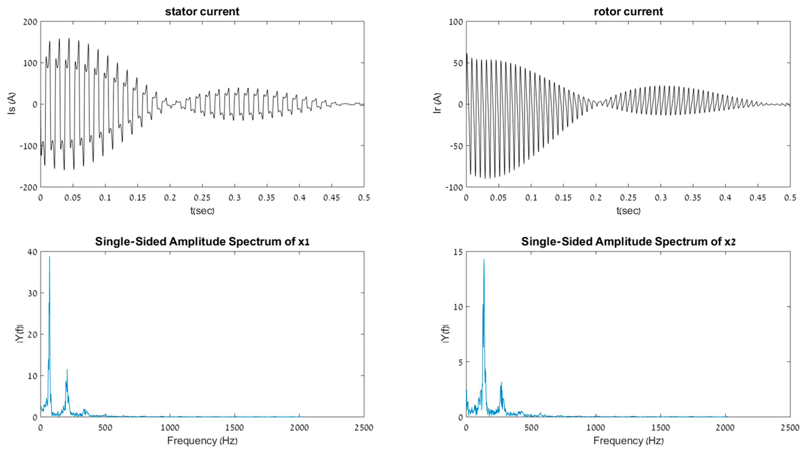
It remains to be seen that the rotor current frequency basic harmonics is at twice the stator current. This can be easily shown by plotting the rotor current as well, and pumping both through FFT. The results are given in Figure 16:

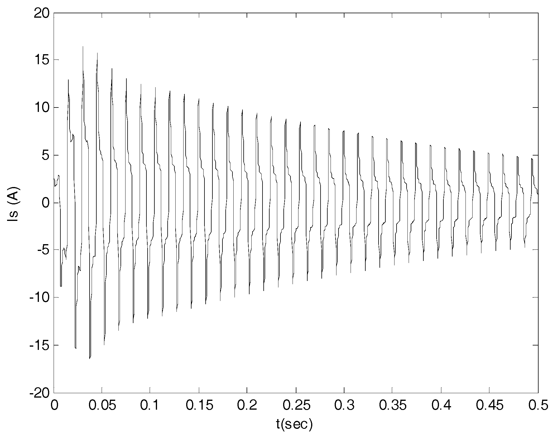
At the boundary, ${\mathrm{L}}_{\mathrm{s}}=0.21\mathrm{H}$ exactly, the IG is marginally stable, as evidenced by the simulation when run for 0.5 s (Figure 17).

At this point, the stability of the machine is highly dependent on the value of Rs. For example, increasing its value above Rs_max would yield an evanescent response. Figure 18 shows the simulation response if ${\mathrm{L}}_{\mathrm{s}}=0.21\mathrm{H},{\mathrm{R}}_{\mathrm{s}}=9\mathsf{\Omega }$, which is slightly above Rs_max.

6. Conclusions

A model for an IG was explored with in-depth investigation into first harmonics of the mutual inductance effect on the machine. Additionally, the resulting solutions for the stator field’s angular frequency as a limiting factor for the stability of the IG were studied.

An improved exact equation for the maximum allowable resistivity of the stator circuit, allowing stable operation as a single-phase stator, single-phase rotor machine was reached. In addition, the frequency of the stator current in such a mode was determined.

A simulation of the IG was then run, verifying the approximations done in exploration of the IG model. It was shown that the rotor current frequency is twice that of the stator current, and the stability region of the IG coincides with the theoretical analysis. On the boundary, the value of the resistivity of the stator circuit model was validated as well.

Practical uses of this work could involve the use of any of the physical solutions found in Section 4. These uses may include new types of machines, working as a single-phase brake, generator, or motor, in a multiple-phase system. However, this exceeds the scope of this article, and as such is left for future research.