Optimizing the District Heating Primary Network from the Perspective of Economic-Specific Pressure Loss

Abstract
1. Introduction
2. Methods
2.1. Calculate the Mass Flow Rate in Each Pipe
2.2. Determine the Possible Combinations of Diameters for the Pipes
- The diameters of upstream pipes are larger or equal to the consecutive downstream pipes in the main supply line, and the order is reversed in the main return line;
- The main supply and return lines are symmetrical.
2.3. Calculate the Water Flow Velocity, Pressure Loss ∆P in Each Pipe, and Specific Pressure Loss R
2.4. Sort the Pipe Combination Scenarios According to R
2.5. Calculate the Initial Investment for Each Network Scenario Using the Variable Prices of Insulated District Heating Pipes
2.6. Determine the Lift Head and Equivalent Full Operating Time of the Pump Using a Variable, Full Operating Percentage for the Year
2.7. Calculate the Pump Power and Electric Motor Power
2.8. Calculate the Electricity Consumption, Pumping Cost, Heat Loss, and Heat Distribution Cost for Different Network Scenarios
2.9. Calculate the Annuity on the Initial Investment and the Total Annual Cost
2.10. Show the Optimization Results
3. Results and Discussion
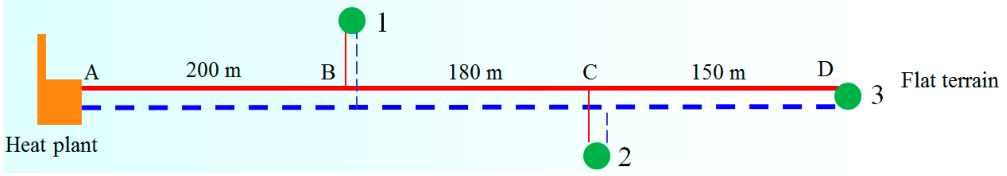
3.1. The DH Network Used in the Case Study
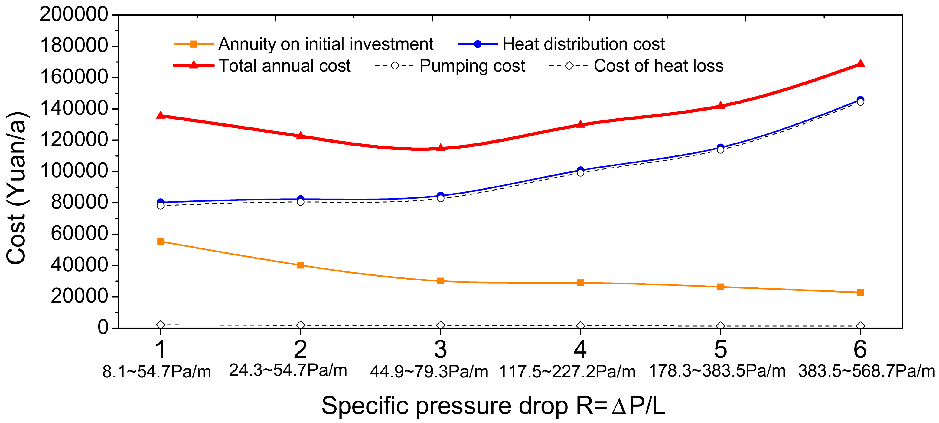
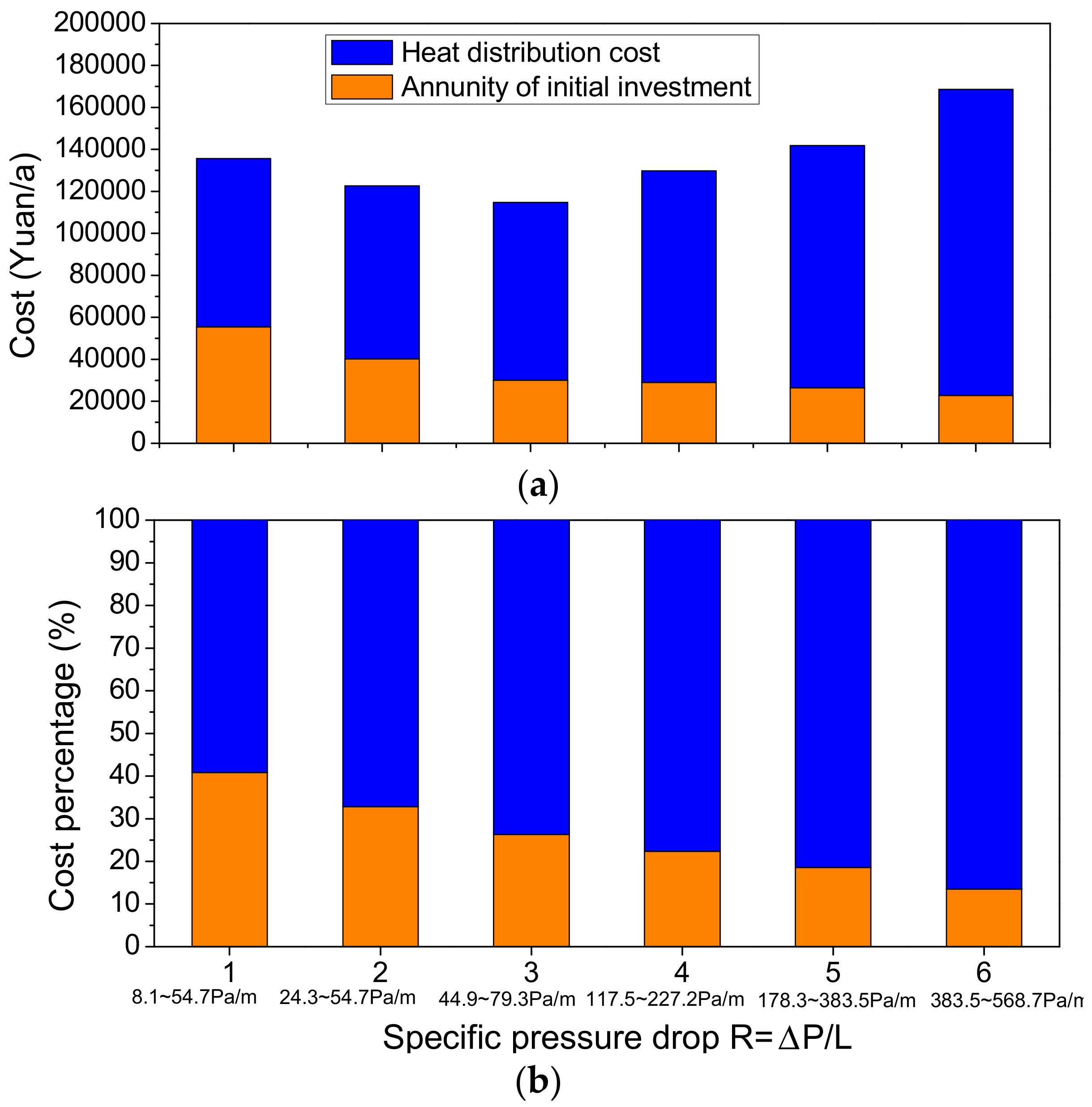
3.2. Optimization Results
3.3. Discussion
4. Conclusions
Acknowledgments
Author Contributions
Conflicts of Interest
References
- Finnish Energy Industries. Energy Year 2013—District Heat. Available online: http://energia.fi/en/statistics-and-publications (accessed on 7 April 2017).
- Wang, H.C.; Jiao, W.L.; Zou, P.H.; Liu, J.C. Analysis of an effective solution to excessive heat supply in a city primary heating network using gas-fired boilers for peak-load compensation. Energy Build. 2010, 42, 2090–2097. [Google Scholar] [CrossRef]
- Wang, H.C.; Jiao, W.L.; Lahdelma, R.; Zou, P.H. Techno-economic analysis of a coal-fired CHP based combined heating system with gas-fired boilers for peak load compensation. Energy Policy 2011, 39, 7950–7962. [Google Scholar]
- Calì, M.; Borchiellini, R. District heating networks calculation and optimization. In Exergy, Energy System Analysis, and Optimization; EOLSS: Paris, France, 2013; Volume 2. [Google Scholar]
- Ministry of Housing and Urban-Rural Development of the People’s Republic of China. Design Code for City Heating Network (CJJ34-2010); Achitecture & Building Press: Beijing, China, 2010.
- Frederiksen, S.; Wener, S. District Heating and Cooling; Studentlitteratur: Lund, Sweden, 2013. [Google Scholar]
- Lahdelma, R.; Wang, H.C. District Heating Distribution, 2nd International DHC + Summer School Course, a Bridge towards Future Energy System; Aalto University: Helsinki, Finland, 2014. [Google Scholar]
- Jiang, Y.; Yang, X. Current status of building energy consumption in China and problems in building energy saving. China Constr. 2006, 2, 12–18. [Google Scholar]
- Jiang, Y. Measures to Increase the Energy Efficiency of District Heating Energy Sources; Building Energy Saving Research Center of Tsinghua University: Beijing, China, 2014. [Google Scholar]
- Wang, C.Q.; Wang, S.Z.; Xu, K.; Cao, D.D.; Wang, Y.F.; Bai, L.; Dai, X. Heat loss measurement anlaysis of central heating pipe network. J. Jinlin Jianzhu Univ. 2015, 32, 39–41. [Google Scholar]
- Vesterlund, M.; Sandberg, J.; Lindblom, B.; Dahl, J. Evaluation of losses in district heating syste, a case study. In Proceedings of the International Conference on Efficiency, Cost, Optimization, Simulation & Environmental Impact of Energy Systems, Guilin, China, 16–19 July 2013. [Google Scholar]
- Çomaklı, K.; Yüksel, B.; Çomaklı, Ö. Evaluation of energy and energy losses in district heating network. Appl. Therm. Eng. 2004, 24, 1009–1017. [Google Scholar] [CrossRef]
- Mertz, T.; Serra, S.; Henon, A.; Reneaume, J. A MINLP optimization of the configuration and the design of a district heating network: Academic study cases. Energy 2016, 117, 450–464. [Google Scholar]
- Morvaj, B.; Evins, R.; Carmeliet, J. Optimising urban energy systems: Simultaneous system sizing, operation and district heating network layout. Energy 2016, 116, 619–636. [Google Scholar]
- Haikarainen, C.; Pettersson, F.; Saxén, H. A model for structural and operational optimization of distributed energy systems. Appl. Therm. Eng. 2014, 70, 211–218. [Google Scholar]
- Hassine, I.B.; Eicker, U. Impact of load structure variation and solar thermalenergy integration on an existing district heating network. Appl. Therm. Eng. 2013, 50, 1437–1446. [Google Scholar]
- Wang, W.H.; Cheng, X.T.; Liang, X.G. Optimization modeling of district heating networks and calculation by the Newton method. Appl. Therm. Eng. 2013, 61, 163–170. [Google Scholar]
- Zeng, J.; Han, J.; Zhang, G. Diameter optimization of district heating and cooling piping network based on hourly load. Appl. Therm. Eng. 2016, 107, 750–757. [Google Scholar] [CrossRef]
- Tol, H.I.; Svendsen, S. Improving the dimensioning of piping networks and network layouts in low-energy district heating systems connected to low-energy buildings: A case study in Roskilde, Denmark. Energy 2012, 38, 276–290. [Google Scholar] [CrossRef]
- Pirouti, M.; Bagdanavicius, A.; Ekanayake, J.; Wu, J.; Jenkins, N. Energy consumption and economic analyses of a district heating network. Energy 2013, 57, 149–159. [Google Scholar] [CrossRef]
- Koiv, T.A.; Mikola, A.; Palmiste, U. The new dimensioning method of the district heating network. Appl. Therm. Eng. 2014, 71, 78–82. [Google Scholar] [CrossRef]
- Ancona, M.A.; Melino, F.; Peretto, A. An Optimization procedure for District Heating networks. Energy Procedia 2014, 61, 278–281. [Google Scholar] [CrossRef]
- Jie, P.; Kong, X.; Rong, X.; Xie, S. Selecting the optimum pressure drop per unit length of district heating piping network based on operating strategies. Appl. Energy 2016, 177, 341–353. [Google Scholar] [CrossRef]
- Rezaie, B.; Rosen, M.A. District heating and cooling: Review of technology and potential enhancements. Appl. Energy 2012, 93, 2–10. [Google Scholar] [CrossRef]
- Mavrotas, G.; Figueira, J.R.; Siskos, E. Robustness analysis methodology for multi-objective combinatorial optimization problems and application to project selection. Omega 2015, 52, 142–155. [Google Scholar] [CrossRef]
- Larsen, H.V.; Pálsson, H.; Bøhm, B.; Ravn, H.F. Aggregated dynamic simulation model of district heating networks. Energy Convers. Manag. 2002, 43, 995–1019. [Google Scholar] [CrossRef]
- Larsen, H.V.; Bøhm, B.; Wigbels, M. A comparison of aggregated models for simulation and operational optimisation of district heating networks. Energy Convers. Manag. 2004, 45, 1119–1139. [Google Scholar] [CrossRef]
- National Standard of the People’s Republic of China. Design Code for Heating Ventilation and Air Conditioning of Civil Buildings; China Architecture & Building Press: Beijing, China, 2012.
- He, P.; Sun, G.; Wang, F.; Wu, H.X. District Heating Engineering, 4th ed.; Architecture & Building Press: Beijing, China, 2009. [Google Scholar]
- Fang, T.; Lahdelma, R. State estimation of district heating network based on customer measurements. Appl. Therm. Eng. 2014, 73, 1211–1221. [Google Scholar] [CrossRef]
- Zhang, H.; Xi, J.; Guo, H. Calculation and analysis of heat loss and temperature drop along directly buried hot water heating pipeline. Gas Heat 2014, 34, A36–A38. [Google Scholar]
- Terhan, M.; Comakli, K. Energy and exergy analyses of natural gas-fired boilers in a district heating system. Appl. Therm. Eng. 2017, 121, 380–387. [Google Scholar] [CrossRef]


| Heat User No. | 1 | 2 | 3 |
|---|---|---|---|
| Heat demand (GJ/h) | 3.518 | 2.513 | 5.025 |
| Heat demand (kW) | 977 | 698 | 1396 |
| Parameter | Description |
|---|---|
| Heat season | 150 d |
| Pressure drop in the heat plant | 80 kPa |
| Static pressure | 40 mH2O (1 kPa ≈ 0.102 mH2O) 1 |
| Local resistance pressure loss rate | 30% |
| Interest rate | 7.56% |
| Heat price | 50 Yuan/GJ |
| Electricity price | 0.8 Yuan/kWh |
| Calculation period | 20 years |
| Pipe prices based on steel consumption | 360,000 (L); 420,000 (I); 480,000 (H) Yuan/m3 2 |
| Pump operating time percentage | 40% (L); 60% (I); 80% (H) of full power operating time 3 |
| Pump efficiency | 70% |
| Water density (average) | 958.4 kg/m3 |
| Inner surface roughness | 0.005 m |
| Assurance coefficient S | 1.15 |
| Efficiency of motor ηm | 80% |
| Scenario No. | 1 | 2 | 3 | 4 | 5 | 6 | |
|---|---|---|---|---|---|---|---|
| R = ∆P/L (Pa/m) 1 | 8.1~54.7 | 24.3~54.7 | 44.9~79.3 | 117.5~227.2 | 178.3~383.5 | 383.5~568.7 | |
| Pipe diameter (mm) 2 | A->B | 219 × 6 | 159 × 4.5 | 159 × 4.5 | 133 × 4 | 108 × 4 | 108 × 4 |
| B->C | 133 × 4 | 133 × 4 | 133 × 4 | 108 × 4 | 108 × 4 | 89 × 3.5 | |
| C->D | 133 × 4 | 133 × 4 | 108 × 4 | 89 × 3.5 | 89 × 3.5 | 76 × 3.5 | |
© 2017 by the authors. Licensee MDPI, Basel, Switzerland. This article is an open access article distributed under the terms and conditions of the Creative Commons Attribution (CC BY) license (http://creativecommons.org/licenses/by/4.0/).
Share and Cite
Wang, H.; Duanmu, L.; Li, X.; Lahdelma, R. Optimizing the District Heating Primary Network from the Perspective of Economic-Specific Pressure Loss. Energies 2017, 10, 1095. https://doi.org/10.3390/en10081095
Wang H, Duanmu L, Li X, Lahdelma R. Optimizing the District Heating Primary Network from the Perspective of Economic-Specific Pressure Loss. Energies. 2017; 10(8):1095. https://doi.org/10.3390/en10081095
Chicago/Turabian StyleWang, Haichao, Lin Duanmu, Xiangli Li, and Risto Lahdelma. 2017. "Optimizing the District Heating Primary Network from the Perspective of Economic-Specific Pressure Loss" Energies 10, no. 8: 1095. https://doi.org/10.3390/en10081095
APA StyleWang, H., Duanmu, L., Li, X., & Lahdelma, R. (2017). Optimizing the District Heating Primary Network from the Perspective of Economic-Specific Pressure Loss. Energies, 10(8), 1095. https://doi.org/10.3390/en10081095