Numerical Study on the Internal Flow Field of a Reversible Turbine during Continuous Guide Vane Closing

Abstract

The unsteady flow field in a reversible pump-turbine is investigated during the continuous load rejection using a 3D computational fluid dynamic analysis. Numerical calculations are carried out using the detached eddy simulation (DES) turbulence model and a new approach involving automatic mesh motion. In this way, the instability of the flow field is analyzed by continuously changing the guide vane openings from the best efficiency point (BEP). Unsteady flow characteristics are described by post-processing signals for several monitoring points including mass flow, torque, head and pressure in the frequency and time-frequency domains. The formation of vortices of different scales is observed from the origin to further enlargement and stabilization; the effect of the rotating structures on the flow passage is analyzed, and the influence of unsteady flow development on the performance of the turbine is investigated. Finally, the evolution during the period of load rejection is characterized in order to determine the hydrodynamic conditions causing the vibrations in the machine.

1. Introduction

In the last few decades, significant and unpredictable developments in the research of new energy sources have made electrical energy storage become a key issue. At present, large-scale energy storage technology mainly consists of two different systems, compressed air energy storage (CAES) and reversible pumped hydro energy storage (RPHES). However, CAES require large caissons and still depend on fossil fuels; as a consequence, CAES applications are restricted to a large extent. On the other hand, most consider the RPHES as the best solution to store electricity indirectly: pumping the water upstream allows storing potential energy in the pump condition; the position potential energy is therefore converted into kinetic energy under the turbine condition, and finally, electricity can be generated and sent to the grid. The presence of associated regulations allowed a still ongoing strong deployment of renewable energy sources (RENS) technologies; however, due to the unpredictable evolution of RENS, RPHES needs to balance the frequency changes in electricity production and consumption. The trend seems to indicate that RPHES is experiencing a sustainable development, as stated by Barbour et al. [1].

Reversible turbines are more popular compared to other forms of turbomachinery in the new generation of RPHES, due to the considerable cost effectiveness and high efficiency range. Furthermore, they gain a competitive advantage and have efficient switch connections between electricity production and consumption (Beevers et al. [2] and Fisher et al. [3]). A Reversible Pump Turbine (RPT) can deal with problems related to the conversion and input of energy into the grid, due to the need for switching between pump and turbine mode. However, during periods of changing conditions between pump and turbine modes, starting up and stopping of the unit and load rejection, there is the need to change the speed and high frequency to compensate the off-design conditions, as shown in the S-shaped characteristic curves. As a consequence, the unit performance, regulation capacity and efficiency are affected, and both cavitation and instability phenomena could appear. The change in load, together with frequent starts and stops, represents one of the most important characteristics of a pump-turbine: it allows one to counter the increased need for leveling the peak demand of electrical energy and to better balance the system. For these reasons, pump-turbines’ working conditions are particularly suitable to be investigated using unsteady analyses [4,5].

RPTs need to be quickly disconnected from the power system when load changes or unpredictable situations occur; in order to reduce the unit damage, caused by the sudden increment of rotating speed, the guide vane must be rapidly closed accordingly. In addition, pump-turbines are synchronized with the electrical grid during load rejection; however, the procedure could be slowed down by system oscillations caused by the unstable behavior: longer times greatly contribute to unit damage.

The oscillatory phenomena had been originally studied by Yamabe [6]: the pronounced hysteretic behavior of oscillations in the values of pressure was observed and its interaction with unsteady cavitation patterns analyzed. Several authors carried out an in-depth study of the unsteady flow phenomena: Klemm [7] gave a simple solution of the instability of the flow by detuning some guide vanes; Martin [8] made a linear stability analysis to predict the occurrence of the oscillations. Afterwards, Dörfler et al. [9] studied how stable operations on the machine could be achieved even in the presence of the instability at no load. In addition, several studies of Nicolet et al. in [10,11] investigated the severe problems of unstable behavior, which is induced by positive gradients of the pump turbine characteristic and also represented the time evolution of the damping for both the rigid and elastic water column modes. They finally demonstrated the higher instability of the elastic mode compared to the rigid mode. However, the above-mentioned analyses are not complete, and the requirements to limit the instability are not met: many RPHES also need to improve the stability in the period of rejecting and accepting load, in order to eliminate vibrations, to improve the S-curve characteristics and to cut down the surge pressure rises.

Recent studies have shown that the S-induced instabilities can be ascribed to flow phenomena, such as stationary vortex formation and rotating stall in the runner (Yin et al. [12], Zeng et al. [13] and Hasmatuchi et al. [14]). However, other aspects regarding unstable behavior in the load rejection phase should be further investigated: the onset and development of the vortices in the runner channels and the reasons for the further enlargement and stabilization. On the other hand, it is necessary to find the cause of vibration and propose effective control measures to reduce the instability phenomena in order to ensure the safety of the unit in a long-term operation. In order to illustrate the accuracy of the analysis, the test case adopted for the validation of the numerical model is represented by the pump-turbine of the Xiangshuijian pumped storage plant [15], and it has been widely studied by several authors [16,17,18]. However, the analyses of the unsteady phenomena in pump-turbines are not simple, and often experimental and numerical results differ; furthermore, the inner flow in the machine is difficult to investigate, and studies of unsteady processes have many limitations.

In previous works, a linear closing law has been applied to various power plants characterized by adverse flow field effects [19,20]. In fact, the suggested closing laws did not completely reduce the instabilities, and the flow field characteristics still need to be improved. On the other hand, several authors adopted some fixed guide vane positions in order to simulate the closing process, which cannot accurately reproduce the entire dynamic process [19,21].

In the present paper, 3D numerical simulations are used to investigate the off-design conditions of the reversible turbine, and an automatic moving mesh technique has been implemented in order to continuously assess the unsteady flow characteristics during guide vanes’ closure; the procedure also guarantees a high mesh quality during the whole process of load rejection. Furthermore, a new closing method consisting of five stages is given by combining the results of steady-state test data and unsteady simulations under fixed conditions. In fact, achieving stability of the unit under no-load condition is difficult using the existing closing laws; hence, the definition of an improved method is extremely important.

2. Model Geometry and Spatial Discretization

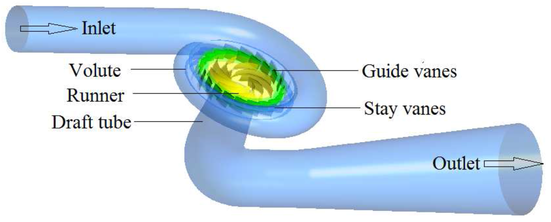
The geometric model of the considered pump turbine is illustrated in Figure 1. The fluid dynamic analysis involves the use of several commercial software and tools: Siemens Solidedge (Siemens2014, Siemens PLM software, Plano, TX, USA) [22] and ANSYS ICEM (Ansys2016, ANSYS, Canonsburg, PA, USA) [23] have been used to generate the geometry and mesh; the numerical simulations are carried out in ANSYS CFX 16 (Ansys2016, ANSYS, Canonsburg, PA, USA); and the post-processing analyses of data are based on MATLAB (MATLABR2016a, Natick, MA, USA).

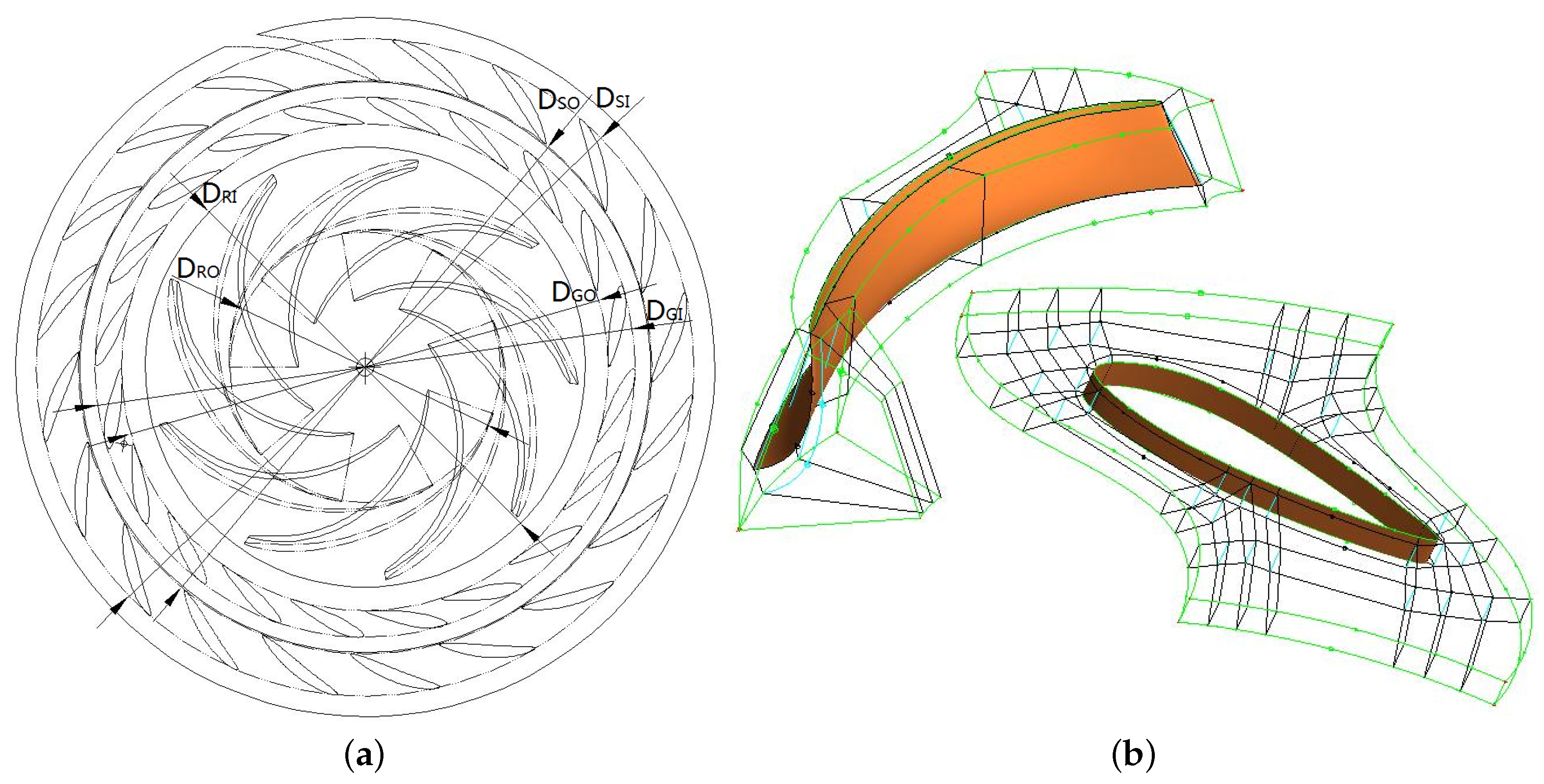
The computational domain consists of different zones: a runner composed of 9 backward blades, 20 guide vanes, 20 stay vanes, the volute and the draft tube. The main geometry features are reported in

Table 1. Main characteristics of the model for the considered analysis.

Runner Data				Guide Vanes Data					Stay Vanes Data
${\mathrm{D}}_{\mathrm{RI}}$	${\mathrm{D}}_{\mathrm{RO}}$	$B4$	${\mathrm{N}}_{\mathrm{RB}}$	${\mathrm{D}}_{\mathrm{GI}}$	${\mathrm{D}}_{\mathrm{GO}}$	$B3$	${\mathrm{N}}_{\mathrm{GV}}$	$a_3$	${\mathrm{D}}_{\mathrm{SI}}$	$B2$	${\mathrm{N}}_{\mathrm{SV}}$
300	185	48.85	9	475	389	48.85	20	24	725	48.85	20

; a representation of the geometry with the measurements of the main diameters is reported in Figure 2a; the characteristic parameters of the model include Q = 297 kg/s, H = 30 m, n = 670 rpm, at the design point. The geometrical model considered in the analysis is about a 1:11 scaled geometry of the test rig model dimensions.

The analysis aims to investigate the unsteady flow field in the pump turbine during the phase of rejecting load, through closing guide vanes. The flow close to the no-load operating condition becomes highly turbulent, dominated by backflow regions, with the formation of the vortex, and partial pumping flows start to form in the runner channels. Additionally, the fluid behavior is severely unsteady: the performances are affected by the continuous formation of recirculation zones, as observed in [24]. To set a realistic analysis, two requirements have to be fulfilled: the grid generation must be carefully carried out; meanwhile, the moving mesh technique requires a high quality definition of the guide vane domain.

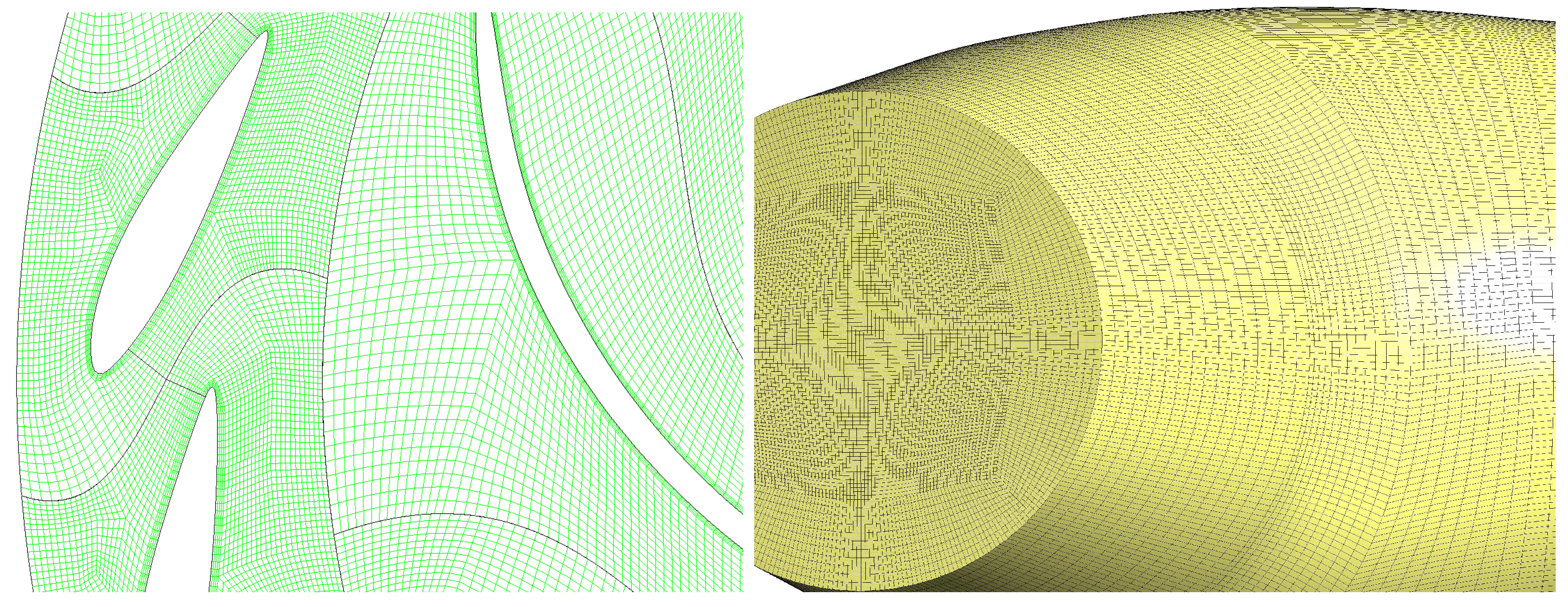
In order to increase the accuracy of the numerical solution, hexahedral grids have been adopted in the whole computational domain using structured blocks, except for the volute and the stay vane. The runner domain, composed of a hub, a shroud and seven backward blades, is defined by about 1.93 M cells, while the guide vane zone, made up of 22 vanes, contains 1.52 M cells; it is worth noticing that O-type grids have been adopted for both the blade zones (runner blades and guide vanes). Due to the requirements for an accurate analysis of the vortex, the hexahedral mesh is also adopted in the draft tube (1.42 M cells) and tetrahedral meshes are used for the volute and stay vane. Figure 2b illustrates the adopted topology for a runner blade and a guide vane, the connection between the different volumes is realized using interfaces.

Table 2. Mesh specifications of the model.

Characteristic	Runner	Guide Vane	Draft Tube	Volute and Stay Vane	Total
Type of Elements	Hexahedral	Hexahedral	Hexahedral	Tetrahedral	-
Number of Elements	1.93 M	1.52 M	1.42 M	1.79 M	6.66 M

illustrates the characteristics of the meshes adopted in the zones of the model.

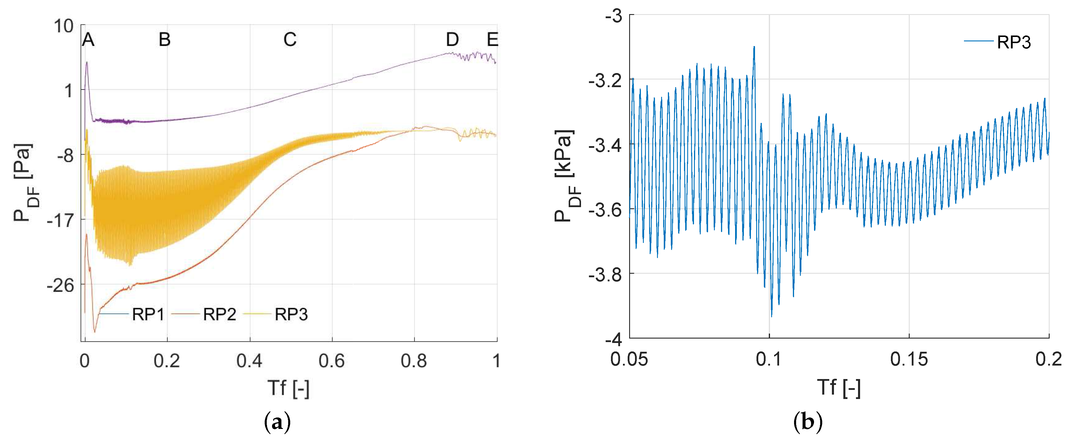
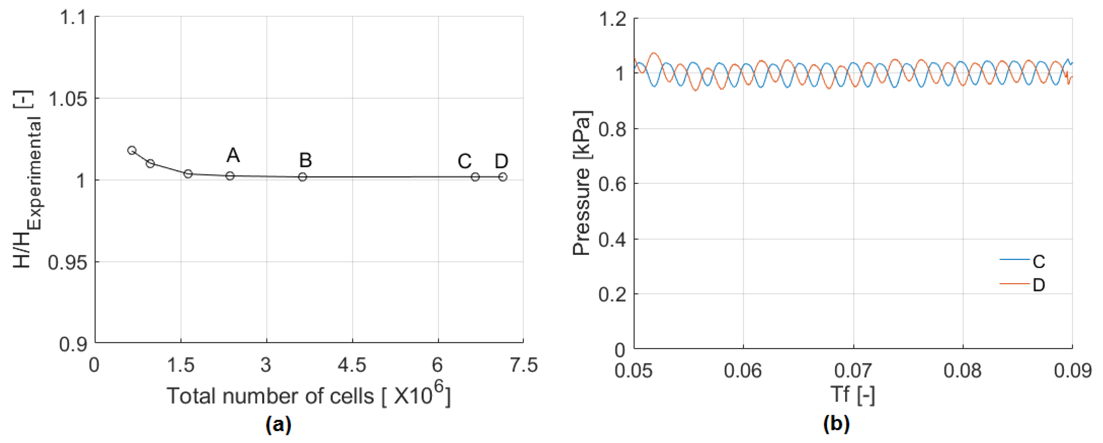
It is worth mentioning that, preliminary to the study, a mesh sensitivity analysis has been carried out by adopting five different grid sizes. The work is focused on the determination of the unsteady characteristics, and pressure pulsations are closely related to the unsteady flow.

The mesh sensitivity analysis, shown in Figure 3a, highlighted a mesh independent solution from about 2.36 M elements (Point A); however, the local pressure pulsations appear to be correctly evaluated only with total number of elements greater than 3.63 M (Point B). In order to guarantee the capacity of the numerical solution to capture local pressure pulsations well in the load variation process, the mesh was further subdivided (Point C: 6.66 M elements). For further mesh elements’ increase (Point D), the results demonstrate that approximately only a 0.25% divergence in the average value of pressure fluctuations was found; therefore, total elements equal to 6.6 M has been used in the proposed analyses. Figure 3b illustrates pressure fluctuations of monitoring Point R3 in the range of $Tf$ from 0.04 to 0.09. Finally, Figure 4 shows some details of the mesh in different regions of the model.

A method used for the computational analysis of a pump-turbine consist of re-defining the mesh for different configurations of the guide vanes; however, the procedure is affected by several problems and presents the drawback that only a few selected conditions can be simulated. For these reasons, in the adopted mesh-motion model, the grid is allowed to automatically deform based on 20 local coordinates: each guide vane can rotate around its own axis to change the position. Nonetheless, in the presence of large deformations, it might be difficult to modify the current mesh to avoid the generation of high-skewness elements. In order to ensure mesh quality during the moving of guide vanes, required for an accurate characterization of the flow field, the condition of a minimum face angle (α ≥ 30°) was imposed. The initial mesh presents a high quality with the minimum face angles of elements close to 90 degrees; furthermore, at the end of the closure period, at least 60% of the mesh elements still present the minimum face angles of about 90°, and the minimum face angle of other elements is larger than 30°. In order to both increase the volume and preserve the quality of the prismatic elements close to the border, the “specified displacement” has been adopted as the mesh motion method, and the mesh stiffness has been set, the setting allowed to absorb the main deformation far from the body. On the other hand, all guide vanes move to specified locations with the mesh motion laws: according to the ANSYS CFX options, upper and lower surfaces were set using the “unspecified mesh motion” method, whereas the inlet and outlet of the guide vane domain adopted the “stationary” condition. As reported in the ANSYS CFX-PRE Users Guide [25], the domain motion option “specified displacement” is defined as the domain displaces according to the specified Cartesian components, and using “unspecified mesh motion”, no constraints on mesh motion are applied to nodes. The movement is determined by the motion set on other regions: this allows one to move the nodes on the surface, if needed. Finally, when using “stationary”, the domain remains fixed in the absolute frame of reference. Meanwhile, another movement was also applied to the nodes belonging to vanes: they move along the vane profile in the opposite direction compared with the vane closure direction.

3. Numerical Model

In the last few years, as HPC resources have become available, a renewed effort in adopting the Reynolds stress models rather than reducing the turbulent eddies effects to a turbulent viscosity term has arisen. Reynolds stress models are computationally expensive, compared to a conventional one or two-equation models; however, they have been proven to archive a higher accuracy and better results under the correct flow conditions. Furthermore, according to Liu et al’s study [26], SSG Reynolds stress and k-ω models present larger deviation, and the relative error of the SSG Reynolds stress model is beyond 10%. The relative errors of k-ε, RNG k-ε, and k-ε EARSM models are lower, limited to around 2%. Specifically, the description of internal flow with k-ε EARSM has been demonstrated to be the most accurate. Finally, it is well known that reynolds-averaged navier–stokes equations (RANS) models cannot predict, with high accuracy, all flow details in each separated flow region [26]. The above reasons lead to the formulation of the solution strategy proposed in

Table 3. Solution strategy adopted for the analysis.

Analysis	Turbulence Model	Guide Vanes’ State	Iterations/Time Step
Steady	RNG $k-\epsilon$	Fixed	500
Steady	$k-\epsilon$ EARSM	Fixed	2000
Unsteady	DES	Moving	$4.975\ast {10}^{-4}$ s

. Two preliminary steady analyses have been run setting different turbulence models, the RNG k-ε and the k-ε EARSM. In the present work, the detached eddy simulation was used for the unsteady calculations where the steady-state results were adopted as initialization. In the simulation of the rejecting load phase, the guide vanes were moving using a specified closure law, and the time step $ts=4.975\times {10}^{-4}$ s, equivalent to a rotation of 2°, has been adopted.

The detached eddy simulation (DES) model was proposed by Spalart [27] in 1997 and first used in 1999. In recent years, DES has been successfully used in a large amount of cases including many industry applications [28,29]; it has proven to be more accurate in the presence of prominent separations in the flow domain and better able to capture the flow field details compared to other models [30,31,32]. Furthermore, the DES method has great advantages: it can be applied at high Reynolds numbers, and it is suitable to solve geometry-dependent, unsteady three-dimensional turbulent motions, similar to the large eddy simulation (LES) model. The model combines the advantages of the RANS (for the near-wall regions) and LES (used in the free-stream) models; consequently, it has the potential to offer more accuracy than RANS at less cost than LES [33].

The boundary conditions adopted for the model are reported in

Table 4. Boundary conditions used in the numerical analysis.

Patch	Boundary Conditions	Values
Inlet	Total pressure	294,300 Pa
Outlet	Opening	0 Pa (gauge)
Zone Interfaces	GGI	-
Wall roughness	Smooth wall	-

. The total pressure condition at the inlet is combined with the opening condition at the outlet, due to the presence of the highly disturbed flow field in the draft tube. The turbulence parameters are defined by specifying the turbulence intensity and hydraulic diameter. The solid walls are defined as no-slip: scalable wall functions are used in steady simulations, whereas under unsteady conditions, automatic near wall treatment is applied. Finally, three couples of interfaces among different domains are connected through the general grid interface method.

The analysis was run in a workstation in parallel mode using 32 cores (Intel(R) Xeon(R) CPU E5-2650 @ 2.00 GHz) and 128 Gb of RAM, and the computational time to analyze the whole unsteady process was about 20 days.

4. Closing Law of Guide Vanes during Load Rejection

The time needed during the shutdown operation of a pump turbine should be limited, due to the harmful effects of prolonged operation at shut-off. In fact, the energy of flow is converted into heat, and it results in a dangerous increment of temperature for both the fluid and the unit itself, at instant shut-off. For these reasons, it is necessary to use suitable laws to close the guide vanes in the unsteady operation. Wylie et al [34] introduced one-dimensional equations to govern the changes of guide vanes opening by describing unsteady pipe flow. Two dependent variables are considered, the centerline pressure $P=P(x,t)$ and velocity $V=V(x;t)$, where x represents the distance along the pipe and t is the time. The linear closing law has been later applied to various power plants characterized by adverse flow field effects; specifically, the laws of prolonging the closing time (fast-slow or slow-fast sequences [19,20]) were proposed according to different cases.

Dynamic stresses caused by hydraulic excitation lead the machine to operate in an unsafe state and affect the life of the unit with the long-term operations under special conditions. Especially in the load rejection phase, the magnitude of radial vibrations could greatly increase, resulting in the damage of the unit; as a consequence, it could not be restored to the initial conditions after loosing load. According to Liu et al. 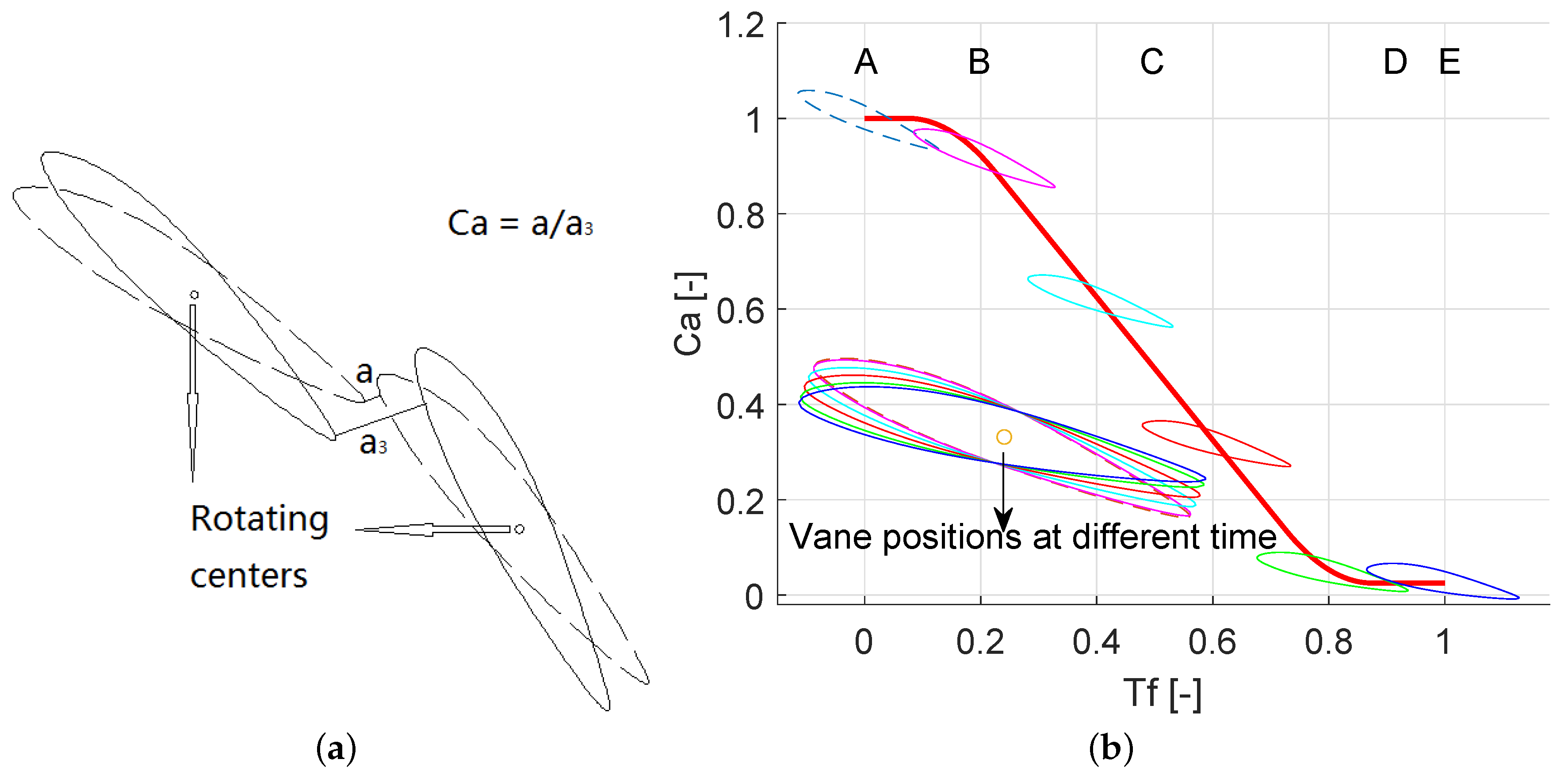[19], when the valid guide vanes’ closing time is longer, the volute maximum hydrodynamic pressure becomes smaller. Therefore, improved guide vanes’ closing methods for the normal operation of RPHES are very necessary, and a special closing rule, with five stages, is hereby proposed. The relative opening ($Ca$) of guide vanes is defined as the opening at best efficiency point (BEP) divided by the opening at the considered time, as illustrated in Figure 5a. Figure 5b shows the variation of the relative opening with the closing law.

The proposed closing method was built by combining steady-state test data (obtained from Xiangshuijian pumped storage plant [15]) and unsteady simulations under fixed conditions. In order to reproduce the real flow state and analyze the influence of the unsteady flow, each guide vane was continuously and independently adjustable. It is worth mentioning that $Ca$ was not equal to zero at the total closure point, for reasons related to the manufacturing precision: guide vanes experience abrasion after the units run for a long time, and a relatively small gap remains at closure. Therefore, the ideal state of $Ca=0$ and the $Q=0$ kg/s are not realistic; on the other hand, in ideal conditions, the flow is zero when guide vanes are completely closed. In this case, the fluid is divided into two separate parts by guide vanes; furthermore, it is impossible to guarantee the high quality of the structured mesh when guide vanes are completely closed, especially for dynamic mesh motion. Consequently, the process of load rejection lasts about 6.41 s (valid time) after five stages, and the relative opening of guide vanes results in 6.85%. The numerical data were acquired after six revolutions, when a stable convergence was reached, and during this period, 79 complete impeller revolutions were completed to achieve the whole operating process. All simulations were carried out on the HPC with efficient parallelization, and two nodes of an HPC cluster were used in the unsteady simulations. The computation time per each revolution is about six hours with the mesh C (Figure 3a).

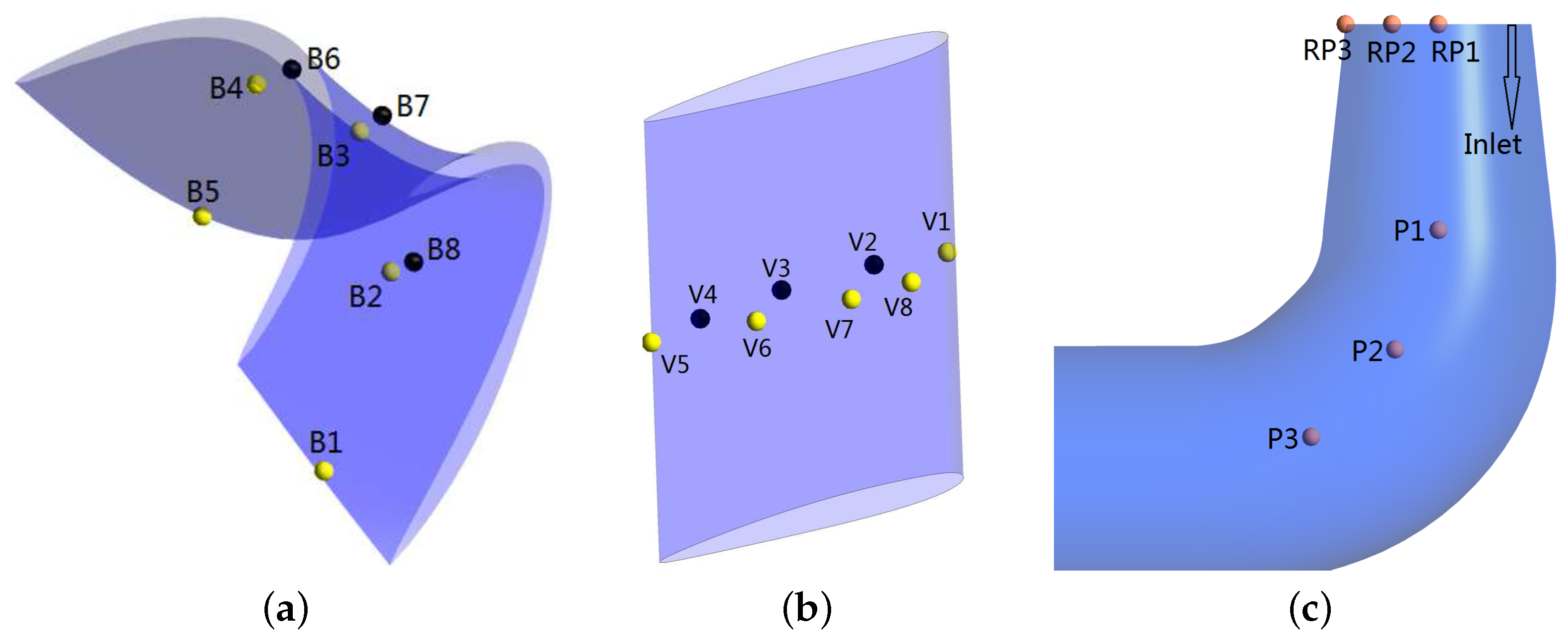
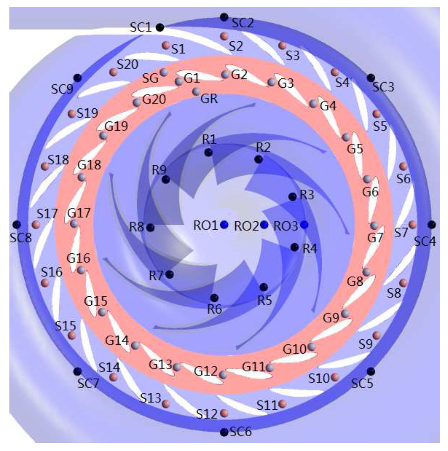
Different monitoring points have been chosen in order to probe the variations of the hydrodynamic variables during the analysis, as will be better clarified in Section 6. Figure 6 and Figure 7 provide a schematic representation of the locations of the monitoring points used in the blade, guide vane and draft tube domain.

5. Validation of the Numerical Model

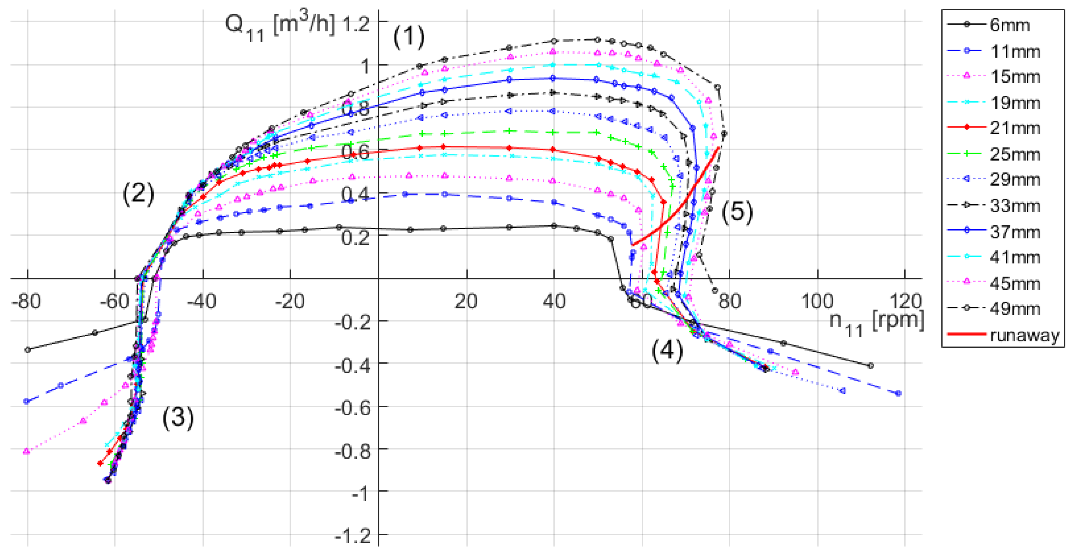
The numerical model adopted for the analysis represents about a 1:11 scaled geometry of the considered machine: the pump turbine was initially designed for the pump condition and tested for the turbine condition. The experimental campaign was carried out at Xiangshuijian pumped storage plant [15]. Figure 8 shows the characteristic curves of the machine for different values of vane openings: the rotating speed was measured using a counter to register the number of complete revolutions of the shaft (n) with an accuracy of $\pm 1$ rpm; the values of the pressure were measured by transmitters and discharges were obtained from electromagnetic flowmeters. The calibration of the instruments was performed on site. The instruments’ precision can be described by the total accuracy of the experimental stand: the error of the hydraulic comprehensive experiment bench is less than 0.25%, as reported in [35].

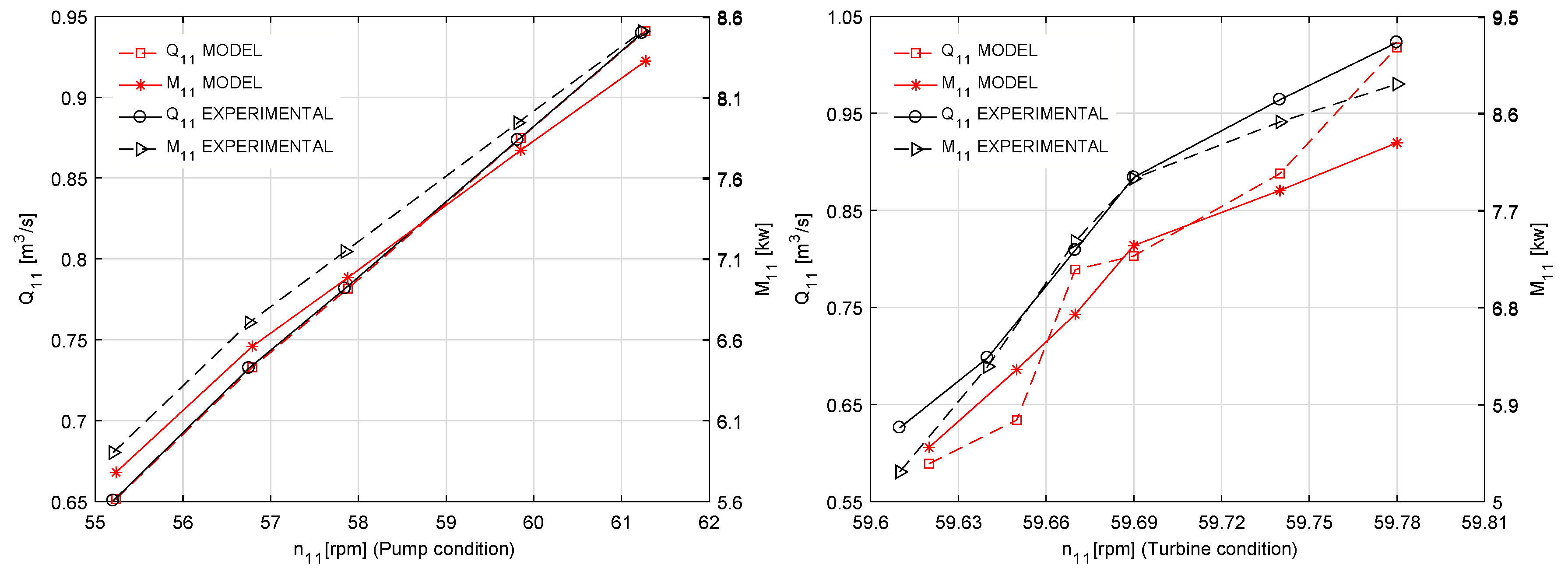
Computational analyses were carried out at different guide vane openings and compared with experimental data in order to assess the accuracy of the proposed model. As Figure 9 shows, the calculated curves are in agreement with the experimental data.

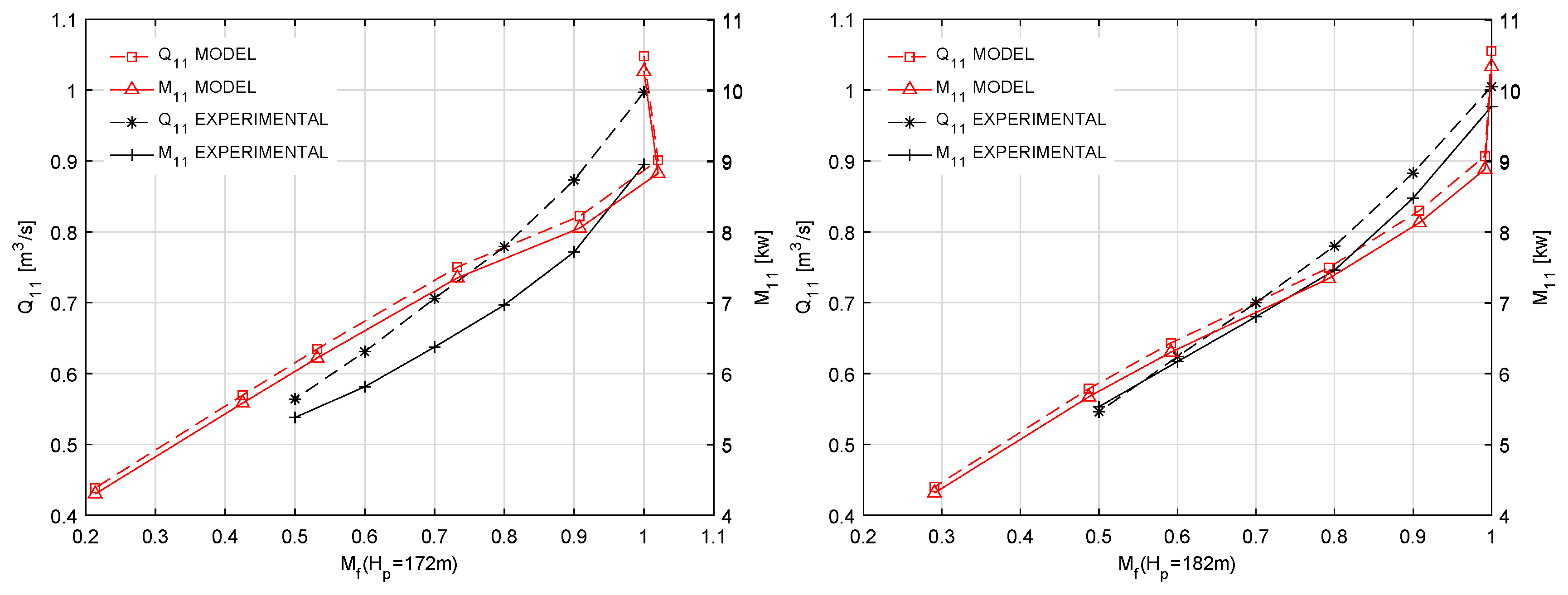
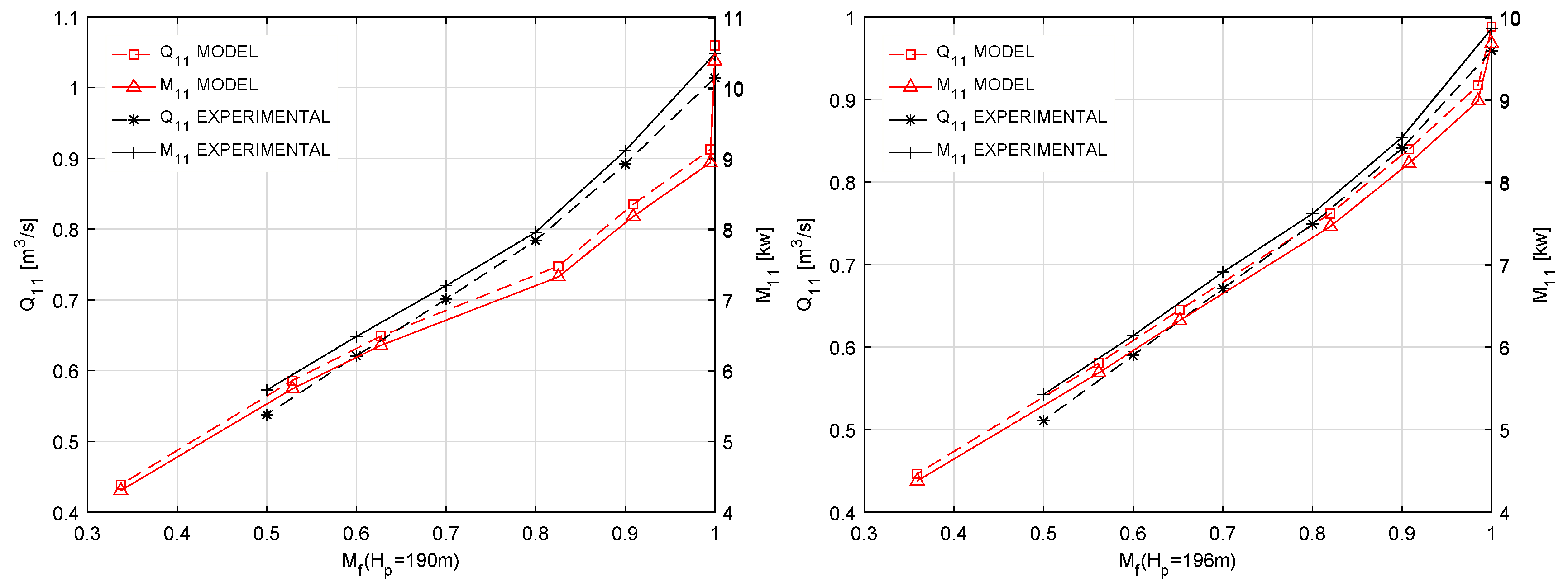
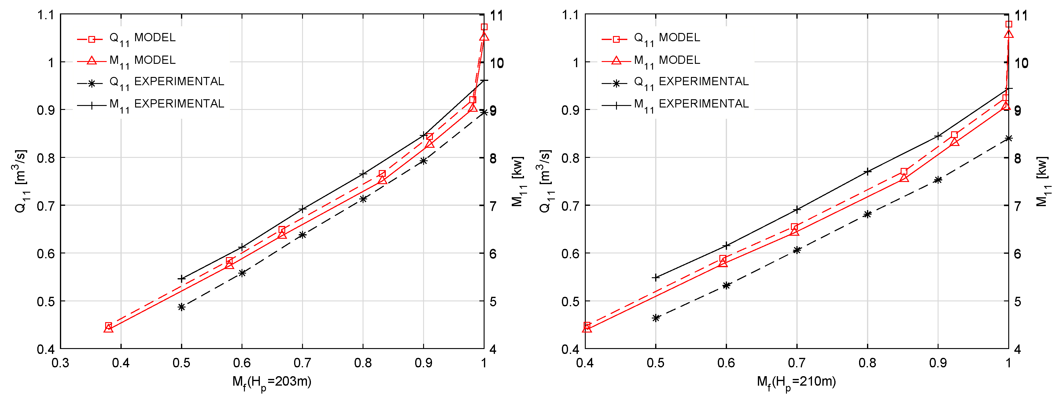
From Figure 10, Figure 11 and Figure 12, the validation for turbine mode is further investigated: the results are in accordance with the measured data; the values of $Q_{11}$ are close to the experimental data, whereas $M_{11}$ presents errors of about 2% for the considered vane openings (near the design point). On the other hand, points far from the design condition present larger differences of $M_{11}$ and $Q_{11}$; however, the errors in terms of $M_{11}$ are lower than 11%. Considering the discharge capacity, the maximum error is about 13%, when the machine works in extreme off-design conditions. It can be concluded that the numerical model is accurate to properly describe, for most of the working conditions, the physics of the considered unit.

6. Results and Discussion

The results of the numerical simulation are presented, in the following sections, in terms of flow field analyses of the different zones. The uncertainness of the model must be taken into account to correctly evaluate the results; as reported in Section 5, the uncertainty of relevant indicators as $M_{11}$ and $Q_{11}$ in both pump and turbine modes was less than 2% for the conditions near the design point and up to 13% for extreme off-design conditions, near the guide vane final closure point.

6.1. Flow Field Evolution in Draft Tube

In order to describe the evolution of flow field in the draft tube, the pressure signals acquired from the monitoring points have been collected during the load rejection cycles.

Figure 13a reports the pressure fluctuations measured in three different positions along the radial direction on the draft tube inlet (Points RP1, RP2 and RP3), during the shutdown phase (the time factor $Tf$ represents the time t normalized with respect to the total time T of the load rejection process). The maximum pressure pulsation of the pipe inlet in the steady simulation at BEP resulted in being about 15% of the set value. However, as for unsteady simulations, the inlet pressure in the draft tube suddenly increased by about 10 kPa at the beginning of closure phase. The turbulence decreased with time, and the flow field became more regular; this contributed to the stabilization of pressure at about $Tf=0.035$ with an increasing trend until $Tf=0.97$. Finally, the pressure value reached a peak, and small fluctuations were registered in the last stage.

As shown in Figure 13, the most significant pressure fluctuation was registered at Point RP2, and it becomes more stable over time: this was caused by the formation of two small vortices around the center of draft tube inlet. The pressure amplitudes at the operating condition with 100% load resulted in being about 10-times larger than the last closure phase (Figure 13a), the main reason being the formation of three-dimensional unsteady flow structures in the draft tube. In addition, the flow evolution during the period of load rejection can be characterized in order to determine the hydrodynamic conditions causing pressure oscillations with consequent vibration in the component of the machine [36].

Figure 13b illustrates in detail the pressure pulsations at RP3 during the transition between the operating points, from $Tf$ = 0.05–0.20: small pressure variations can be clearly observed during the load rejection cycle, and the maximum fluctuation range is about 0.7 kPa. Figure 14 reports the spectral analyses of signals acquired from monitoring points in the straight cone and elbow sections: the analysis of the pressure fluctuations at RP2 detected the runner rotating frequency ($S_t$ = 0.6763) corresponding to the formation of vortices (the peak in Figure 14); however, the spectrum in Figure 14b proves that the resulting harmonic frequencies of pressure fluctuations in the elbow are not influenced by the runner rotation directly in the draft tube.

Finally, in Figure 15a, the evolution of the pressure field in draft tube is presented for three different instants in time: the tangential velocity in the draft tube caused the formation of two vortices, and the resulting pressure fluctuations in the straight cone and elbow sections. Furthermore, the nine lower pressure regions at the wall of the draft tube cone were caused by the rotation of runner, and they were related to the passage of the blades and the development of their wake.

6.2. Analysis of the Runner Flow Field

Figure 16 reports the evolution of the pressure signals measured at the representative points of the runner domain (Figure 6 and Figure 7); as can be observed, the pressure changes assumed a similar trend for the points of the same circumferentially symmetrical positions. At 100% load (BEP condition), the turbine operation was stable, and no high amplitude frequency could be observed. With the changes from quadratic to linear of the closure law function, an increase of the pressure value was registered in the runner domain, as shown in Figure 16.

Pressure values on the surface of the blade (points from B1–B8) during the load variation cycle are provided in Figure 17a. As expected, the pressure pulsations were strongly perceived at the blade leading edge (Point B1), due to the proximity of the guide vane outlet; the values firstly increased because of the changes of the incidence angle; later, they slowly decreased until $Tf=0.95$. Finally, pressure at B1 assumed the same value of B2: considering the position of B2, as the original hydrostatic head speed change was relatively large, the hydrodynamic head was converted into the hydrostatic head, which contributed to the increase of the pressure value. On the other hand, the areas in the proximity of the considered blade-span, on both sides, represented the main work areas; in the zones, the pressure energy was more quickly transformed into dynamic energy than the other parts of the blade. B8 represents the corresponding point on the blade suction surface at the span-wise coordinate of B2: the pressure drop at this point was significant, and an high positive work was registered.

At about half-span of the blade profile (monitoring Points B3 and B7), the pressure values decreased by about 25%. In the next considered section, the trend of pressure was in contrast: pressure at B4 decreased, whereas pressure at B6 had been increasing: this fact explains the formation of an unstable flow field near the suction surface, close to the runner outlet. The closer to the blade trailing edge, the greater the pressure difference between the blade pressure surface and the suction surface at the corresponding positions (Figure 17a): it can be observed that the pressures values at Points B4 and B6 were greatly reduced after loosing 28.7% load ($Tf=0.43$). The increment of pressure at B5 was smaller than B6; however, the amplitudes of the pulsation were the largest compared to other points from the beginning to $Tf=0.40$. The main reason is the development of a swirling wake in the draft tube, even though the dominating flow phenomena in the runner was composed by pressure fluctuations related to the flow field in the guide vane domain. Moreover, the blade passage frequency ($S_t$ = 0.6763) was also captured (Figure 16b).

Figure 17b illustrates the trend in the torque on the runner blades. As mentioned before, after the guide vanes’ closure, a small quantity of water flowed into the runner from the guide vanes (not the null discharge condition). As the closure phase was completed (relative opening of 6.85%), the torque amplitudes of blades oscillated in a range of ±0.15 Nm. The amplitudes were also in a small range compared to the fluctuations in the pressure measured in the different zones of the model; hence, the closure law can be considered suitable for the model. Moreover, based on the data of Cavazzini et al. [37], the limited range of pulsations involved positive consequences on the fatigue resistance of the mechanical components compared with the closing laws adopted in existing technologies.

Finally, in order to better illustrate the pulsations of the torque of the blades during the transition phase, Figure 18a shows in detail a time range of 0.2 s. Similarly, Figure 18b represents the torque variations of guide vanes in the period of T = 0.20–0.25 s: the torque amplitudes were limited to a very small range, which is beneficial to contrast the occurrence fatigue phenomena.

6.3. Analysis of the Flow Field in the Guide Vane

As observed, the changes of the flow pattern in the guide vane domain and the related enlargement of unstable area with the increasing dimension of vortices caused different phenomena:

• Torque pulsations in guide vanes
• Pressure oscillations
• Mass flow fluctuations

Figure 19a displays the variation in the torque values on guide vanes: the overall trend indicated a slightly increasing tendency until 70.44% load and a consequent reduction. In Figure 19b, the flow rate variation is presented for some guide vane channels: the decreasing magnitudes of discharges are similar, and the mass flow in each channel assumes the same progressive and regular reduction, as found in the numerical model. Due to the limited amount of mass flow at the end of closing phase, the amplitudes of the observed fluctuations increased with the intensity of the unsteady phenomena.

6.4. Water Ring Zones during Load Rejection

The trends of pressure PSD acquired from points in the circumferential direction of guide vane domain (Figure 20) had similar characteristics compared to the monitoring points of the runner. Figure 21a shows pressure coefficient values of points on the guide vane (as indicated in Figure 6): the registered values (at Points V2, V3 and V4), after an initial oscillation, kept a downtrend until the end of the closure phase. Specifically, the pressure values acquired at the leading edge (Point V1) and the trailing edge (Point V5) assumed a growing trend from about $Tf=0.8$, due to influence of the vaneless regions. In the leading edge zone, the pressure at V1 started to increase (after loosing 81.02% load) because of the proximity between guide vanes. At last, the pressure was equivalent to the initial value; in addition, it was affected by the flow field in vaneless space between the stay vane and the guide vane. The flow streamlines in the water ring zones are illustrated in Figure 21b.

Figure 22a presents the fluctuations in pressure values at the monitoring points SG and GR (in vaneless spaces, as indicated in Figure 7). For both points, the pressure values remained constant from the BEP for a short period (until about $Tf=0.1$), and a counter-trend in pressure values was found in the whole process: the pressure at point SG increased, while at point RG, a downward trend was registered. Compared with the operating condition at 100% load, the final pressure value at SG was increased by 9%, whereas the pressure at RG dropped to approximately 73%. In order to highlight the pressure pulsations at Point SG, Figure 22b illustrates the 0.20–0.21 range of $Tf$, where the change of amplitudes can be observed more clearly.

The vaneless space between guide vane and runner increased during the shutdown phase; as a consequence, the rotor-stator interaction was reduced. Most of the high pressure flow energy was dissipated rather than converted into mechanical energy; hence, the hydrodynamic moment decreased in runner (Figure 17b). Furthermore, the water ring was thicker due to the high values of the pressure gradient in the guide vane regions, and centrifugal forces, generated also with the contribution of the rotation of the runner, appeared in the guide vain domain. In addition, the inflow angle at the blade leading edge became greater, while the spacing between blades was reduced; the phenomena led to larger centrifugal force, which caused the growth of the water ring thickness. The formation of the water ring, consequent to the gradual closure of guide vanes, was the main reason that prevented the water from flowing into the runner domain and represented an obstacle to an efficient power production.

6.5. Analysis of 3D Streamlines in Passage

At the beginning of unsteady simulation, the calculated head resulted in being 29.35 m, whereas in steady simulation, it equaled 30 m at BEP: the difference was due to the sudden change of pressure at the inlet and outlet when guide vanes were closed, and it might be influenced by numerical unsteadiness. Figure 23a illustrates the changes of the head value in both the guide vane and runner. It is necessary to mention the oscillations of the two values of the head, caused by the changes in the flow rate and the influence of the mass moment of inertia. During the short period of time, the runner head was proportional to the square of a flow rate: the flow was slightly affected by the changes of the inflow angle; hence, the turbine power increased. The head of the guide vane increased more than twice compared to the initial value. Water flowed through a long duct to the volute and reached the guide vane area, where the head increment was related to the simultaneous decrease in mass flow (Figure 19b). However, as the part produced effective power, the runner head reduction was mainly caused by the pressure difference between the inlet and the outlet of the runner.

In the first stage of closure, the flow was regular, and no vortex could be found in passage, except for a small amount of swirls in the straight cone section of the draft tube, significantly influenced by the rotation of the runner and by the flow pattern at the runner outlet. However, the phenomenon was gradually perturbed by unsteady vortices in runner channels, and it finally blocked the passage (as shown in Figure 23b).

In Figure 24, the evolution of the internal flow field in the runner domain at two particular moments is analyzed in terms of streamlines’ evolution. From $Tf=0.21$, the presence of small recirculation zones was observed close to the pressure sides of the blades, and unstable flow in runner passages gradually developed, with flow separations. The flow in the former two-thirds of the runner channels was perturbed by the appearance of detachments, depending on the guide vane flow field evolution during load rejection. However, from $Tf=0.55$, the influence from the water ring caused a chaotic flow pattern and the growth of strong vortices near the runner inlet: in the zone, the flow became more unstable, and the back wave appeared in most of the flow paths. As for the regions close to the blades’ trailing edges, the flow pattern was relatively stable compared with the front parts. On the other hand, the mass flow reduction caused the development and enlargement of the regions affected by flow separations; further reductions of flow led to a full blockage of runner passages.

Initially, the formations of the stationary and rotational vortexes had the same physical causes, depending on the mean convective acceleration in the channels; whether the vortex formations would rotate or not, both phenomena led to an unstable characteristic. In addition, a small zone characterized by turbulent flow could be noticed close to the suction sides of runner blades. Subsequently, large attached eddies extended to the high pressure sides, and secondary vortexes appeared at the trailing edge, accelerating the process that led to the flow channel obstruction (Figure 24c).

The continuous increment in flow velocity was registered close to the runner outlet; the high velocity flow directly worked on the blades and generated larger dynamic moment. As noticed in the analysis of pressure fluctuations at the runner outlet (Figure 13a), the turbulent flow directly spilled into the draft tube, and vortices originated in the straight section of the draft tube.

The flow fields in the volute and stay vane were more stable, compared to the other domains, as shown by the trend of pressure at the monitoring points in the volute and stay vane (Figure 25).

In the proximity of the final closing point, the reverse flow appeared in the whole passage with an increment of magnitude (Figure 19b). In the vaneless space between the fixed and guide vane, significant swirls appeared, while the flow pattern in the volute did not follow the walls, resulting in shock loss (Figure 26).

Figure 26 shows the streamlines’ paths in the domains, including the volute, stay vane and guide vane at $Tf=0.97$; it should be noticed that the water only flowed through the part of the stay vane corresponding to the volute nose position; in fact, the other passages to the stay vane were blocked by the presence of vortices. Meanwhile, the flow from the stay vane was rejected by the guide vane due to the closed configuration; hence water flowed along the circumferential direction and entered in the vaneless gap between the stay vane and the guide vane. Moreover, the instabilities could have caused the vibrations of the unit.

7. Conclusions and Future Works

The unsteady phenomena in the reversible pump-turbine have been analyzed through the use of automatic mesh motion where the guide vanes’ movements are realized through the adoption of dynamic mesh based on a given closure law. The results demonstrate the good accuracy of the model in the description of the internal flow field, and the unsteady flow evolution in each domain can be continuously observed for different openings.

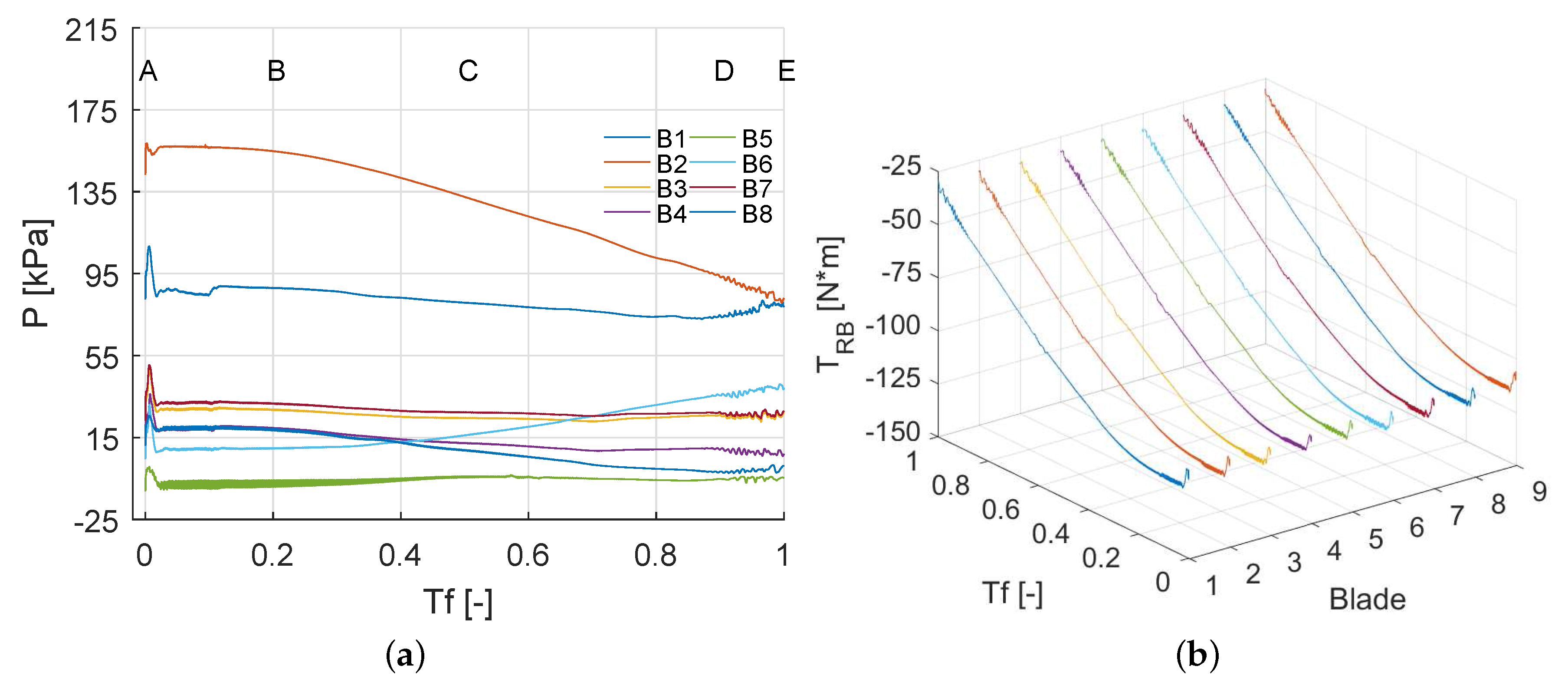
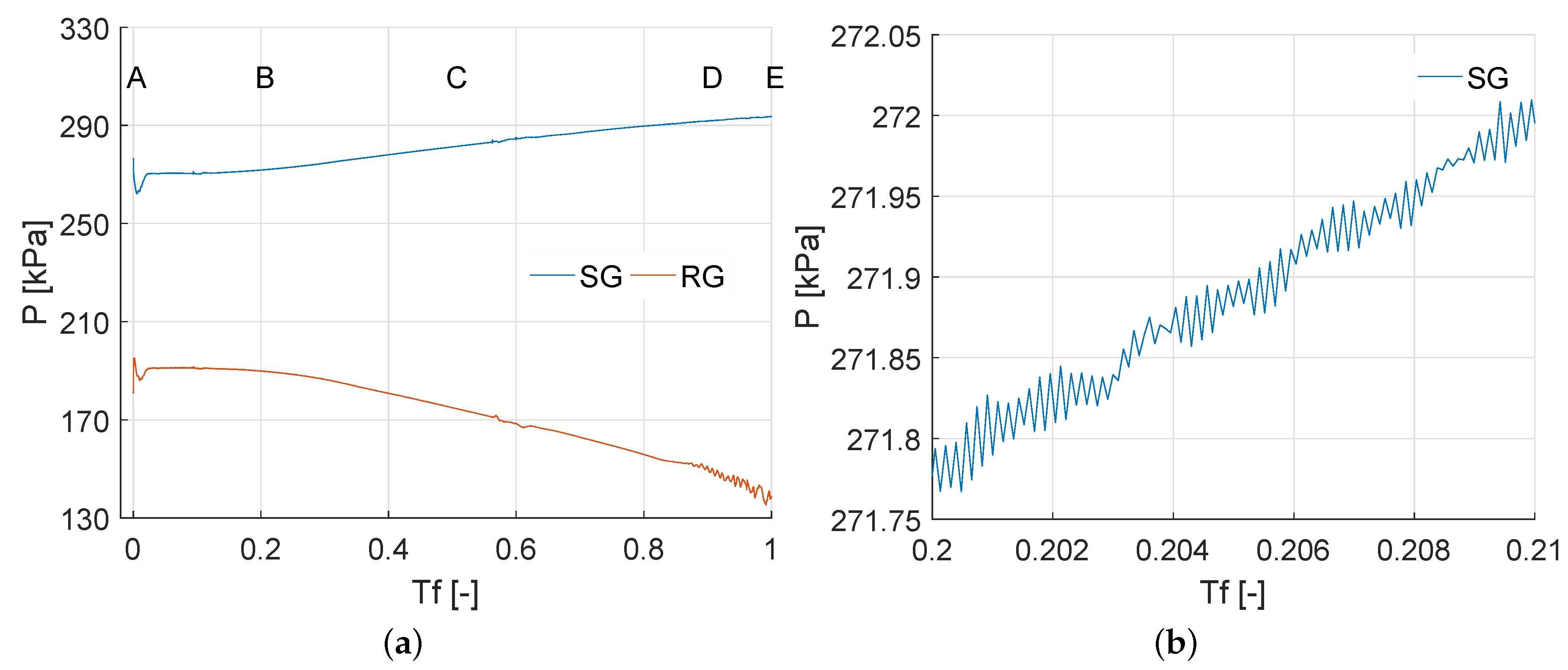
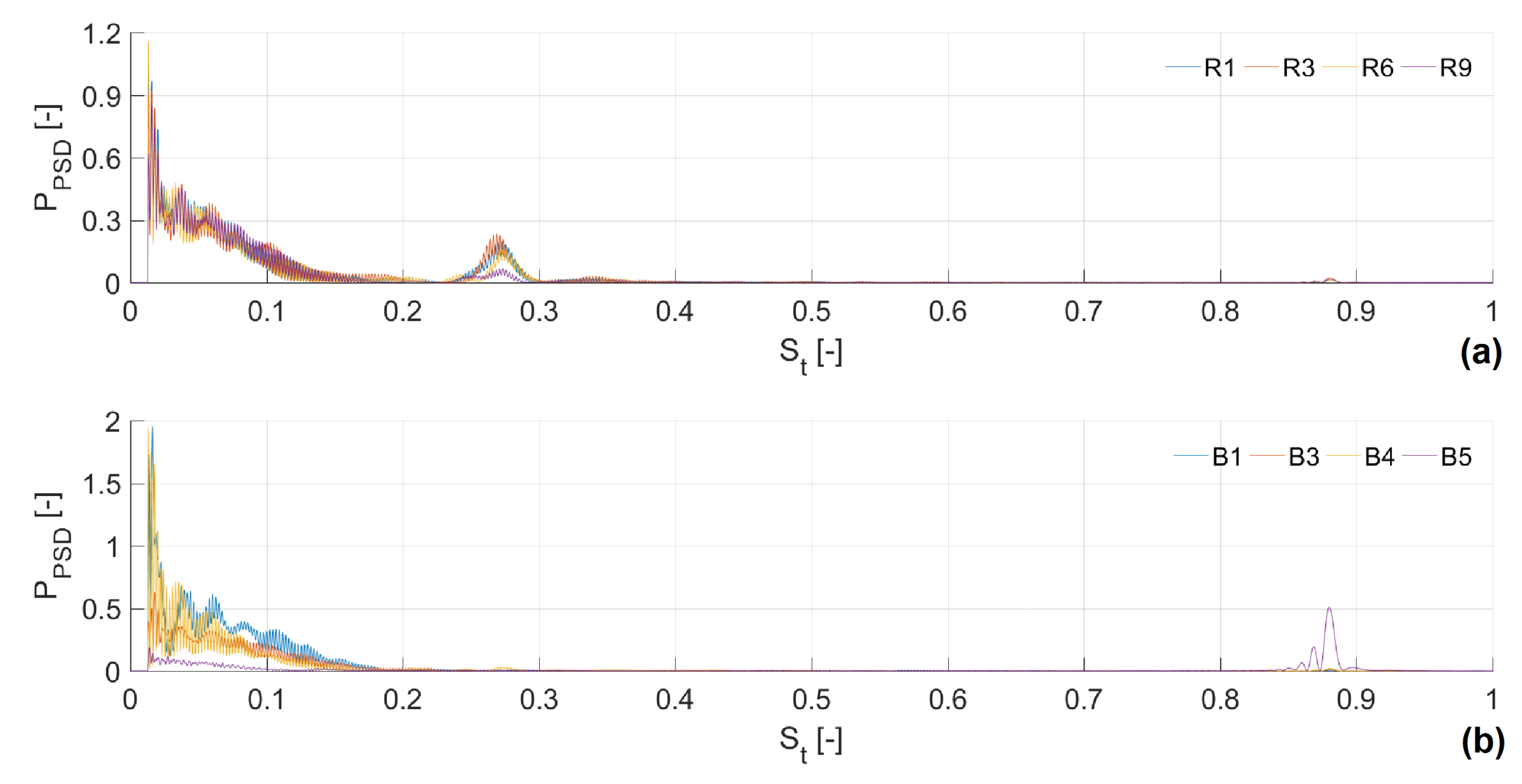
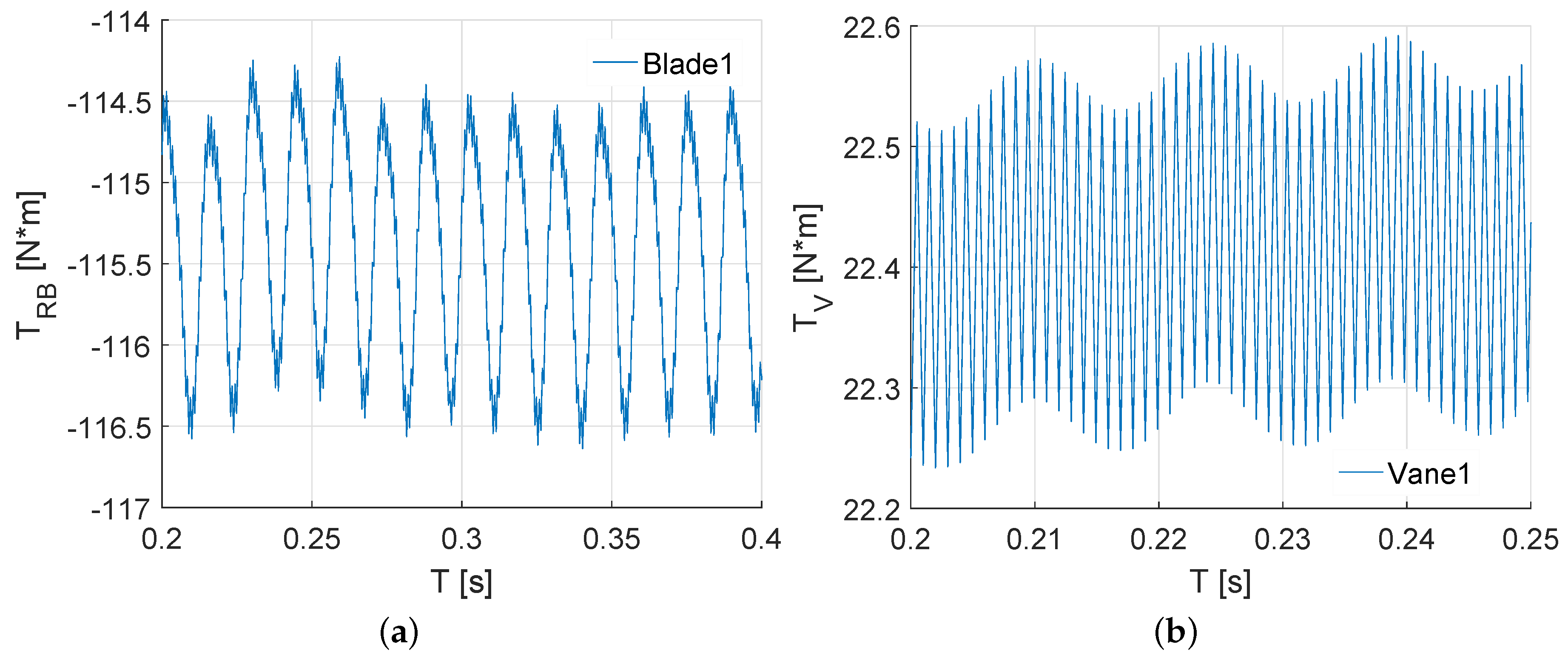
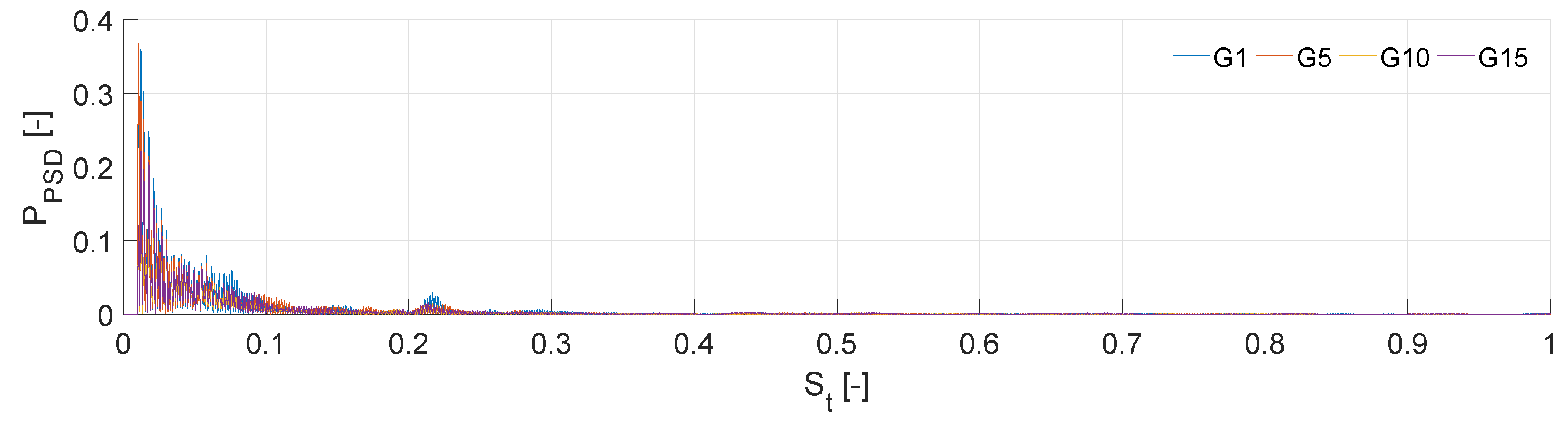
Signals from monitoring points have been analyzed focusing on the unsteady flow characteristics; the values of the mass flow, torque and pressure fluctuations are considered in both frequency and time-frequency analyses. The development of vortices has also been identified during the continuously dynamic guide vanes’ motion. The comparison of the results with experimental data proves that the closure law is suitable to model the unsteady phenomena.

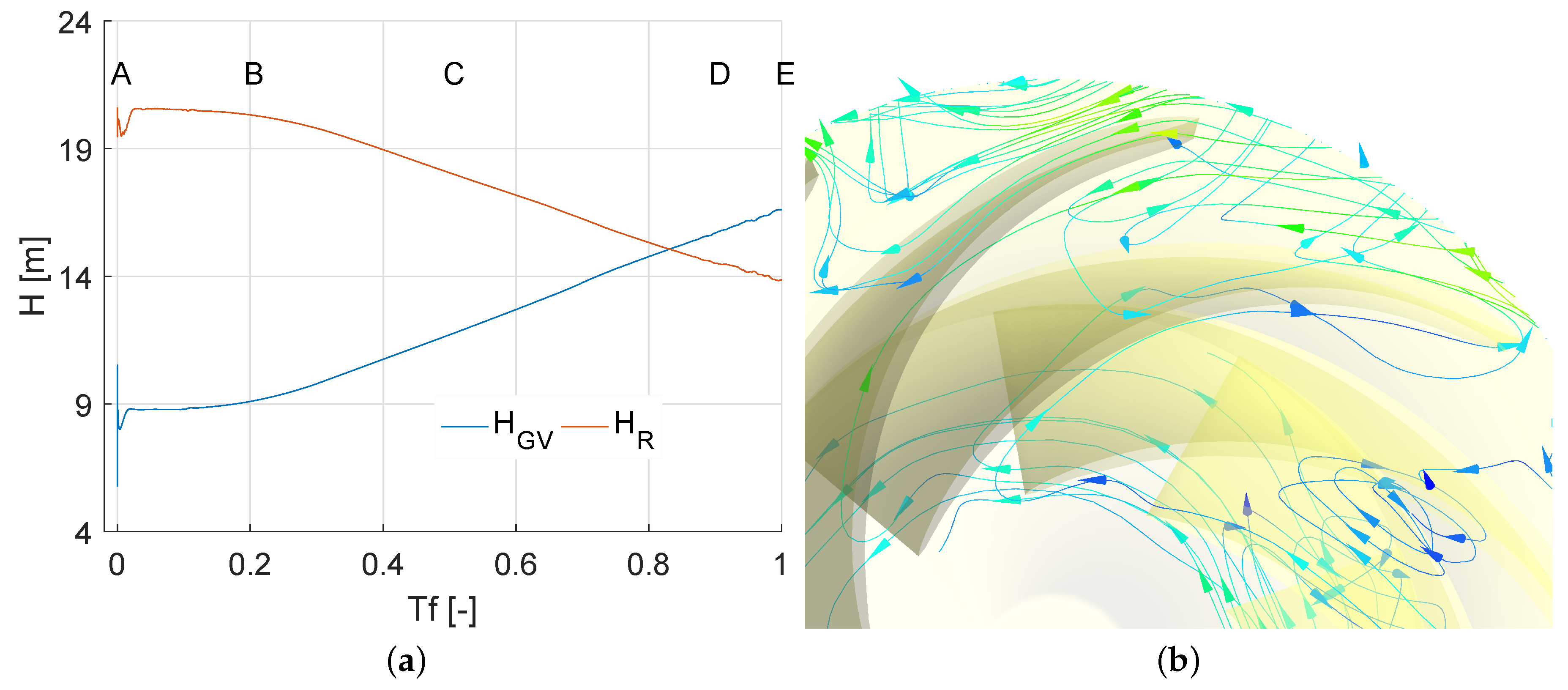
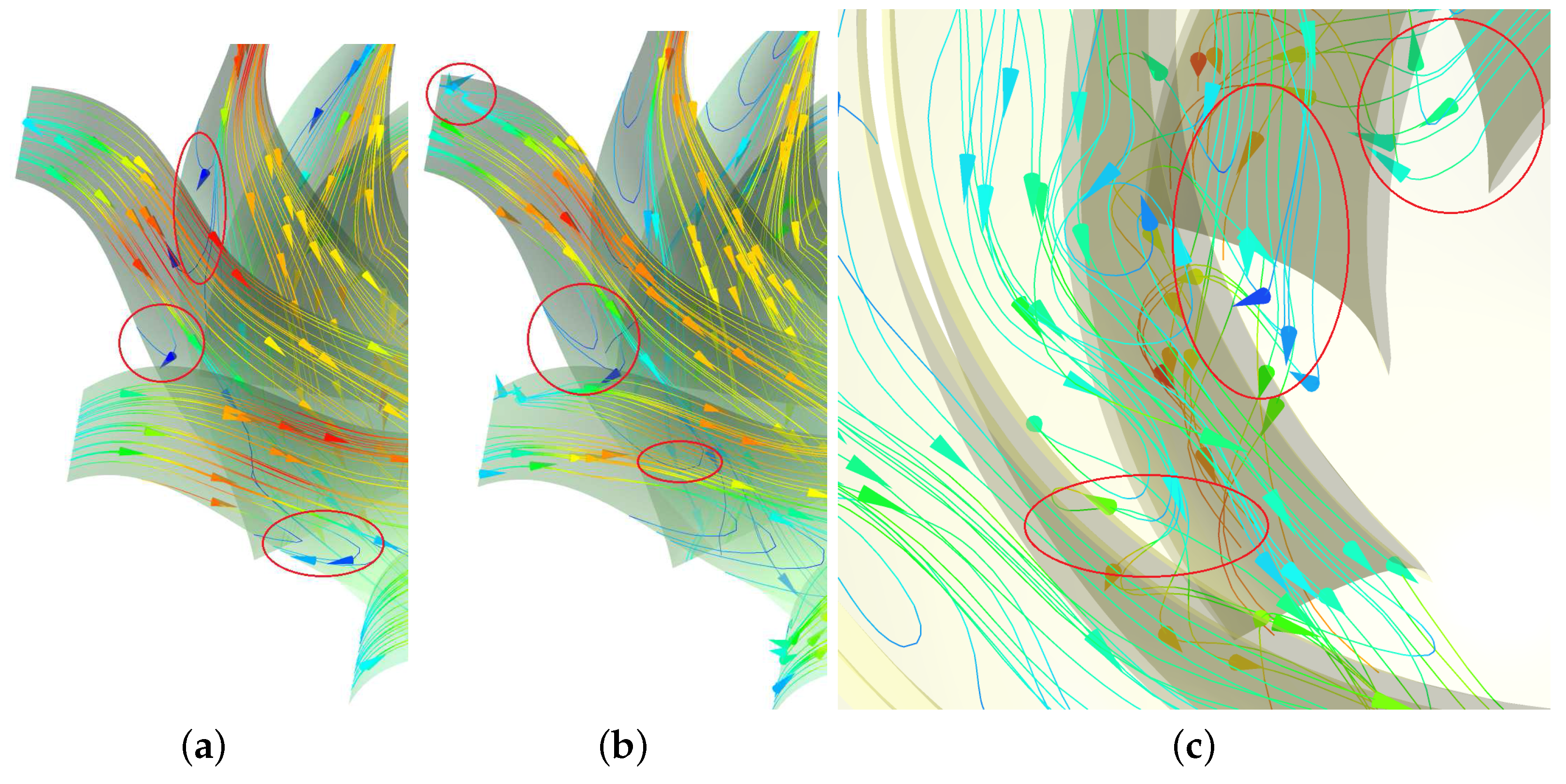
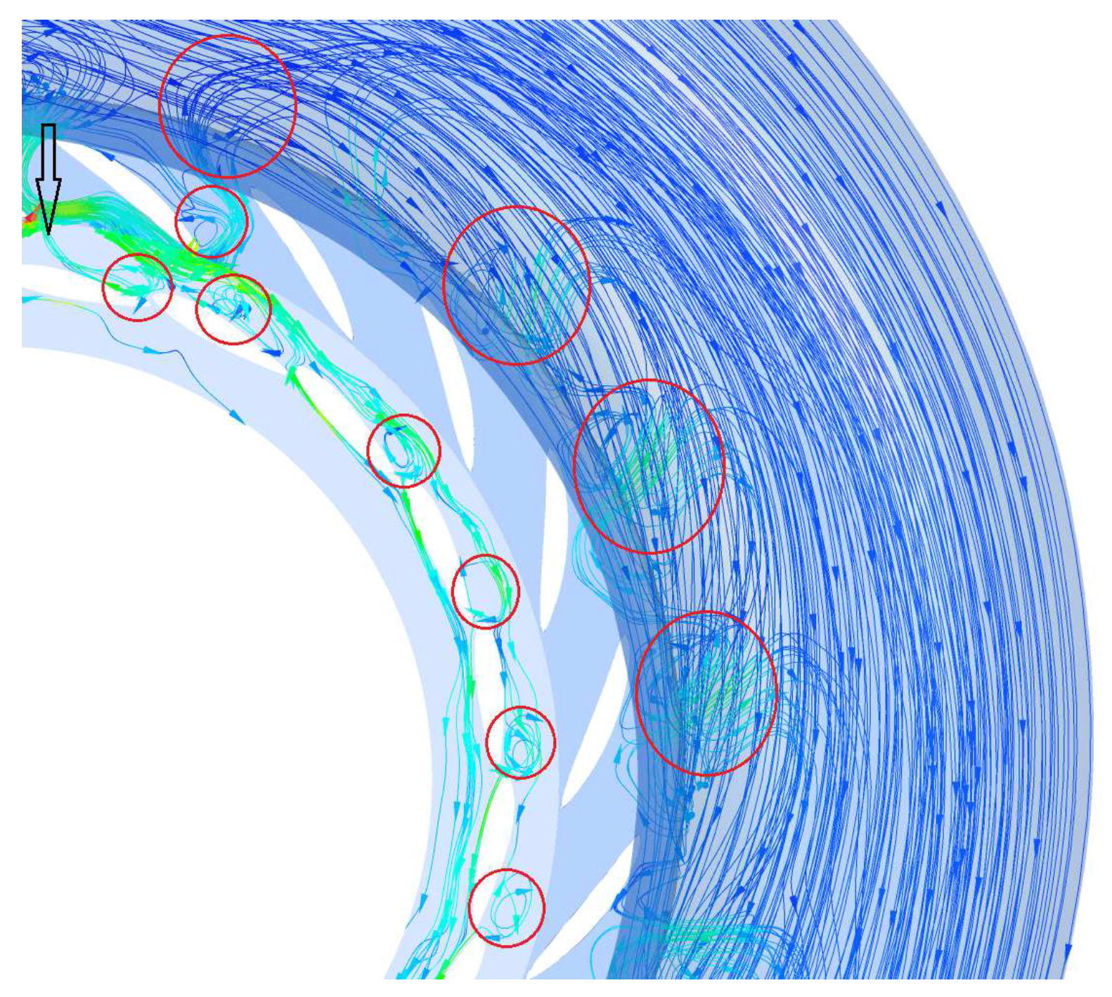
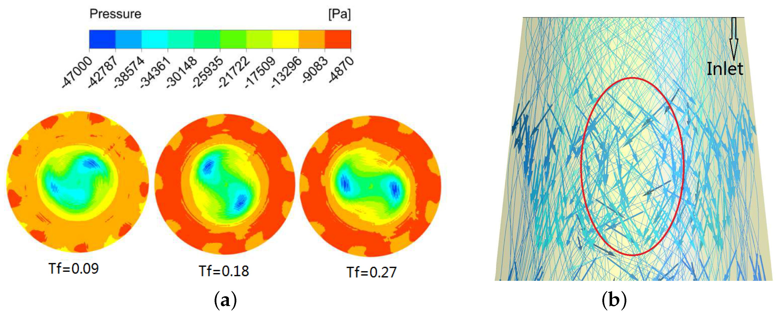
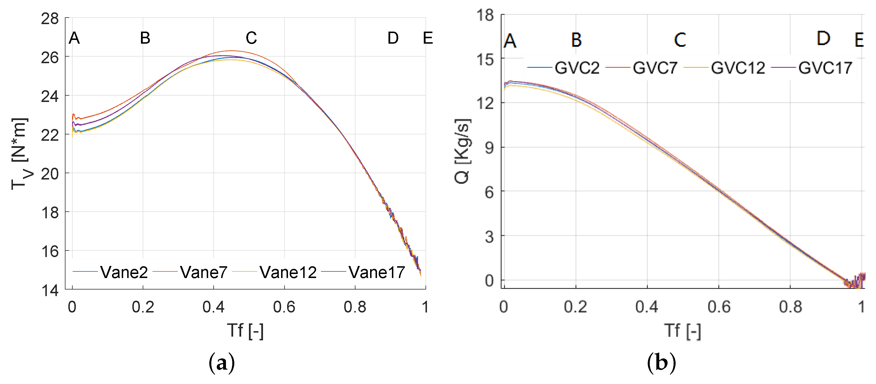
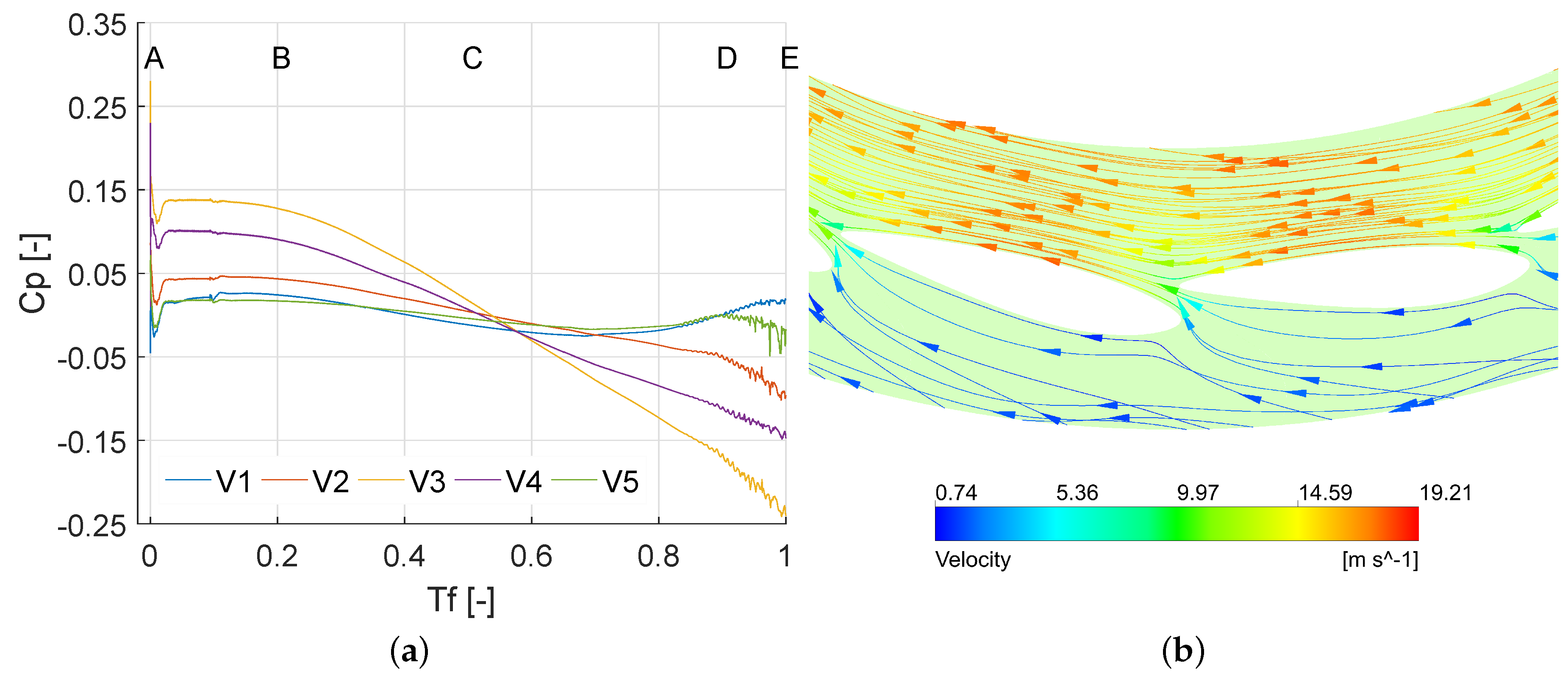
The mass flow value in the guide vane channels decreased with the smaller throat diameter, and this led to the fluctuations of pressure, head and torque. Furthermore, the water ring in the vaneless spaces gradually grew and became thickened; furthermore, it circumferentially rotated in the direction of the runner. Results showed how the formation of the water ring represented one of the main reasons for the vortex transitions between the runner channels. In addition, the flow evolution in the draft tube during the period of load rejection could be characterized in order to observe and identify the different scale of vortexes leading to different magnitudes of vibrations in the machine. In the proximity of the closing point, a significant reverse flow was registered in the guide vanes; in the space between the fixed and guide vanes, significant swirls appeared, and as a consequence, the water in the volute did not flow along the walls, resulting in shock loss. The present analysis is overall in a good agreement with the other models proposed in the literature, and it can be also applied to different reversible pump turbines under generating mode. However, the analyses of the development of unsteady phenomena were not sufficient for the determination of the S characteristics.

Future studies could also include the analysis of vibrations during the whole dynamic movement of guide vanes, an aspect strictly related to safely issues and, hence, to the life of the unit. Furthermore, the analysis of the noise is also an important aspect to be considered; these implementations will be part of the next research stage, following a similar approach, which has been proven in the previous work [36].

References

1. Barbour, E.; Wilson, I.A.G.; Radcliffe, J.; Ding, Y.; Li, Y. A review of pumped hydro energy storage development in significant international electricity markets. Renew. Sustain. Energy Rev. 2016, 61, 421–432. [Google Scholar] [CrossRef]
2. Beevers, D.; Branchini, L.; Orlandini, V.; Pascale, A.D.; Perez-Blanco, H. Pumped hydro storage plants with improved operational flexibility using constant speed Francis runners. Appl. Energy 2015, 137, 629–637. [Google Scholar] [CrossRef]
3. Fisher, R.K.; Koutnik, J.; Meier, L.; Loose, V.; Engels, K.; Beyer, T. A Comparison of Advanced Pumped Storage Equipment Drivers in the US and Europe. In Proceedings of the Hydrovision International 2012, Louisville, KY, USA, 17–20 July 2012. [Google Scholar]
4. Staubli, T.; Senn, F.; Sallaberger, M. Instability of pump-turbines during start-up in turbine mode. In Proceedings of the Hydro2008: International Conference and Exhibition, Ljubljana, Slovenia, 6–8 October 2008; Volume 9. [Google Scholar]
5. Zhang, H.; Chen, D.; Wu, C.; Wang, X.; Lee, J.M.; Jung, K.H. Dynamic modeling and dynamical analysis of pump-turbines in S-shaped regions during runaway operation. Energy Convers. Manag. 2017, 138, 375–382. [Google Scholar] [CrossRef]
6. Yamabe, M. Improvement of hysteresis characteristics of Francis pump-turbines when operated as turbine. J. Basic Eng. 1972, 94, 581–585. [Google Scholar] [CrossRef]
7. Klemm, D. Stabilizing the characteristics of a pump-turbine in the range between turbine part-load and reverse pumping operation. Voith Res. Constr. 1982, 28, 1–2. [Google Scholar]
8. Martin, C. Instability of pump-turbines with S-shaped characteristics. In Proceedings of the 20th IAHR Symposium on Hydraulic Machinery and Systems, Charlotte, NC, USA, 6–9 August 2000. [Google Scholar]
9. Dörfler, P.; Engineer, A.; Pendse, R.; Huvet, P.; Brahme, M. Stable operation achieved on a single-stage reversible pump-turbine showing instability at no-load. In Proceedings of the 19th IAHR Symposium on Hydraulic Machinery and Cavitation, Singapore, 9–11 September 1998. [Google Scholar]
10. Nicolet, C.; Alligné, S.; Kawkabani, B.; Koutnik, J.; Simond, J.J.; Avellan, F. Stability study of Francis pump-turbine at runaway. In Proceedings of the 3rd Meeting IAHR Workgroup on Cavitation and Dynamic Problems in Hydraulic Machinery and Systems, Brno, Czech Republic, 14–16 October 2009. [Google Scholar]
11. Ruchonnet, N.; Nicolet, C.; Avellan, F. One-dimensional modeling of rotor stator interaction in Francis pump-turbine. In Proceedings of the 23rd IAHR Symposium on Hydraulic Machinery and Systems, Yokohama, Japan, 17–21 October 2006. [Google Scholar]
12. Yin, J.L.; Wang, D.Z.; Wei, X.Z.; Wang, L.Q. Hydraulic improvement to eliminate S-shaped curve in pump turbine. J. Fluids Eng. 2013, 135, 071105. [Google Scholar] [CrossRef]
13. Zeng, W.; Yang, J.; Guo, W. Runaway instability of pump-turbines in S-shaped regions considering water compressibility. J. Fluids Eng. 2015, 137, 051401. [Google Scholar] [CrossRef]
14. Hasmatuchi, V.; Farhat, M.; Roth, S.; Botero, F.; Avellan, F. Experimental evidence of rotating stall in a pump-turbine at off-design conditions in generating mode. J. Fluids Eng. 2011, 133, 051104. [Google Scholar] [CrossRef]
15. Xiangshuijian Pumped Storage Plant. The Acceptance Pump-Turbine Test for Xiangshuijian Pumped Storage Plant; Xiangshuijian Pumped Storage Plant: Sanshan, China, 2008. (In Chinese) [Google Scholar]
16. Li, H.; Xu, J.; Zhao, Y. Model acceptance test for the pump turbine of Xiangshuijian pumped storage unit in Lausanne, Switzerland. Large Electr. Mach. Hydraul. Turbine 2011, 3, 50–53. (In Chinese) [Google Scholar]
17. Gong, R.; Gao, X. Simulation of pump starting transient of francis pump turbine with asynchronous guide blades. Power Gener. Technol. 2009, 1, 25–27. (In Chinese) [Google Scholar]
18. Li, Q.; Jiang, L.; Li, R.; Quan, H. Study of pump-turbine’s pressure fluctuations at reverse pump mode. J. Hydraul. Eng. 2015, 46, 350–356. (In Chinese) [Google Scholar]
19. Liu, X.; Zheng, Y.; Gao, Y. Closing Law of Guide Vane of Reversible Pump-turbine for Pumped Storage Power Stations. Water Resour. Power 2011, 6, 049. (In Chinese) [Google Scholar]
20. Yao, Z.; Bi, H.; Huang, Q.; Li, Z.; Wang, Z. Analysis on Influence of Guide Vanes Closure Laws of Pump-Turbine on Load Rejection Transient Process; IOP Conference Series: Materials Science and Engineering; IOP Publishing: Bristol, UK, 2013; Volume 52, p. 072004. [Google Scholar]
21. Yue, L.; Qu, B.; He, Z. Research on guide vane closing law of pumped storage power station under different water head. J. Hydroelectr. Eng. 2016, 42, 85–89. (In Chinese) [Google Scholar]
22. Siemens, P. Software. Solid Edge; Siemens PLM Software: Plano, TX, USA, 2014. [Google Scholar]
23. ANSYS, Inc. Software Ansys version 16.1; ANSYS Inc.: Canonsburg, PA, USA, 2016. [Google Scholar]
24. Pavesi, G.; Yang, J.; Cavazzini, G.; Ardizzon, G. Experimental analysis of instability phenomena in a high-head reversible pump-turbine at large partial flow condition. In Proceedings of the 11th European Conference on Turbomachinery Fluid Dynamics and Thermodynamics, Madrid, Spain, 23–27 March 2015; pp. 23–27. [Google Scholar]
25. ANSYS Inc. Guide, A.C.P.U. Release 16.1, 2015; ANSYS Inc.: Canonsburg, PA, USA, 2015. [Google Scholar]
26. Liu, H.; Liu, M.; Dong, L.; Ren, Y.; Du, H. Effects of Computational Grids and Turbulence Models on Numerical Simulation of Centrifugal Pump with CFD; IOP Conference Series: Earth and Environmental Science; IOP Publishing: Bristol, UK, 2012; Volume 15, p. 062005. [Google Scholar]
27. Spalart, P.R. Detached-eddy simulation. Annu. Rev. Fluid Mech. 2009, 41, 181–202. [Google Scholar] [CrossRef]
28. Zhou, P.J.; Wang, F.J.; Yang, M. Internal Flow Numerical Simulation of Double-Suction Centrifugal Pump Using DES Model; IOP Publishing: Bristol, UK, 2012; p. 2051. [Google Scholar]
29. Sun, H.; Xiao, R.; Wang, F.; Xiao, Y.; Liu, W. Analysis of the pump-turbine S characteristics using the detached eddy simulation method. Chin. J. Mech. Eng. 2015, 28, 115–122. [Google Scholar] [CrossRef]
30. Barbarelli, S.; Amelio, M.; Florio, G. Predictive model estimating the performances of centrifugal pumps used as turbines. Energy 2016, 107, 103–121. [Google Scholar] [CrossRef]
31. Frosina, E.; Buono, D.; Senatore, A. A Performance Prediction Method for Pumps as Turbines (PAT) Using a Computational Fluid Dynamics (CFD) Modeling Approach. Energies 2017, 10, 103. [Google Scholar] [CrossRef]
32. Su, X.; Huang, S.; Zhang, X.; Yang, S. Numerical research on unsteady flow rate characteristics of pump as turbine. Renew. Energy 2016, 94, 488–495. [Google Scholar] [CrossRef]
33. Wei, Q.; Chen, H.-X.; Ma, Z. An hybrid RANS/LES model for simulation of complex turbulent flow. J. Hydrodyn. Ser. B 2016, 28, 811–820. [Google Scholar] [CrossRef]
34. Wylie, E.B.; Streeter, V.L.; Suo, L. Fluid Transients in Systems; Prentice Hall: Englewood Cliffs, NJ, USA, 1993; Volume 1. [Google Scholar]
35. Li, H.; Zhao, Y.; Xu, J. Analysis on experimental results of pump turbine for Xiangshuijian pumped storage plant. In Proceedings of the 15th Annual Conference on Pumped Storage Energy of China Hydroelectric Engineering Society, Hangzhou, China, 1 October 2015. [Google Scholar]
36. Zheng, Y.; Chen, Y.; Mao, X.; Wang, H.; Shi, W.; Kan, K.; Zhang, Y. Pressure pulsation characteristics and its impact on flow-induced noise in mixed-flow pump. Trans. Chin. Soc. Agric. Eng. 2015, 31, 67–73. (In Chinese) [Google Scholar]
37. Cavazzini, G.; Covi, A.; Pavesi, G.; Ardizzon, G. Analysis of the unstable behavior of a pump-turbine in turbine mode: Fluid-dynamical and spectral characterization of the S-Shape characteristic. J. Fluids Eng. 2016, 138, 021105. [Google Scholar] [CrossRef]
Figure 1. Representation of the main zones of the pump turbine model.
Energies 10 00988 g001
Figure 2. Sketch of the stay vane. (a) Guide vane and runner with the references of the main diameters; and (b) the mesh topology blocks adopted for the runner blade and the guide vane.
Energies 10 00988 g002
Figure 3. Sensitivity analysis of the mesh. (a) Solutions for different grid sizes; and (b) detail of pressure fluctuations at monitoring point R3 for grids C and D.
Energies 10 00988 g003
Figure 4. Details of the mesh in the guide vane, runner and draft tube.
Energies 10 00988 g004
Figure 5. (a) Definition of relative opening C a ; and (b) representation of the closing law of guide vanes with the illustration of vane positions at different times: A is the fully-open position; B represents the position at T = 1.28 s; C represents the position after half time; D represents the position at T = 5.76 s; E is the final closing point.
Energies 10 00988 g005
Figure 6. (a) Locations of monitoring points on the blade; (b) locations of monitoring points on the guide vane; and (c) locations of monitoring points in the draft tube domain.
Energies 10 00988 g006
Figure 7. Top view representation of the distribution of the monitoring points.
Energies 10 00988 g007
Figure 8. Experimental characteristic curves of the machine (from the report of test in Xiangshuijian pumped storage plant [15]) for different values of openings: (1) turbine mode; (2) and (5) braking mode; (3) pump mode; and (4) reverse pump mode.
Energies 10 00988 g008
Figure 9. Comparisons of numerical and experimental data, for pump and turbine conditions.
Energies 10 00988 g009
Figure 10. Comparisons of numerical and experimental data, at different heads and power factors, in turbine conditions.
Energies 10 00988 g010
Figure 11. Comparisons of numerical and experimental data, at different heads and power factors, in turbine conditions.
Energies 10 00988 g011
Figure 12. Comparisons of numerical and experimental data, at different heads and power factors, in turbine conditions.
Energies 10 00988 g012
Figure 13. (a) Evolution of the pressure values during the considered time at the inlet of the draft tube. (b) Detailed representation of the oscillations at point RP3.
Energies 10 00988 g013
Figure 14. Normalized power-spectra of the pressure signals acquired from monitoring points in the draft tube. (a) Points in the straight cone; and (b) points in the elbow section.
Energies 10 00988 g014
Figure 15. (a) Inlet gauge pressure distributions registered in the draft tube; and (b) representation of the straight cone streamlines in the draft tube.
Energies 10 00988 g015
Figure 16. (a) Normalized power-spectra of the pressure signals acquired from circumferential runner points; and (b) monitoring points on the blade.
Energies 10 00988 g016
Figure 17. (a) Evolution of pressure at the considered points on the blade1; and (b) evolution of torque of runner blades.
Energies 10 00988 g017
Figure 18. (a) Variation of the torque value of the blade in the period of T = 0.20–0.40 s; (b) Variation of the torque value of the guide vane in the period of T = 0.20–0.25 s.
Energies 10 00988 g018
Figure 19. (a) Trend of torque on different guide vanes; and (b) mass flow in different guide vane channels.
Energies 10 00988 g019
Figure 20. Normalized power-spectra of the pressure signals of circumferential points in the guide vane domain.
Energies 10 00988 g020
Figure 21. (a) Pressure coefficients of points on the guide vane1; and (b) detail of the streamlines of the vaneless spaces.
Energies 10 00988 g021
Figure 22. (a) Pressure trend at points in vaneless spaces; and (b) detailed view of a 0.01-s range.
Energies 10 00988 g022
Figure 23. (a) Heads of the guide vane and the runner versus time factor; and (b) blocked runner channels.
Energies 10 00988 g023
Figure 24. Representations of flow field streamlines on runner passage surfaces at: (a) T f = 0.21 ; (b) T f = 0.55 ; and (c) in channels near to trailing edge at T f = 0.71 .
Energies 10 00988 g024
Figure 25. (a) Trend of pressure in the stay vane; and (b) trend of pressure in the volute.
Energies 10 00988 g025
Figure 26. Representation of the streamlines in the volute, stay vane and guide vane domains at T f = 0.97 .
Energies 10 00988 g026