The Comparison Study of Short-Term Prediction Methods to Enhance the Model Predictive Controller Applied to Microgrid Energy Management

Abstract

Electricity load forecasting, optimal power system operation and energy management play key roles that can bring significant operational advantages to microgrids. This paper studies how methods based on time series and neural networks can be used to predict energy demand and production, allowing them to be combined with model predictive control. Comparisons of different prediction methods and different optimum energy distribution scenarios are provided, permitting us to determine when short-term energy prediction models should be used. The proposed prediction models in addition to the model predictive control strategy appear as a promising solution to energy management in microgrids. The controller has the task of performing the management of electricity purchase and sale to the power grid, maximizing the use of renewable energy sources and managing the use of the energy storage system. Simulations were performed with different weather conditions of solar irradiation. The obtained results are encouraging for future practical implementation.

1. Introduction

Microgrids (MG) are integrated energy systems composed of distributed energy resources and multiple electrical loads operating as an autonomous grid; these can be either parallel to or islanded from the existing power grid. A microgrid can be considered a small-scale version of the traditional power grid, its small scale leading to far fewer line losses and lower demand on the transmission infrastructure. 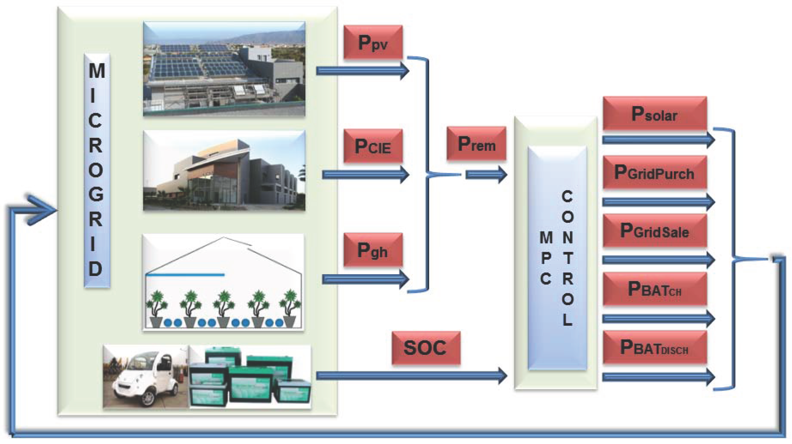All of these advantages are motivating an increased demand for microgrids in a variety of application areas such as campus environments, military operations, community/utility systems, as well as commercial and industrial markets [1]. An MG can provide optimal electricity distribution to consumers by implementing control strategies. Nowadays, the MG concept focuses primarily on the integration of distributed renewable energy sources, stationary storage batteries and methodologies for management and control, as is shown in [2,3,4,5,6].

In the literature, there are several MG methods and applications. In [7], the basic structure of an MG is presented, and a detailed discussion about MG control techniques is included. In [8], the authors review the latest documents related to the use of hybrid energy storage systems (HESS), which facilitate the introduction of renewable energy sources (RES) to MGs. A centralized and decentralized control architecture for microgrids and their possible applicability to serve the particular needs in microgrids are discussed in [9]. In [10], a summary of the available approaches is presented (system configuration, unit size and control and energy management) along with those currently being investigated for the optimal design of RES hybrid systems. A decentralized energy management system based on multi-agent systems theory employing fuzzy cognitive maps for its implementation is proposed in [11]. In [12], a framework for microgrid energy management, where each agent is seeking an optimal goal-directed action planning under power consumption, production and price uncertainties, is proposed, and the optimal scheduling strategy is achieved by using a robust optimization approach. A multi-objective optimization in order to minimize the energy cost and greenhouse gas emissions in a hybrid system including photovoltaic (PV), wind, battery storage and a micro gas turbine is proposed and implemented in [13]; furthermore, in [14], an optimal energy management of a standalone microgrid under different operational modes is studied; the system is tested under two different operational policies where microgrid power generation sources work with and without the battery storage system. Moreover, in [15], a control strategy for the integration of distributed storage systems in a photovoltaic and micro-current network is developed, which also includes varying loads. The proposed control allows the maximum use of photovoltaic energy under different MG operating conditions and provides a smooth transfer between network connection and isolation. In [16], a strategy based on model predictive control (MPC) is presented, where the optimization problem has been formulated as a mixed integer linear problem (MILP), the control algorithm for which has been validated in an MG located at the Center for Renewable Energy Sources and Saving, in Pikermi-Athens, Greece. On the other hand, in [17], an MPC algorithm in which the optimization problem has been formulated as a mixed-integer quadratic optimization (MIQP) has been applied to a microgrid located at the University of Seville, Spain. In [18], the authors compared the MPC techniques and the hysteresis band (HB) method in energy dispatch within a microgrid. The main difference between MPC and HB is that MPC guarantees optimality, while HB does not. The authors conclude that there is a dramatic reduction in the cost of operation using MPC techniques.

MG operating requirements are usually satisfied by a hierarchical control structure [19], where several authors have shared the idea of considering three levels associated with different time scales [20,21]. The primary level operates at a fast time scale, maintaining voltage and frequency stability during changes in the generation or load, or after switching to the island mode. The secondary level is responsible for ensuring that the voltage and frequency deviations are adjusted to zero after a load or generation change is produced within the microgrid. This tertiary control is used to control the power flow between the microgrid and the main grid and for optimal operation over large time scales [22].

The MG’s control loop performance can be improved when disturbance information is available. This can be done using a feedforward controller based on disturbance estimations, mainly of the demand and the available renewable energy. There are many methods for estimating energy demand, and these can be characterized by the prediction horizon length and the selected methodology. The prediction horizon may vary depending on the application and can be considered as a short-term forecast for predictions up to 60 min [23,24] or a long-term forecast for hourly, daily and monthly prediction values [25,26]. On the other hand, disturbances are usually represented as time-series structures mainly due to their stochastic behavior. Time-series models are one of the ways to estimate future energy demand values. These models are obtained using past data and are used to estimate future behavior along a prediction horizon. Time series models are based on the assumption that modeled data are autocorrelated and characterized by trends and seasonal variations. Thus, well-known autocorrelated models like autoregressive moving average (ARMA), autoregressive integrated moving average (ARIMA), autoregressive moving average with exogenous inputs (ARMAX) and autoregressive integrated moving average with exogenous inputs (ARIMAX) [27] can be used. Artificial neural networks (ANN) are a different approach for disturbance estimation when the design is training-based and no statistical conditions are assumed for the source data. Neural networks (NN) are widely accepted as a technology for predicting time series, offering an alternative way to solve complex problems [28]. Neural networks and ARIMA models are often compared in terms of forecasting capacity. As a tool for nonlinear system identification, the nonlinear autoregressive with exogenous inputs (NARX) network has been successfully applied to a number of real-world input/output modeling problems, such as biomedical time series modeling [29], communication network traffic prediction [30] and energy demand [31].

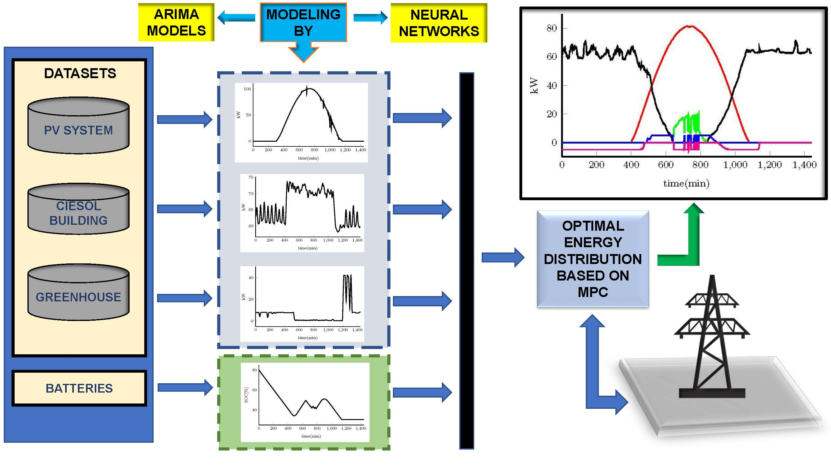
This paper studies the effect of using different prediction strategies in a closed-loop control framework for energy management in a real case study. Methods based on time series and neural network models are used for the photovoltaic panel energy production and the energy demand of the load systems (building and greenhouse). The models are identified using real data collected at a sampling time of 1 min during the years 2014 and 2015. The microgrid optimal energy management problem is formulated including binary variables in the constraints and solved as mixed integer quadratic programming (MIQP). In this way, the prediction models are utilized to provide a feedforward framework, and the usability of the predictions over different prediction horizons is discussed. It is important to emphasize that feedforward action effectiveness is directly connected to the predictions’ quality. Significant improvement is obtained for closed-loop system behavior compared to the case of constant future predictions. Moreover, controller performance is compared to an ideal case with perfect future predictions, and a discussion is carried out to evaluate the prediction methods.

The rest of the paper is organized as follows: in Section 2, the microgrid subsystems, the methods and the performance criteria used to model energy demand and electrical energy production are briefly shown, and the energy hub’s methodology is also presented; in Section 3, the results and discussions are shown, and finally, in Section 4, the conclusions are outlined.

2. Materials and Methods

The MG is composed of a photovoltaic system, an electric vehicle whose batteries can be used as an energy storage system (the use of the electric vehicle is not considered in this paper) and two load subsystems (a building and a greenhouse). Figure 1 shows the microgrid. Additionally, the microgrid is connected to the main grid, allowing the purchase and sale of energy when necessary.

2.1. Materials

2.1.1. The Greenhouse

The greenhouse studied in this paper is a multispan ’parral type’ greenhouse (see Figure 2), with a surface area of 877 m², oriented in a N-S direction.

The facilities are situated at the Cajamar Foundation experimental station,’Las Palmerillas’, in the El Ejido municipality, Almería, southeastern Spain [32]. The greenhouse has lateral and zenithal ventilation powered by independent AC motors, an aero-thermo heating system from hot water pipes fed with biomass, a CO₂ enrichment system created from burning biomass, shade nets, as well as water and nutrient feeding systems. It is equipped with measurement equipment for 52 variables and is designed to develop identification tests and to implement climate control, fertigation and electric power strategies. Furthermore, the greenhouse has energy demand sensors (SINEAX M 561) programmable with an RS-232 interface run on a computer with the appropriate software. In

Table 1. Sensory system installed in the greenhouse.

Variable	Model
Inside of the greenhouse
Temperature and humidity	HMP45a, Vaisala, Finland
Global radiation	MRG-1P, ITC, Almeria, España
CO2 concentration	UA-06, PRIVA B.V., De Lier, Holanda
Outside of the greenhouse
Temperature and humidity	HMP45a, Vaisala, Finland
Photosynthetic Active Radiation	PAR Lite
Global radiation	MRG-1P, ITC, Almeria, Spain
Wind speed	Model 12102, R. M. Young Company, Traverse City, Michigan, USA
Wind direction	D-034B-CA, Delta-T Devices Ltd, Cambridge, United Kingdom
CO${}_2$ concentration	ZFP–DZ, Siemens, Munich, Germany
Rain	WS 10 R, JUNG Electro Iberica S.A. Barcelona, Spain
Energy demand	SINEAX M 561 with 1, 2 resp. 3 analog outputs

, the variables measured and the model of the sensors used are detailed [33,34].

2.1.2. CIESOL Building

The CIESOL (’Centro de Investigación en Energía SOLar’) building is a solar energy research center, which is located inside the Campus of the University of Almería, in southeastern Spain (see Figure 3). It is distributed over two floors with a total surface area of $1071.92$ m², comprising: six offices, all with an easterly orientation and located on the ground floor (with the exception of the main office, situated on the upper floor); eight laboratories facing north (four located on the ground floor devoted to ’solar chemistry’; and the other four located on the upper floor: two for the ’Modeling and Automatic Control unit’ and the other two for the ’Evaluation of Solar Resources unit’); a plant where a high efficiency boiler and an absorption machine are located; and finally, the center’s employee rooms, such as the kitchen and toilets.

2.1.3. PV System

The PV system is made up of various sets located on-site at the University of Almería. One of these (see Figure 4) is located on the sloping roof of the CIESOL building and has the following characteristics: a total number of 4 modules linked in 3 sets of 14 panels/series, each with a unit capacity of 222 Wp/panel where the electrical energy produced is in the form of direct current at low voltage, then converted to alternating current through an inverter at a voltage of 230 V, forming a photovoltaic field of $9.324$ kWp.

Table 2. Summary for the PV module.

Module Type	A−222P
Peak Power Module (Wp)	222
Inverter model	CICLO 3000
Grid connection	3−phase
Electrical characteristics
Electricity power (Watts [W]$\pm 2\%$)	222 W
Number of cells in series	60
Current maximum power point (Imp [A])	7.44 A
High voltage power point (Vmp [V])	29.84 V
Short circuit current (Isc [A] )	7.96 A
Open circuit voltage (Voc [V])	37.20 V
Temperature coefficient of Isc ($\alpha$)	$2.30\frac{\mathrm{mA}}{\mathrm{C}}$
Temperature coefficient of Voc ($\beta$)	$127.20\frac{\mathrm{mV}}{\mathrm{C}}$
Maximum system voltage [V]	700 V

shows the summary and the main electrical characteristics of each module. The total set at the University of Almería that comprises the PV system considered in this paper forms a photovoltaic field that can reach 110 kWp.

2.1.4. Batteries

The bank of 6 batteries in the electric vehicle (Figure 5) that have been used in this MG is the Green Saver model with lead-acid silicone technology.

Table 3. Main battery features.

Type	SP125-12
Height	242 mm
Width	171 mm
Weight	$\mathrm{38,400}$ g
Voltage	12 V
Capacity	125 Ah

shows the summary for one battery.

2.1.5. Microgrid Controller

The MG uses a centralized controller [35] unit, which is responsible for correct process operation. The objective of this controller is to attend to the demand of the greenhouse and the CIESOL building, buying as little energy as possible from the main grid. The controller uses car batteries as energy storage units to optimize energy use during the day.

2.2. Methods

2.2.1. Hub Methodology

The methodology used in this paper to model the process has been presented in [36,37]. An energy hub is defined as the interface between energy production, consumers and the transmission line. From a system standpoint, a hub can be identified as a unit that provides the following features: (1) power input and output; (2) energy conversion; and (3) energy storage. Some of the main features of the hub are:

• Within energy hubs, losses occur only in the converter and storage elements.
• If not explicitly mentioned, unidirectional power flow from the inputs to the outputs of the converters is assumed.
• Power flow through converter devices is characterized by power and energy efficiency only; no other quantities are used.

The methodology is summarized as follows: a single converter converts, at time instant k, a generic r input flow $u_r^L\left(k\right)$ of a generic hub in a p output flow $y_p\left(k\right)$, where superscript L is associated with converter input flows. The input-output conversion is defined by the so-called coupling factor ${\gamma }_{p,r}^L$, which correspond to a converter steady-state conversion efficiency between the input and output flows:

$$y_p\left(k\right)={\gamma }_{p,r}^L{u}_r^L\left(k\right)$$

(1)

If we have several converters, it can be written as follows:

$$\underset{y_i\left(k\right)}{\underbrace{\left[\begin{array}{c}{y}_1\left(k\right)\\ ⋮\\ y_{n_p}\left(k\right)\end{array}\right]}}=\underset{{{\Gamma }}_i^L}{\underbrace{\left[\begin{array}{ccc}{\gamma }_{1,1}^L& \cdots & {\gamma }_{1,r}^L\\ ⋮& \ddots & ⋮\\ {\gamma }_{p,1}^L& \cdots & {\gamma }_{p,r}^L\end{array}\right]}}\underset{u_i^L}{\underbrace{\left[\begin{array}{c}{u}_1\left(k\right)\\ ⋮\\ u_{n_r}\left(k\right)\end{array}\right]}}$$

(2)

where ${{\Gamma }}_i^L$ is the converter coupling matrix.

From a discrete–time point of view, the internal storage state $x_{i,s}$ at sampling time $k+1$ depends on the state at the previous sample k and on the total exchanged flow ${\check{u}}_{i,s}^E\left(k\right)$ during the period $\Delta T$ ranging from k to $k+1$ sampling, where the values of steady state input-output flow are described by the relationship:

$${\check{u}}_{i,s}^E\left(k\right)=e_{i,s}\left(k\right)u_{i,s}^E\left(k\right)$$

(3)

where $e_{i,s}\left(k\right)$ is the efficiency of the $i,s$ interface charging/discharging hub, which describes the energy exchange between the system and the storage. This factor depends on the direction of flow exchanged as follows:

$$e_{i,s}=\begin{array}{c}\left\{\begin{array}{c}{e}_{i,s}^{+}if{u}_{i,s}^E\ge 0\left(charging\right)\hfill \\ e_{i,s}^{-}othercase\left(discharging\right)\hfill \end{array}\right.\hfill \end{array}$$

(4)

where $e_{i,s}^{+}$ and $e_{i,s}^{-}$ are the charging and discharging efficiency, respectively [38]. Assuming ${\check{u}}_{i,s}^E\left(k\right)$ remains constant during $\Delta T$:

$$x_{i,s}(k+1)=x_{i,s}\left(k\right)+{\int }_k^{k+1}{\check{u}}_{i,s}^E\left(t\right)dt=x_{i,s}\left(k\right)+{\check{u}}_{i,s}\left(k\right)\Delta T$$

(5)

If we consider several storage systems:

$$\begin{array}{c}\underset{x_i(k+1)}{\underbrace{\left[\begin{array}{c}{x}_{i,1}(k+1)\\ ⋮\\ x_{i,n_s}(k+1)\end{array}\right]}}=\underset{x_i\left(k\right)}{\underbrace{\left[\begin{array}{c}{x}_{i,1}\left(k\right)\\ ⋮\\ x_{i,n_s}\left(k\right)\end{array}\right]}}+\underset{{\mathsf{\Lambda }}_i^E\left(k\right)}{\underbrace{\left[\begin{array}{c}{e}_{i,1}\left(k\right)\\ \ddots \\ e_{i,n_s}\left(k\right)\end{array}\right]}}\underset{u_i^E\left(k\right)}{\underbrace{\left[\begin{array}{c}{\check{u}}_{i,1}^E\left(k\right)\\ ⋮\\ {\check{u}}_{i,n_s}^E\left(k\right)\end{array}\right]}}\hfill \end{array}$$

(6)

then, a single hub can be represented by the following condensed form:

$$\begin{array}{cc}\hfill x_i(k+1)& =x_i\left(k\right)+{\mathsf{\Lambda }}_i^E\left(k\right)u_i^E\left(k\right)\hfill \\ \hfill y_i\left(k\right)& ={{\Gamma }}_i^L{u}_i^L\left(k\right)\hfill \end{array}$$

(7)

2.2.2. Performance Criterion

When a certain method is used to estimate process variables, the differences between the estimated and real values can be employed to evaluate the method. Different statistical indexes can be utilized to compare the results of the forecasting models [25,39,40]. In this work, the mean square error (MSE), the root mean square error (RMSE), the mean absolute percentage error (MAPE) and the coefficient of determination $R^2$ will be used. The MSE is determined by:

$$MSE=\frac{1}{n}\sum _{k=1}^n{({\widehat{y}}_k-y_k)}^2$$

(8)

where n is the forecasting horizon, $y_k$ is the real signal at time k and $\widehat{y}$ is the estimated signal at time k. When a zero value is obtained for MSE, it means that the estimator ${\widehat{y}}_k$ predicts parameter observations $y_k$ with perfect accuracy.

RMSE is given by the square root of MSE:

$$RMSE=\sqrt{\frac{1}{n}\sum _{k=1}^n{({\widehat{y}}_k-y_k)}^2}$$

(9)

MAPE is defined as follows:

$$MAPE=\frac{100\%}{n}\sum _{k=1}^n\left|\frac{{\widehat{y}}_k-y_k}{y_k}\right|$$

(10)

The coefficient of determination $R^2$ provides a measurement of how well future outcomes are likely to be predicted by the forecasting method. It is calculated as follows:

$$R^2=\frac{{\sum }_{k=1}^N{({\widehat{y}}_k-\overline{y})}^2}{{\sum }_{k=1}^N{(y_k-\overline{y})}^2}$$

(11)

where $\overline{y}$ is the arithmetic mean value of the measured signal.

3. System Modeling and Control Algorithm

This section describes the modeling of the plant and the controller to be used. An MPC controller with linear constraints, whose formulation is detailed in [35], has been utilized in the MG control unit. To attempt the objectives described in Section 2.1.5, the following variable selection was defined.

3.1. Manipulated Variables

The MG input vector is defined according to:

$$\begin{array}{c}u=\left[\begin{array}{c}{u}_1\\ u_2\\ u_3\\ u_4\end{array}\right]=\left[\begin{array}{c}{P}_{GridPurch}\\ P_{GridSale}\\ P_{BA{T}_{CH}}\\ P_{BA{T}_{DISCH}}\end{array}\right]\end{array}$$

(12)

where $P_{GridPurch}$ and $P_{GridSale}$ are the purchase and sale of energy to the external network and $P_{BA{T}_{CH}}$ and $P_{BA{T}_{DISCH}}$ are the charging and discharging power of the batteries.

3.2. Disturbance Vector

The external disturbance to the MG is solar irradiation (measured in ${\mathrm{Wm}}^{-2}$) on the microgrid solar panels and directly affects the MG energy balance.

3.3. Controlled Variables

The controlled variables vector (system output vector) is defined as:

$$\begin{array}{c}y={\left[\begin{array}{c}{P}_{CIE}\\ P_{gh}\end{array}\right]}^T\end{array}$$

(13)

where $P_{CIE}$ is the energy demand of the CIESOL building (kW) and $P_{gh}$ is the greenhouse energy demand (kW).

3.4. Microgrid Model

The evolution of the microgrid state variable (the state of the batteries’ charge SOC_BAT) is described by the linear model:

$$\begin{array}{cc}\hfill SO{C}_{BAT}(k+1)& =SO{C}_{BAT}\left(k\right)+\frac{{\eta }_{BA{T}_{CH}}·P_{BA{T}_{CH}}\left(k\right)·T_s}{C_{BAT}}+\frac{{\eta }_{BA{T}_{DISCH}}·P_{BA{T}_{DISCH}}\left(k\right)·T_s}{C_{BAT}}\hfill \end{array}$$

(14)

where ${\eta }_{BA{T}_{CH}}$ and ${\eta }_{BA{T}_{DISCH}}$ are the charging and discharging efficiency of the battery, respectively. $T_s$ is the sample time, and $C_{BAT}$ is the battery capacity.

Net power balance ($P_{rem}\left(k\right)$) within MG is considered. $P_{pv}={\eta }_{solar}Irrad\left(k\right)$ and $P_{solar}=P_{pv}$. $P_{pv}$, ${\eta }_{solar}$ and $Irrad\left(k\right)$ are, respectively, the energy production of the PV panels, the solar energy conversion efficiency and the solar irradiation that acts as a disturbance. Figure 6 shows the control diagram.

Therefore, the MG can be modeled as a single hub in a condensed form as:

$$\begin{array}{cc}\hfill x(k+1)& =Ax\left(k\right)+\mathsf{\Lambda }u\left(k\right)\hfill \\ \hfill y\left(k\right)& ={\Gamma }u\left(k\right)+DIrrad\left(k\right)\hfill \end{array}$$

(15)

where:

$$\begin{array}{ccc}\hfill A& =& \left[1\right]\hfill \end{array}$$

(16)

$$\begin{array}{ccc}\hfill \mathsf{\Lambda }& =& \left[00\frac{{\eta }_{BA{T}_{CH}}·T_s}{C_{BAT}}\frac{{\eta }_{BA{T}_{DISCH}}·T_s}{C_{BAT}}\right]\hfill \end{array}$$

(17)

$$\begin{array}{ccc}\hfill {\Gamma }& =& [1-1-1-1]\hfill \end{array}$$

(18)

$$\begin{array}{ccc}\hfill D& =& \left[{\eta }_{solar}\right]\hfill \end{array}$$

(19)

3.5. Controller

The controller is designed to perform the energy management of the microgrid under energy changes during the generation or loads and managing the use of energy storage system. The MPC cost function is given by:

$$\begin{array}{cc}\hfill J& =\sum _{l=0}^{N_p-1}(\tilde{u}{(k+l)}^T{Q}_u\tilde{u}(k+l)+f^T\tilde{u}(k+l))+\sum _{l=0}^{N_p-1}{(\tilde{x}(k+l)-{\tilde{x}}_{ref}(k+l))}^T{Q}_x(\tilde{x}(k+l)-{\tilde{x}}_{ref}(k+l))\hfill \end{array}$$

(20)

s.t.

$$\begin{array}{ccc}\hfill \underline{x}& \le & \tilde{x}(k+l+1)\le \overline{x}\hfill \end{array}$$

(21)

$$\begin{array}{ccc}\hfill \underline{u}& \le & \tilde{u}(k+l+1)\le \overline{u}\hfill \end{array}$$

(22)

$$\begin{array}{ccc}\hfill \tilde{y}(k+l)& =& P_{CIE}\left(k\right)+P_{gh}\left(k\right)\hfill \end{array}$$

(23)

where $l=0,\cdots ,N_p-1$, $Q_u$ and $Q_x$ are positive definite weighting matrices, f is a linear function and $N_p$ is the prediction horizon. Regarding the notation “$\tilde{a}$” over variables, this is used to denote variables over the prediction horizon; $\underline{a}$ and $\overline{a}$ denote the minimum and maximum allowed values, respectively. The first term of the objective function (20) has been used for the management of renewable sources and the purchase/sale of energy from the grid. The weights $Q_u$ and f are tuned to minimize the use of the network and the storage system. In the second term, $Q_x$ is tuned to maintain the storage load around $50\%$ allowing deviations from this value when there is a need to store more energy and use the stored energy; the minimum charge state allowed in the batteries is $30\%$. An initial state in the batteries of $80\%$ has been considered.

To ensure the proper use of the renewable energy sources, to manage the purchase and sale of electricity to the external network and to use the storage to minimize oscillations between production and demand, binary variables are introduced to the formula as constraints in the following way:

$${\delta }_{GridPurch}\left(k\right)=\begin{array}{c}\left\{\begin{array}{c}1,P_{GridPurch}\left(k\right)>0\hfill \\ 0,P_{GridPurch}\left(k\right)=0\hfill \end{array}\right.\hfill \end{array}$$

(24)

$${\delta }_{GridSale}\left(k\right)=\begin{array}{c}\left\{\begin{array}{c}1,P_{GridSale}\left(k\right)>0\hfill \\ 0,P_{GridSale}\left(k\right)=0\hfill \end{array}\right.\hfill \end{array}$$

(25)

$${\delta }_{GridPurch}\left(k\right)+{\delta }_{GridSale}\left(k\right)=1$$

(26)

$${\delta }_{BA{T}_{CH}}\left(k\right)=\begin{array}{c}\left\{\begin{array}{c}1,P_{BA{T}_{CH}}\left(k\right)>0\hfill \\ 0,P_{BA{T}_{CH}}\left(k\right)=0\hfill \end{array}\right.\hfill \end{array}$$

(27)

$${\delta }_{BA{T}_{DISCH}}\left(k\right)=\begin{array}{c}\left\{\begin{array}{c}1,P_{BA{T}_{DISCH}}\left(k\right)<0\hfill \\ 0,P_{BA{T}_{DISCH}}\left(k\right)=0\hfill \end{array}\right.\hfill \end{array}$$

(28)

$${\delta }_{BA{T}_{CH}}\left(k\right)+{\delta }_{BA{T}_{DISCH}}\left(k\right)=1$$

(29)

The state space formulation of the hub has been transformed into the mixed logical dynamic (MLD) formulation considering concepts of propositional calculus and integer linear programming, as shown in [41]. This formulation makes it possible to include binary variables introduced in a discrete-time dynamic system in order to describe the evolution of the system’s continuous and logic signals in a unified model.

The conditions $P_j\left(k\right)>0$ in Equations (24), (25) and (27) and condition $P_{BA{T}_{DISCH}}<0$ in Equation (28) can be associated with a binary variable ${\delta }_j$ for $j=\{GridPurch,GridSale,BA{T}_{CH}\}$ and ${\delta }_{BA{T}_{DISCH}}$, respectively, such that:

$$\begin{array}{c}\left[P_j\left(k\right)>0\right]\to \left[{\delta }_j\left(k\right)=1\right]\\ \left[P_{BA{T}_{DISCH}}<0\right]\to \left[{\delta }_{BA{T}_{DISCH}}\left(k\right)=1\right]\end{array}$$

(30)

Equation (30) can be expressed by the inequalities:

$$\begin{array}{c}(M+ϵ){\delta }_j\left(k\right)-P_j{\delta }_j\left(k\right)>0\\ (m+ϵ){\delta }_{BA{T}_{DISCH}}\left(k\right)-P_{BA{T}_{DISCH}}{\delta }_{BA{T}_{DISCH}}\left(k\right)<0\end{array}$$

(31)

where

$$\begin{array}{c}m=min{P}_{BA{T}_{DISCH}}\left(k\right)\hfill \\ M=max{P}_j\left(k\right)\hfill \end{array}$$

(32)

and $ϵ$ is a small tolerance (typically the machine precision).

In Equation (24), $P_{GridPurch}\left(k\right)>0$ gives ${\delta }_{GridPurch}\left(k\right)=1$, which means that the energy is purchased from the grid and therefore the weight is used on the purchase value, in (25); on the other hand $P_{GridSale}\left(k\right)>0$ results in ${\delta }_{GridSale}\left(k\right)=1$, which means that the energy is sold to the grid, and therefore, the weight is used on the sale value. Analogous analysis is performed for Equations (27) and (28). Furthermore, Equations (26) and (29) are associated with the exclusive sum (exclusive or), such that:

$$\begin{array}{c}\left[P_{GridPurch}\left(k\right)\oplus P_{GridSale}\left(k\right)\right]\\ \left[P_{BA{T}_{CH}}\left(k\right)\oplus P_{BA{T}_{DISCH}}\left(k\right)\right]\end{array}$$

(33)

This means that only one action can be performed once, buying or selling energy and charging or discharging battery energy; moreover, doing neither is not possible.

4. Simulation Results and Discussion

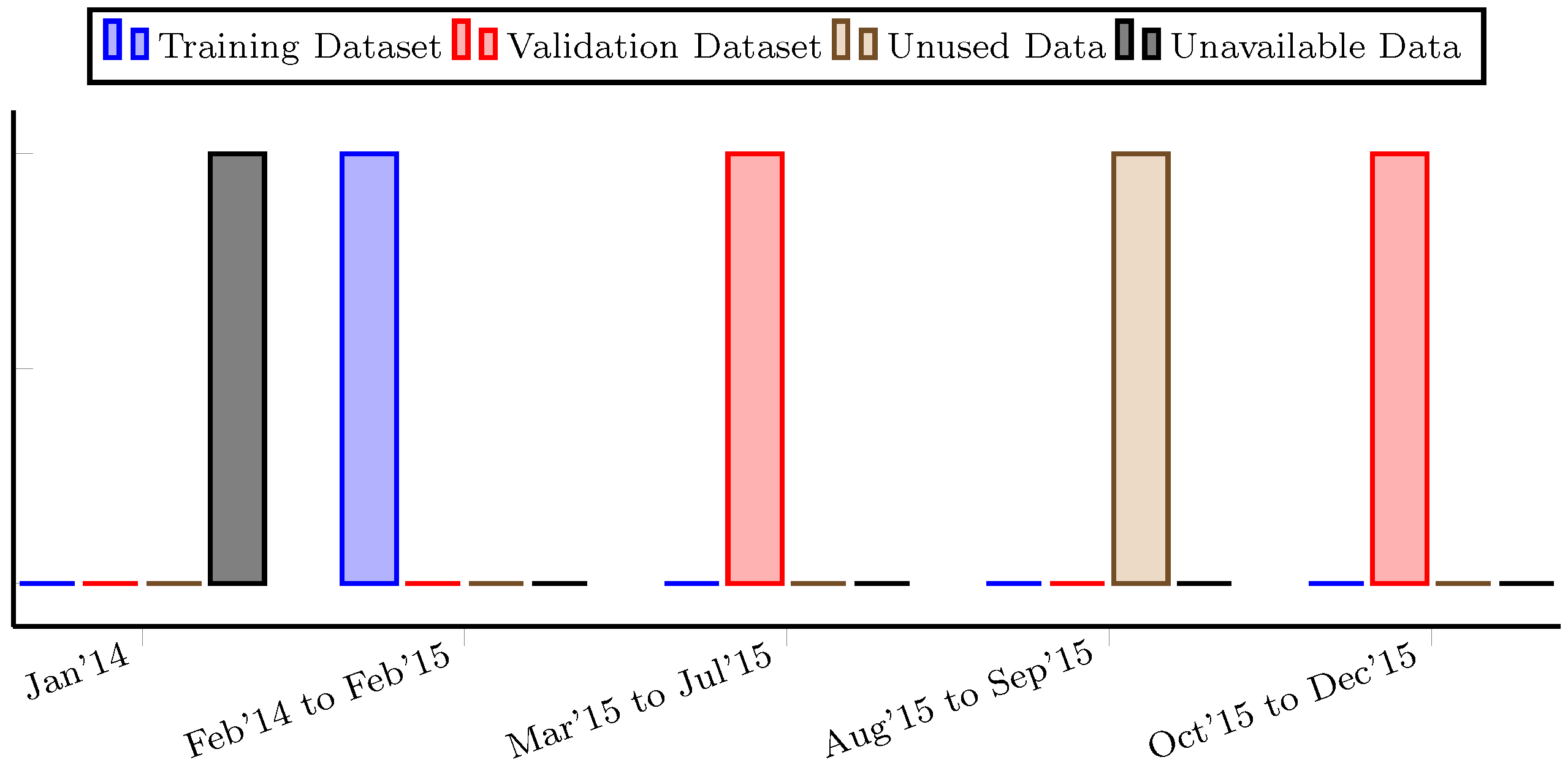
This section presents the results obtained from applying the control and prediction methods. As already mentioned, the analysis mainly focuses on load prediction, which has been executed with forecasting steps given minute by minute. The energy demand and production were previously filtered using the Savitzky–Golay filter [42] in order to preserve initial distribution characteristics such as the relative maximum and minimum, as well as the width of the peaks. Data from 2014 have been used to identify the models and during different days of the year 2015 have been used for validation (see Figure 7). Different scenarios are presented using the proposed controller in order to realize optimal energy distribution and to observe the contribution made by the prediction models on two different significant days.

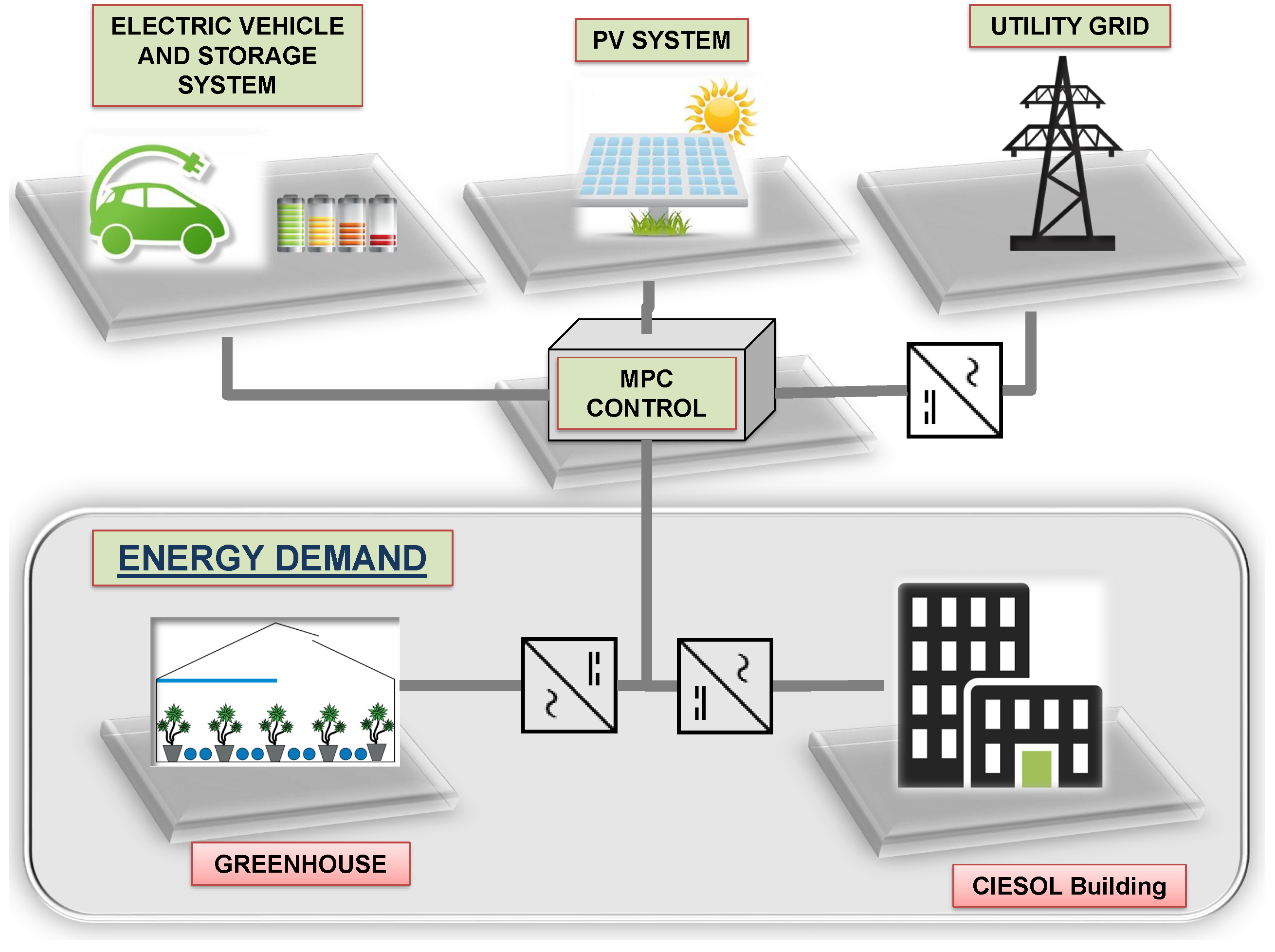
4.1. CIESOL Building and PV System

Two models for each system were proposed. Firstly, we compared several combinations of the autoregressive moving average (ARMA) models using the final prediction error (FPE) [43]; these models were based on historical energy demand and energy production data. The data used to identify these models were chosen from data collected over the year 2014. The ARMA model for a single-output time series is given by the following equation:

$$A\left(z^{-1}\right)y\left(k\right)=C\left(z^{-1}\right)e\left(k\right)$$

(34)

where $y\left(k\right)$ is the system output and $e\left(k\right)$ is the model error. The ARMA structure reduces to the autoregressive (AR) structure for $C\left(z^{-1}\right)=1$ as is mentioned in [43].

The discrete-time polynomials obtained for the CIESOL building energy demand (A1) and for the energy production of the PV system (A2) are detailed in Appendix A.

Additionally, for the same periods and minimizing the MSE, we evaluated several combinations of the NAR neural network multilayer perceptron using the Levenberg–Marquardt algorithm. These combinations included networks with different numbers of hidden layers, different numbers of units in each layer and different types of transfer functions. The chosen configuration consisted of one hidden layer with 11 and 10 neurons for CIESOL and the PV system, respectively, and a hyperbolic tangent sigmoid transfer function within this layer, defined by the equation:

$$f\left(n\right)=\frac{1-e^{-n}}{1+e^{-n}}$$

(35)

where n is the weighted input of the hidden layer and $f\left(n\right)$ is the output of the hidden layer. For the output layer, a log-sigmoid transfer function was selected (36), and eight and six neurons for CIESOL and the PV system were used, respectively.

$$f\left(n\right)=\frac{1}{1+e^{-n}}$$

(36)

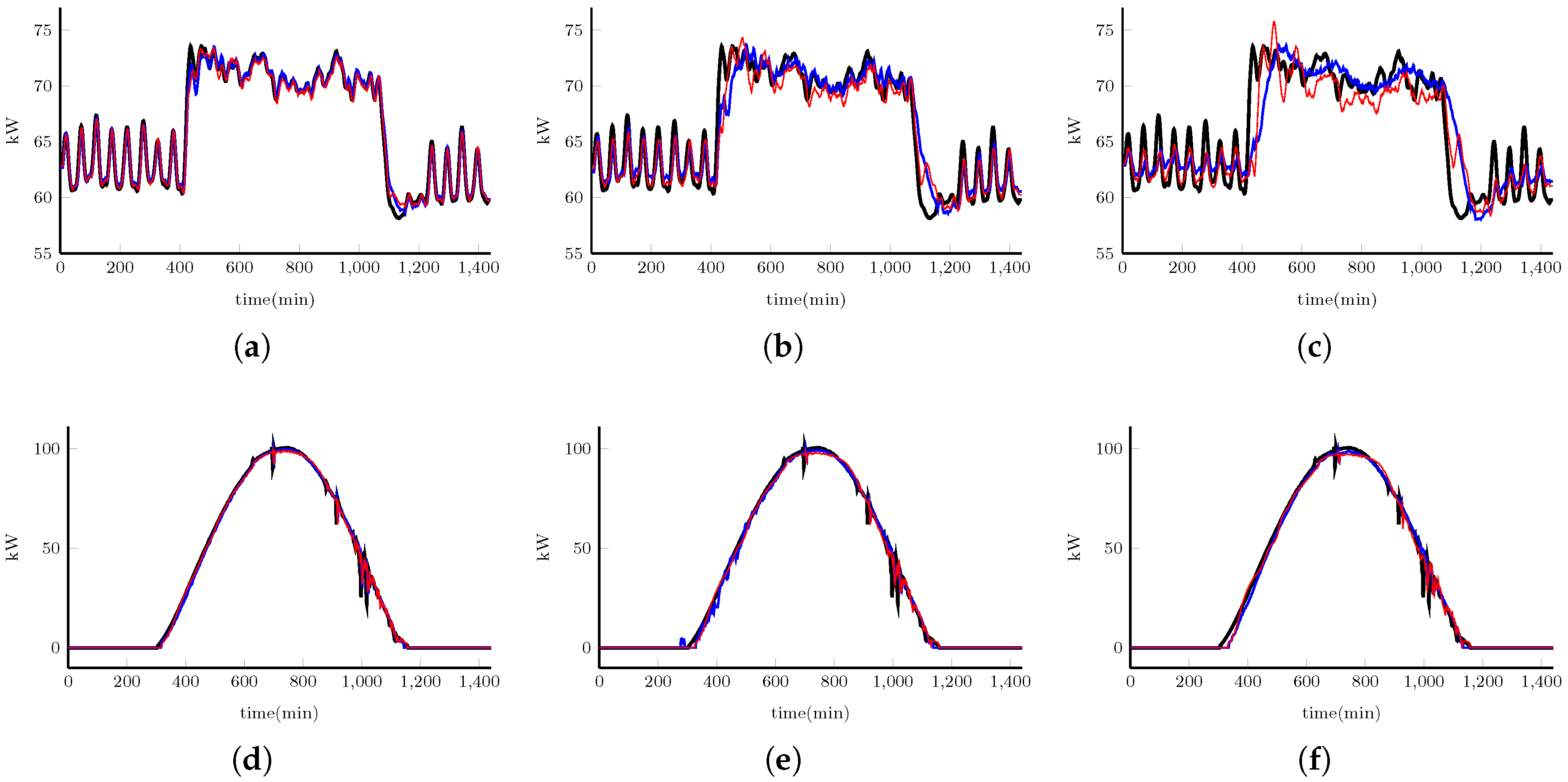
In order to evaluate prediction accuracy, these models were evaluated for predictions with 5, 10 and 15 horizon samples. Figure 8 and

Table 4. Performance indexes for the prediction model of the CIESOL building and the PV system with 5-, 10- and 15-sample prediction horizons.

Subsystem	Indexes	5 Samples		10 Samples		15 Samples
		ARMA	NN	ARMA	NN	ARMA	NN
	MSE	0.313	0.291	2.174	2.002	5.893	4.949
CIESOL	RMSE	0.559	0.539	1.147	1.415	2.427	2.224
Building	MAPE	0.594	0.582	1.601	1.481	2.587	2.332
	$R^2$	0.986	0.987	0.908	0.915	0.751	0.791
	MSE	3.653	3.524	5.364	5.010	6.6523	6.468
PV	RMSE	1.911	1.877	2.316	2.238	2.554	2.543
system	MAPE	8.576	8.115	12.126	11.213	15.189	13.448
	$R^2$	0.997	0.997	0.996	0.996	0.995	0.995

show the obtained results.

For the CIESOL building, one can observe that both models (ARMA and NN) produced good performance; however, it can also be observed that the NN model better approximated the peak demand and showed better results for all sample horizons. One can see that the neural networks method is able to capture sudden changes, whereas the ARMA method only follows the trend. The lower MSE, RMSE and MAPE values of the NN model for all horizons show that it is better than the ARMA model; furthermore, the $R^2$ is the square of the sample correlation coefficient between the real samples, and their predicted values-values close to one are desired. The resulting $R^2$ values for this analysis are satisfactory, with the NN model presenting higher values than the ARMA model. However, for a 15-sample prediction horizon, one can observe that a substantial change exists for that of the 10-sample prediction horizon in both models; that is, both models are able to follow the trend, but the energy demand peaks have not been captured.

Conversely, for the photovoltaic system, the best results derived from the neural network model for all sample horizons. Moreover, one can see that the two models produce a small predicted signal delay when clouds are passing. Nevertheless, the neural network model provides the best performance according to Table 4 with smaller differences compared to the ARMA model, in which the absolute percentage error measurement shows that the best forecasting accuracy is provided by the NN model (this does not exceed $13.5\%$ for the 15-sample horizon). One can also observe that, when there is a substantial change in radiation, both 15-sample prediction horizon models take longer to follow the process dynamics. In contrast, there is no great change in the 10-sample prediction horizon.

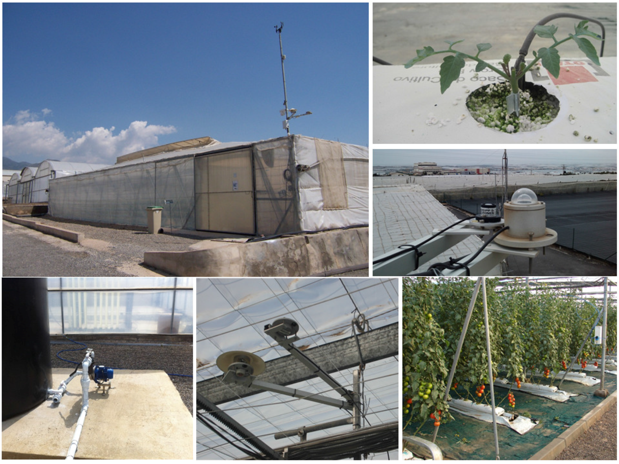
4.2. The Greenhouse

The energy demand has been considered as a MISO (multi-input single-output) system, where inside temperature, $v_1\left(k\right)$, outside temperature, $v_2\left(k\right)$, inside relative humidity, $v_3\left(k\right)$, global radiation, $v_4\left(k\right)$, blower, $u_1\left(k\right)$, pump heating, $u_2\left(k\right)$, zenithal ventilation, $u_3\left(k\right)$, and lateral ventilation, $u_4\left(k\right)$, were the input variables, and energy demand, $y\left(k\right)$, was the output variable. All greenhouse variables were measured with a sampling period of 1 min. In order to calculate future predictions, the future inputs were considered as known; however, these inputs can be estimated by other prediction models. A model based on Bayesian networks was presented in [34] considering these variables, where the energy demand was classified into four classes. One of the main problems when considering energy demand classes is that information is lost about the real demand values.

In this paper, the real value of the energy demanded is represented; meaning energy information is not lost when defining it within classes. It has been observed that energy demand behavior in the greenhouse was that of low energy demand during the spring-summer and high energy demand during the autumn-winter. This is because during the spring-summer, there is no crop, and the cultivation period occurs during the autumn-winter, when a controlled temperature inside the greenhouse has to be maintained using different heating systems due to the low overnight temperatures. Accordingly, four models were proposed, an autoregressive with external input (ARX) model and one based on neural networks for the autumn-winter season, as well as an ARX model and an NN model for the spring-summer season. To identify the spring-summer models, we considered data from 22 February 2014–21 September 2014. For the autumn-winter season, data from 22 September 2014–21 February 2015 were chosen.

Several ARX models were performed. An ARX model was observed as follows:

$$\begin{array}{cc}\hfill A\left(z^{-1}\right)y\left(k\right)& =\sum _{i=1}^{{\alpha }_1,{\beta }_1}{z}^{-d_{B_i}}{B}_i\left(z^{-1}\right)u_i\left(k\right)+\sum _{i=1}^{{\alpha }_2,{\beta }_2}{z}^{-d_{D_i}}{D}_i\left(z^{-1}\right)v_i\left(k\right)+\frac{ϵ\left(k\right)}{\Delta }\hfill \end{array}$$

(37)

Using Akaike’s Information Criterion (AIC) [44], better dynamic behavior adjustment was presented to the real system, where ${\alpha }_1=4$ and ${\alpha }_2=5$ for the autumn-winter model and ${\beta }_1=6$ and ${\beta }_2=10$ for the spring-summer model were used, respectively.

The discrete-time polynomials obtained for the autumn-winter season (A3) and for the spring-summer season (A4) are shown in Appendix A.

On the other hand, to find the optimal network architecture, several combinations of NARX neural network multilayer perceptron were evaluated using the Levenberg–Marquardt algorithm minimizing the MSE. These combinations included networks with different numbers of hidden layers, different numbers of units in each layer and different types of transfer functions.

A configuration was chosen consisting of a hidden layer with 11 and 12 neurons for the autumn-winter season and spring-summer season, respectively, along with a hyperbolic tangent sigmoid transfer function in this layer, defined by (35). For the output layer, a linear transfer function was selected with eight neurons for the autumn-winter season and eight neurons for the spring-summer season.

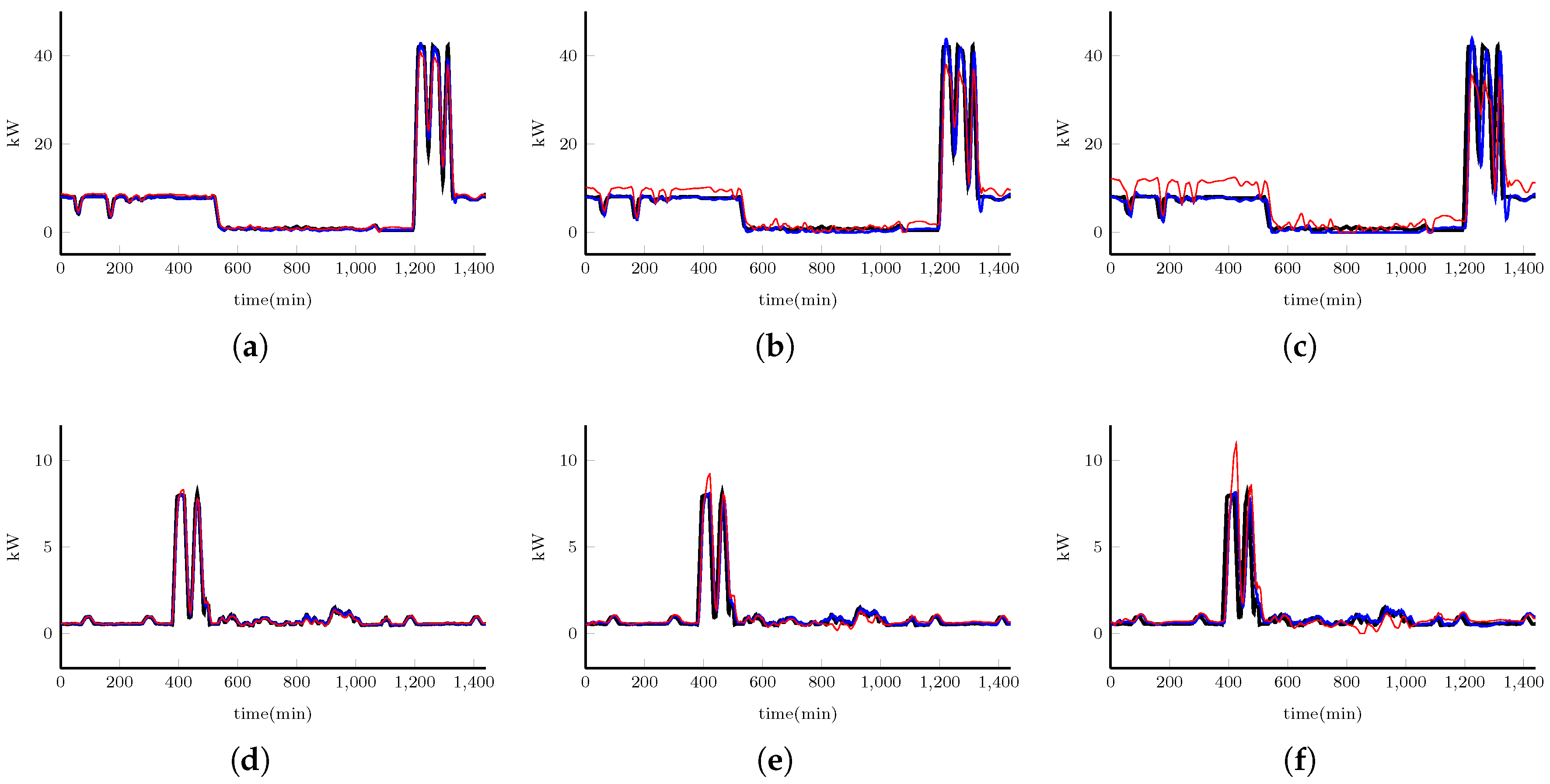
Figure 9 shows the one-day forecasting results during the autumn-winter and the spring-summer season of 2015 using a prediction horizon of 5, 10 and 15 samples. The results are summarized in

Table 5. Performance indexes for the greenhouse prediction model with 5-, 10- and 15-sample prediction horizons.

Season	Indexes	5-Samples		10-Samples		15-Samples
		ARX	NN	ARX	NN	ARX	NN
autumn-winter	MSE	0.797	1.126	6.655	7.639	19.305	21.101
	RMSE	0.893	1.061	2.579	2.764	4.393	4.593
	MAPE	11.334	23.235	34.146	65.026	48.953	106.51
	$R^2$	0.990	0.986	0.919	0.907	0.767	0.745
spring-summer	MSE	0.028	0.028	0.215	0.259	0.661	1.032
	RMSE	0.167	0.170	0.463	0.509	0.813	1.016
	MAPE	5.344	8.231	13.98	22.081	26.098	40.723
	$R^2$	0.985	0.985	0.890	0.867	0.663	0.473

. The changes in energy demand during the autumn-winter season were more abrupt than in the spring-summer season, meaning the models obtained for the autumn-winter season had a greater prediction error compared to the spring-summer season models.

The resulting values of $R^2$ for this analysis are satisfactory for both models with a 5- and 10-sample prediction horizon; however, one can see that for a 15-sample prediction horizon, the coefficient $R^2$ is below 0.7 for the spring-summer season. For the autumn-winter season, the ARX model values are $0.990$, $0.919$ and $0.767$, compared to the NN model values of $0.986$, $0.907$ and $0.745$ for the 5-, 10- and 15-sample prediction horizons, respectively. Furthermore, for the spring-summer season, the ARX model values are $0.985$, $0.890$ and $0.663$ against the NN model values of $0.985$, $0.867$ and $0.473$ for the 5-, 10- and 15-sample prediction horizons, respectively. Consequently, the ARX models give better results than the NN models for both seasons.

4.3. An Optimal Distribution Using the Proposed Controller

The predictive controller previously presented in Section 3 has been applied to the MG. The results presented in this section were obtained considering the following conditions:

• The simulation used real data collected for a sunny day and a day with passing clouds.
• Three similar sets of batteries that can reach a total capacity of $C=20$ kWh and a charging ${\eta }_{BA{T}_{CH}}=0.8$ and discharging ${\eta }_{BA{T}_{DISCH}}=0.7$ efficiency, respectively, and 10 similar greenhouses, such as those presented in the materials section, were considered.
• The cost involved in the degradation of the batteries has been considered constant. In addition, the maintenance cost of the photovoltaic system has not been considered.
• It is considered to maintain the state of charge of batteries at $50\%$ throughout the day.
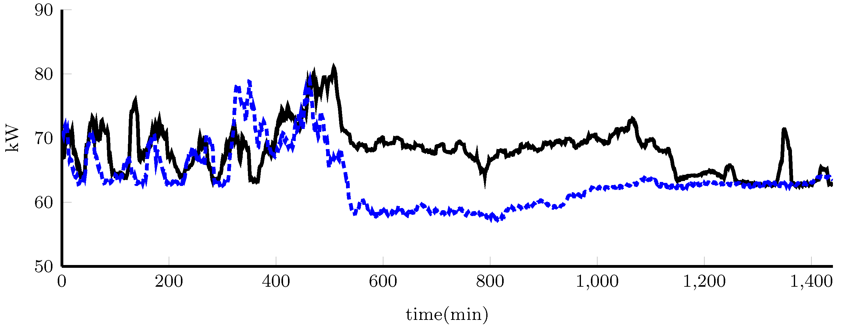
• Figure 10 shows the energy demand profiles for both types of day.
• The cost function weights (20) were adjusted using simulations.
• The proposed controller was applied to the microgrid. The aim of the controller is to perform the energy management of the microgrid during changes in generation or loads. The controller was implemented in MATLAB [45] using the YALMIP [46] toolbox and the CPLEX [47] solver.
• The simulations were performed using a control horizon of $N_c=5$ samples and a prediction horizon, which varied from 6 to 15, ($N_p=6,7,\cdots ,15$).

In order to verify the contributions of the models presented in Section 4.1 and Section 4.2 to the predictive control techniques, three different scenarios have been considered in this paper:

(i)

Perfect information: Scenario 1 is performed assuming that the real data of demand ($P_{CIE}$ and $P_{gh}$) and energy production ($P_{pv}$) are known.

(ii)

Imperfect information: Scenario 2 is performed using the best forecasting models of demand (the NN model for $P_{CIE}$ and the ARX model $P_{gh}$) and energy production (the NN model for $P_{pv}$).

(iii)

No Information: Scenario 3 is performed assuming that future values are not known and predictive models for demand ($P_{CIE}$ and $P_{gh}$) and energy production ($P_{pv}$) are not used. This means that the predictions are considered constant along the prediction horizon.

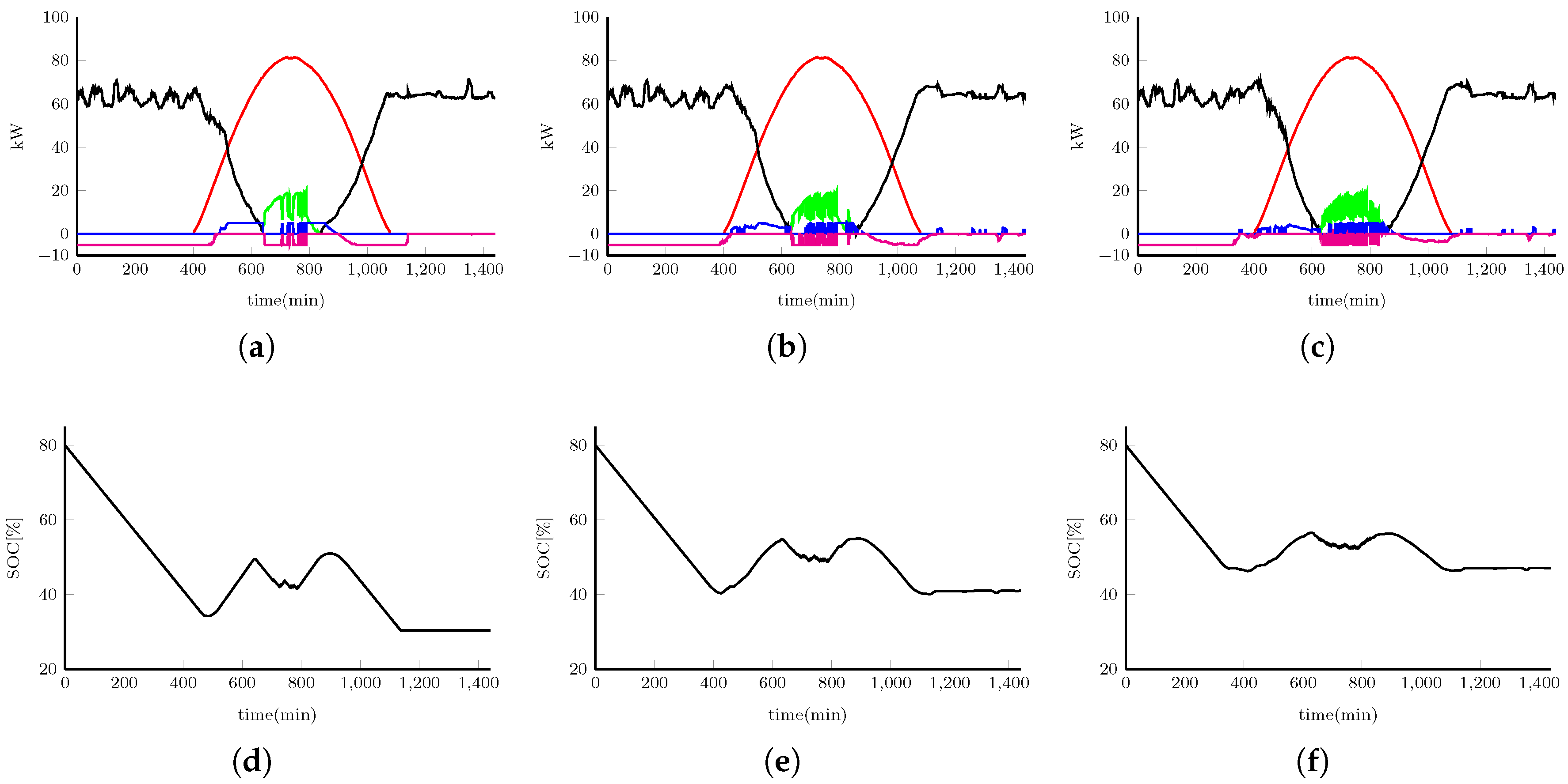
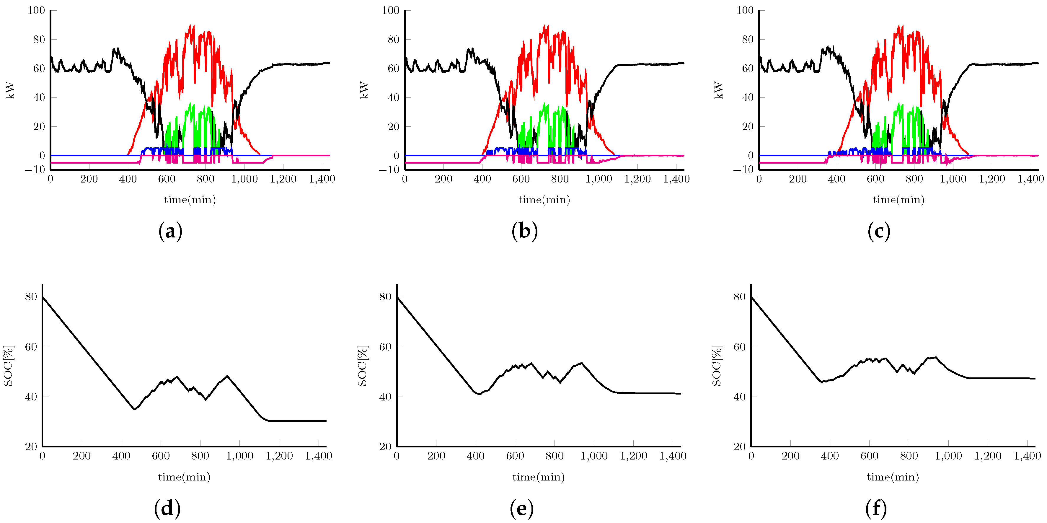
Figure 11 and Figure 12 show the behavior simulations for the electrical energy distribution and the SOC in Scenario 2 on a sunny day and a day with passing clouds for a prediction horizon of 6, 10 and 15 samples, respectively. One can see that, as the prediction horizon grows, there are larger fluctuations in the variables $P_{Gri{d}_{Purch}}$, $P_{Gri{d}_{Sale}}$, $P_{BA{T}_{CH}}$ and $P_{BA{T}_{DISCH}}$, causing greater effort from the batteries and resulting in more energy being bought and less energy being sold. Figure 11d–f and Figure 12d–f show how the SOC of the batteries tries to stay around its reference for a sunny day and for the day with passing clouds, respectively. Furthermore, one can observe that the lower prediction horizon has a greater variation range during the day. As can be seen, the three scenarios for both days have been realized trying to maintain the same level ($50\%$) of the SOC throughout the day and considering the design of the controller; this has been done with the aim of observing the contribution of prediction models. However, depending on the controller design, the results may vary. In the design of the controller, it could be required that at the end of the day, the SOC tries to maintain a different reference level.

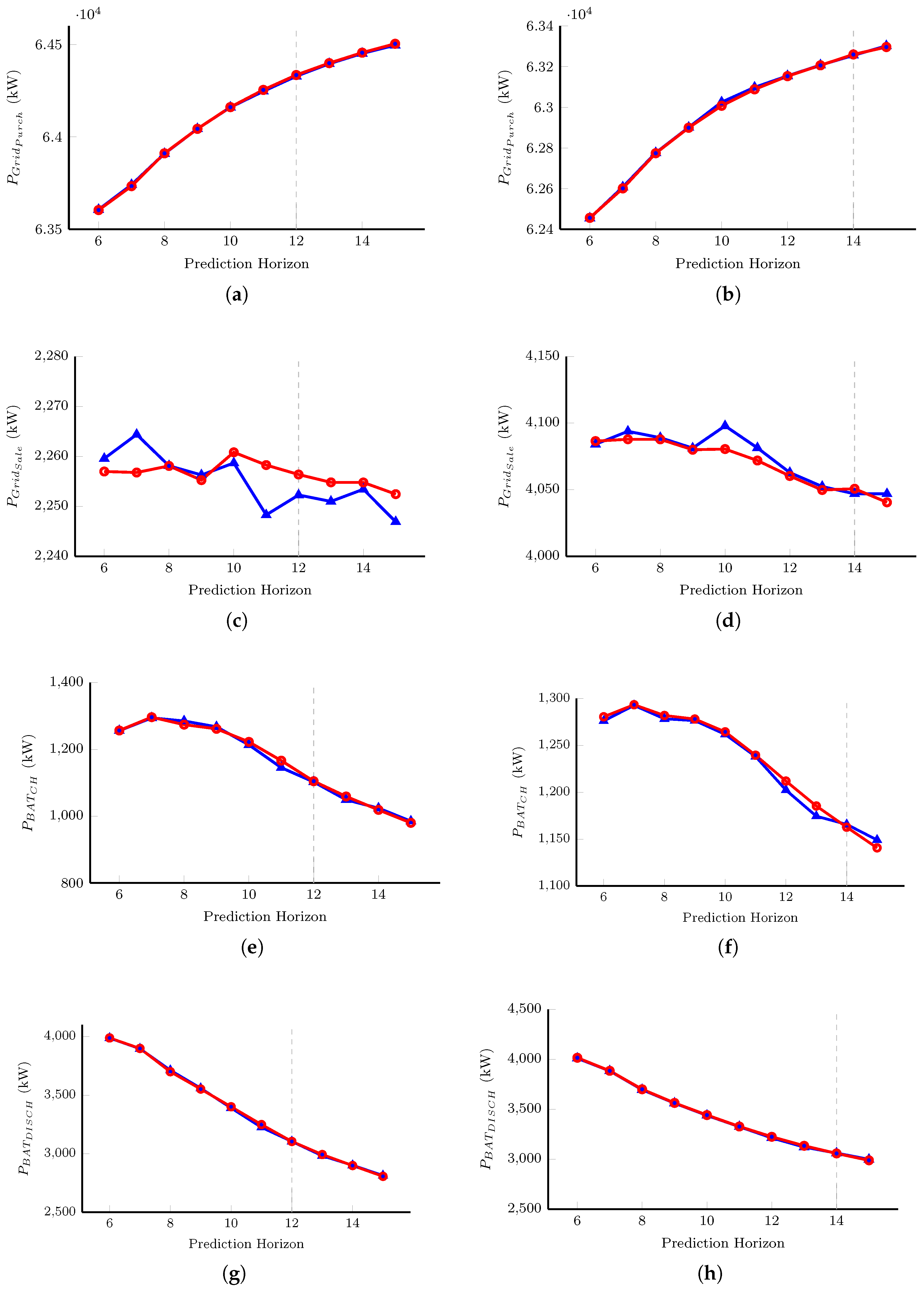
In addition, small differences can be observed by considering the total sum of each manipulated variable during the day (see

Table A1. Energy (kW) distributed for prediction horizons from 6–15 min with separation intervals of 1 min on a sunny day.

⧫	Total	Prediction Horizon (Min)
	Energy	6	7	8	9	10	11	12	13	14	15
	$P_{solar}$	34,021	34,021	34,021	34,021	34,020	34,021	34,021	34,021	34,021	34,021
	$P_{GridPurch}$	63,609	63,737	63,907	64,058	64,153	64,248	64,333	64,398	64,457	64,506
1	$P_{GridSale}$	2261	2260.6	2256.2	2269.9	2250.8	2249.5	2257.1	2255	2256.3	2256.5
	$P_{BA{T}_{CH}}$	1250	1294.6	1287.5	1265.5	1210.7	1150.5	1101.8	1062.1	1017.7	980.2
	$P_{BA{T}_{DISCH}}$	3980.1	3895.9	3714.6	3555.8	3386.9	3230.3	3103.7	2997.2	2894.9	2808.7
	$P_{solar}$	34,021	34,021	34,021	34,021	34,021	34,021	34,021	34,021	34,021	34,021
	$P_{GridPurch}$	63,606	63,741	63,909	64,044	64,160	64,247	64,328	64,396	64,451	64,496
2	$P_{GridSale}$	2259.6	2264.4	2258.1	2256.3	2258.7	2248.3	2252.3	2251	2253.4	2246.9
	$P_{BA{T}_{CH}}$	1256.8	1295.3	1285.8	1268.4	1214.3	1145.8	1103	1049.5	1024.2	985.2
	$P_{BA{T}_{DISCH}}$	3987.8	3896.7	3712.6	3559.1	3390.9	3225.4	3105	2982.9	2901.5	2814.3
	$P_{solar}$	34,021	34,021	34,021	34,021	34,021	34,021	34,021	34,021	34,021	34,021
	$P_{GridPurch}$	63,604	63,733	63,911	64,043	64,161	64,254	64,335	64,399	64,456	64,504
3	$P_{GridSale}$	2257	2256.8	2258.1	2255.3	2260.8	2258.3	2256.4	2254.8	2254.8	2252.4
	$P_{BA{T}_{CH}}$	1257.4	1297.3	1275	1262.4	1223.2	1166.9	1105.2	1059.4	1019.1	980.2
	$P_{BA{T}_{DISCH}}$	3988.5	3899	3700.2	3552.3	3401.1	3249.2	3104.9	2993.3	2899.1	2807.1

and

Table A2. Energy (kW) distributed for prediction horizons from 6–15 min with separation intervals of 1 min on a day with passing clouds.

⧫	Total	Prediction Horizon (Min)
	Energy	6	7	8	9	10	11	12	13	14	15
	$P_{solar}$	30,291	30,291	30,291	30,291	30,291	30,291	30,291	30,291	30,291	30,291
	$P_{GridPurch}$	62,453	62,615	62,781	62,923	63,024	63,111	63,175	63,222	63,265	63,299
1	$P_{GridSale}$	4082.5	4101.2	4092.4	4102.3	4094	4092.8	4081.4	4065.3	4054.2	4042.3
	$P_{BA{T}_{CH}}$	1275.3	1287.6	1268.8	1267.8	1245.4	1224.7	1197.4	1174.4	1154.2	1136.6
	$P_{BA{T}_{DISCH}}$	4008.9	3877.6	3684.7	3551	3419.9	3310.3	3207.9	3121.8	3047.9	2984.1
	$P_{solar}$	30,291	30,291	30,291	30,291	30,291	30,291	30,291	30,291	30,291	30,291
	$P_{GridPurch}$	62,455	62,607	62,776	62,901	63,025	63,098	63,154	63,208	63,256	63,302
2	$P_{GridSale}$	4084.1	4093.8	4089.1	4081.2	4097.9	4081.4	4062.8	4052.4	4046.9	4046.9
	$P_{BA{T}_{CH}}$	1276.1	1292.7	1278.4	1276.5	1261.8	1238.2	1202.4	1174.5	1165.7	1149.1
	$P_{BA{T}_{DISCH}}$	4009.8	3883.5	3695.7	3560.9	3438.6	3325.8	3213.7	3122	3061.1	2998.4
	$P_{solar}$	30,291	30,291	30,291	30,291	30,291	30,291	30,291	30,291	30,291	30,291
	$P_{GridPurch}$	62,456	62,601	62,774	62,900	63,008	63,088	63,153	63,206	63,260	63,296
3	$P_{GridSale}$	4086.5	4087.9	4087.8	4080	4080.5	4071.9	4060.3	4049.8	4050.7	4040.5
	$P_{BA{T}_{CH}}$	1280.6	1293.4	1282	1278.2	1264.5	1239.6	1212	1185.4	1162.8	1140.7
	$P_{BA{T}_{DISCH}}$	4015	3884.3	3699.8	3562.8	3441.6	3327.3	3224.6	3134.4	3057.8	2989

$⧫=$ scenario.

in Appendix B and Figure 13), where the trend of the variables is shown; these trends indicate in a generalized way that as the prediction horizon increases, more energy is bought and less energy sold, while there is less energy charging and less energy being discharged into the batteries.

Furthermore, it can be observed that on the sunny day, Scenario 2 generated better results than Scenario 3 for a horizon prediction of 6–11; while for a prediction horizon of 12 and above, it is evident that Scenario 3 is closer to Scenario 1. Conversely, on the day with passing clouds, with a prediction horizon of 6–13, Scenario 2 presents better results than Scenario 3.

To observe the differences in Scenario 2 and Scenario 3 compared to Scenario 1, the average absolute error $\Delta$ was used. This index is given by:

$$\Delta =\frac{1}{n}\sum _k|P_k-{\widehat{P}}_k|$$

(38)

for $k=\{GridPurch,GridSale,BA{T}_{CH},BA{T}_{DISCH}\}$.

For the optimal distribution of energy, it is a priority to have less energy purchased ($P_{Gri{d}_{Purch}}$), more energy sold ($P_{Gri{d}_{Sale}}$) and to have greater use of the batteries; that is to say, in terms of charging ($P_{BA{T}_{CH}}$) and discharging ($P_{BA{T}_{DISCH}}$), but with less fluctuations. Consequently, a prediction horizon of eight and six yields the best results on the sunny day and the day with passing clouds, respectively, using Scenario 2; this is shown in Figure 13 and

Table 6. Index $\Delta$ of the performance for the differences between Scenarios 2 and 3 on a sunny day and a day with passing clouds.

Day	$\mathbf{\Delta }$	Prediction Horizon (Min)
		6	7	8	9	10	11	12	13	14	15
Sunny	${\Delta }_{1,2}$	4.92	3.27	1.92	8.45	5.70	2.95	3.04	8.32	3.51	7.56
day	${\Delta }_{1,3}$	6.17	3.40	8.12	8.82	11.24	12.60	1.66	1.93	2.15	2.02
Day with	${\Delta }_{1,2}$	1.25	6.61	7.18	15.49	10.16	13.41	12.46	6.95	10.23	8.55
passing clouds	${\Delta }_{1,3}$	4.68	10.01	9.83	17.06	17.60	18.91	18.54	13.69	6.68	3.30

, where ${\Delta }_{1,2}$ and ${\Delta }_{1,3}$ show the performance of Scenario 2 compared to Scenario 1, and Scenario 3 compared to Scenario 1, respectively.

As shown in Figure 13 and Table 6, for the sunny day up to horizon 11, Scenario 2 gives better results, whereas starting from horizon 12, the best choice is Scenario 3. The same analysis can be carried out for the cloudy day, where the changing point is horizon 14. Regarding the energy exchanged with the main grid, it is possible to conclude that, for Scenario 2 with small prediction horizons, the controller decided to sell more energy than it did with longer horizons, when compared to Scenario 3. This is due to the fact that predictions are better with smaller horizons and are degraded as the horizon increases. It is important to point out that, in this particular case, the amount of energy sold to the main grid is low due to the small amount of excess power from the solar panels; this can be raised by increasing the PV panels’ nominal power. This MG change can provide a more profitable economical operating point.

5. Conclusions and Future Works

This work presents the use of different time series forecast and neural network methods to obtain energy demand and energy production estimations. In addition, a controller has been proposed to optimize the use of renewable energies in a microgrid; this controller has also been proposed to regulate battery use, where charging and discharging of the battery system is allowed to oscillate around a desired load value. Furthermore, the contribution of short-term model prediction has been verified for optimal energy distribution (based on MPC) in an MG. As can be observed, although the differences are minimal, the use of short-term prediction models provides an improvement on the optimal distribution of energy for prediction horizons of less than 12 min on the sunny day and less than 14 min on the day with passing clouds.

In future work, the use of the electric vehicle will be considered as a vehicle connected to the grid (V2G). Furthermore, prediction models will be recalibrated to improve horizon predictions over 15 min; moreover, uncertainties will be considered of the PV system and load demand using the probability density function (PDF) of solar radiation and the normal distribution function for prediction purposes. We will propose a secondary level controller over a slow time scale (1 h). The aim is to carry out an economic optimization where the purchase and sale prices (€/kWh) of energy are considered; these prices vary hourly according to the daily market. Another important topic is to deal with the stochastic nature of prediction errors using probabilistic constraints.

References

1. Chitsaz, H.; Shaker, H.; Zareipour, H.; Wood, D.; Amjady, N. Short-term electricity load forecasting of buildings in microgrids. Energy Build. 2015, 99, 50–60. [Google Scholar] [CrossRef]
2. Karabiber, A.; Keles, C.; Kaygusuz, A.; Alagoz, B.B. An approach for the integration of renewable distributed generation in hybrid DC/AC microgrids. Renew. Energy 2013, 52, 251–259. [Google Scholar] [CrossRef]
3. Carmeli, M.S.; Castelli-Dezza, F.; Mauri, M.; Marchegiani, G.; Rosati, D. Control strategies and configurations of hybrid distributed generation systems. Renew. Energy 2012, 41, 294–305. [Google Scholar] [CrossRef]
4. Kurohane, K.; Uehara, A.; Senjyu, T.; Yona, A.; Urasaki, N.; Funabashi, T.; Kim, C.H. Control strategy for a distributed DC power system with renewable energy. Renew. Energy 2011, 36, 42–49. [Google Scholar] [CrossRef]
5. Morais, H.; Kádár, P.; Faria, P.; Vale, Z.A.; Khodr, H. Optimal scheduling of a renewable micro-grid in an isolated load area using mixed-integer linear programming. Renew. Energy 2010, 35, 151–156. [Google Scholar] [CrossRef]
6. Dursun, E.; Kilic, O. Comparative evaluation of different power management strategies of a stand-alone PV/Wind/PEMFC hybrid power system. Int. J. Electr. Power Energy Syst. 2012, 34, 81–89. [Google Scholar] [CrossRef]
7. Huang, W.; Lu, M.; Zhang, L. Survey on Microgrid Control Strategies. Energy Procedia 2011, 12, 206–212. [Google Scholar] [CrossRef]
8. Etxeberria, A.; Vechiu, I.; Camblong, H.; Vinassa, J.; Camblong, H. Hybrid Energy Storage Systems for renewable Energy Sources Integration in microgrids: A review. In Proceedings of the Conference Proceedings IPEC, Singapore, 27–29 October 2010; pp. 532–537. [Google Scholar]
9. Hatziargyriou, N.; Dimeas, A.; Tsikalakis, A. Centralized and decentralized control of microgrids. Int. J. Distrib. Energy Resour. 2005, 1, 197–212. [Google Scholar]
10. Nehrir, M.H.; Wang, C.; Strunz, K.; Aki, H.; Ramakumar, R.; Bing, J.; Miao, Z.; Salameh, Z. A Review of Hybrid Renewable/Alternative Energy Systems for Electric Power Generation: Configurations, Control, and Applications. IEEE Trans. Sustain. Energy 2011, 2, 392–403. [Google Scholar] [CrossRef]
11. Karavas, C.S.; Kyriakarakos, G.; Arvanitis, K.G.; Papadakis, G. A multi-agent decentralized energy management system based on distributed intelligence for the design and control of autonomous polygeneration microgrids. Energy Convers. Manag. 2015, 103, 166–179. [Google Scholar] [CrossRef]
12. Kuznetsova, E.; Li, Y.F.; Ruiz, C.; Zio, E. An integrated framework of agent-based modelling and robust optimization for microgrid energy management. Appl. Energy 2014, 129, 70–88. [Google Scholar] [CrossRef]
13. Moradi, H.; Abtahi, A.; Esfahanian, M. Optimal operation of a multi-source microgrid to achieve cost and emission targets. In Proceedings of the IEEE Power and Energy Conference at Illinois (PECI), Urbana, IL, USA, 19–20 February 2016; pp. 1–6. [Google Scholar]
14. Moradi, H.; Groff, D.; Abtahi, A. Optimal Energy Schadualing of a Stand-alone Multi-Sourced Microgid Considering Environmental Aspects. In Proceedings of the IEEE Innovative Smart Grid Technologies Conference (ISGT), Washington, DC, USA, 23–26 April 2017. [Google Scholar]
15. Eghtedarpour, N.; Farjah, E. Control strategy for distributed integration of photovoltaic and energy storage systems in DC micro-grids. Renew. Energy 2012, 45, 96–110. [Google Scholar] [CrossRef]
16. Parisio, A.; Rikos, E.; Glielmo, L. A Model Predictive Control Approach to Microgrid Operation Optimization. IEEE Trans. Control Syst. Technol. 2014, 22, 1813–1827. [Google Scholar] [CrossRef]
17. Mendes, P.R.; Isorna, L.V.; Bordons, C.; Normey-Rico, J.E. Energy management of an experimental microgrid coupled to a V2G system. J. Power Sources 2016, 327, 702–713. [Google Scholar] [CrossRef]
18. Valverde, L.; Bordons, C.; Rosa, F. Integration of fuel cell technologies in renewable-energy-based microgrids optimizing operational costs and durability. IEEE Trans. Ind. Electron. 2016, 63, 167–177. [Google Scholar] [CrossRef]
19. Dondi, P.; Bayoumi, D.; Haederli, C.; Julian, D.; Suter, M. Network integration of distributed power generation. J. Power Sources 2002, 106, 1–9. [Google Scholar] [CrossRef]
20. Vasquez, J.; Guerrero, J.; Miret, J.; Castilla, M.; de Vicuna, L.G. Hierarchical Control of Intelligent Microgrids. IEEE Ind. Electron. Mag. 2010, 4, 23–29. [Google Scholar] [CrossRef]
21. Bidram, A.; Lewis, F.L.; Davoudi, A. Distributed Control Systems for Small-Scale Power Networks: Using Multiagent Cooperative Control Theory. IEEE Control Syst. 2014, 34, 56–77. [Google Scholar] [CrossRef]
22. Bordons, C.; García-Torres, F.; Valverde, L. Gestión Óptima de la Energía en Microrredes con Generación Renovable. Rev. Iberoam. Autom. Inform. Ind. RIAI 2015, 12, 117–132. [Google Scholar] [CrossRef]
23. Massana, J.; Pous, C.; Burgas, L.; Melendez, J.; Colomer, J. Short-term load forecasting in a non-residential building contrasting models and attributes. Energy Build. 2015, 92, 322–330. [Google Scholar] [CrossRef]
24. Gutiérrez-Alcaraz, G.; Galván, E.; González-Cabrera, N.; Javadi, M. Renewable energy resources short-term scheduling and dynamic network reconfiguration for sustainable energy consumption. Renew. Sustain. Energy Rev. 2015, 52, 256–264. [Google Scholar] [CrossRef]
25. Kaytez, F.; Taplamacioglu, M.C.; Cam, E.; Hardalac, F. Forecasting electricity consumption: A comparison of regression analysis, neural networks and least squares support vector machines. Int. J. Electr. Power Energy Syst. 2015, 67, 431–438. [Google Scholar] [CrossRef]
26. Ardakani, F.; Ardehali, M. Long-term electrical energy consumption forecasting for developing and developed economies based on different optimized models and historical data types. Energy 2014, 65, 452–461. [Google Scholar] [CrossRef]
27. Contreras, J.; Espinola, R.; Nogales, F.; Conejo, A. ARIMA models to predict next-day electricity prices. IEEE Trans. Power Syst. 2003, 18, 1014–1020. [Google Scholar] [CrossRef]
28. Kouhi, S.; Keynia, F. A new cascade NN based method to short-term load forecast in deregulated electricity market. Energy Convers. Manag. 2013, 71, 76–83. [Google Scholar] [CrossRef]
29. Coyle, D.; Prasad, G.; McGinnity, T. A Time-Series Prediction Approach for Feature Extraction in a Brain–Computer Interface. IEEE Trans. Neural Syst. Rehabil. Eng. 2005, 13, 461–467. [Google Scholar] [CrossRef] [PubMed]
30. Bhattacharya, A.; Parlos, A.; Atiya, A. Prediction of MPEG-coded video source traffic using recurrent neural networks. IEEE Trans. Signal Process. 2003, 51, 2177–2190. [Google Scholar] [CrossRef]
31. Mena, R.; Rodríguez, F.; Castilla, M.; Arahal, M. A prediction model based on neural networks for the energy consumption of a bioclimatic building. Energy Build. 2014, 82, 142–155. [Google Scholar] [CrossRef]
32. Rodríguez, F.; Berenguel, M.; Guzmán, J.L.; Ramírez-Arias, A. Modeling and Control of Greenhouse Crop Growth; Advances in Industrial Control; Springer International Publishing: Cham, Switzerland, 2015. [Google Scholar]
33. Sánchez-Molina, J.; Reinoso, J.; Acién, F.; Rodríguez, F.; López, J. Development of a biomass-based system for nocturnal temperature and diurnal CO2 concentration control in greenhouses. Biomass Bioenergy 2014, 67, 60–71. [Google Scholar] [CrossRef]
34. Hernández, C.; del Sagrado, J.; Rodríguez, F.; Moreno, J.C.; Sánchez, J.A. Modeling of Energy Demand of a High-Tech Greenhouse in Warm Climate Based on Bayesian Networks. Math. Probl. Eng. 2015, 2015, 201646. [Google Scholar] [CrossRef]
35. Camacho, E.F.; Bordons, C. Model Predictive Control; Springer: London, UK, 2004; Volume 2. [Google Scholar]
36. Geidl, M.; Koeppel, G.; Favre-Perrod, P.; Klockl, B.; Andersson, G.; Frohlich, K. Energy hubs for the future. IEEE Power Energy Mag. 2007, 5, 24–30. [Google Scholar] [CrossRef]
37. Geidl, M.; Andersson, G. A modeling and optimization approach for multiple energy carrier power flow. In Proceedings of the IEEE Russia Power Tech, St. Petersburg, Russia, 27–30 June 2005; pp. 1–7. [Google Scholar]
38. Da Costa Mendes, P.R.; Normey-Rico, J.E.; Alba, C.B. Economic energy management of a microgrid including electric vehicles. In Proceedings of the IEEE PES Innovative Smart Grid Technologies Latin America (ISGT LATAM), Montevideo, Uruguay, 5–7 October 2015; pp. 869–874. [Google Scholar]
39. Pawlowski, A.; Guzman, J.L.; Rodriguez, F.; Berenguel, M.; Sanchez, J. Application of time-series methods to disturbance estimation in predictive control problems. In Proceedings of the IEEE International Symposium on Industrial Electronics, Bari, Italy, 4–7 July 2010; pp. 409–414. [Google Scholar]
40. Kouhi, S.; Keynia, F.; Najafi Ravadanegh, S. A new short-term load forecast method based on neuro-evolutionary algorithm and chaotic feature selection. Int. J. Electr. Power Energy Syst. 2014, 62, 862–867. [Google Scholar] [CrossRef]
41. Bemporad, A.; Morari, M. Control of systems integrating logic, dynamics, and constraints. Automatica 1999, 35, 407–427. [Google Scholar] [CrossRef]
42. Savitzky, A.; Golay, M.J.E. Smoothing and differentiation of data by simplified least squares procedures. Anal. Chem. 1964, 36, 1627–1639. [Google Scholar] [CrossRef]
43. Arahal, M.R.; Soria, M.B.; Díaz, F.R. Técnicas de Predicción con Aplicaciones en Ingeniería; Universidad de Sevilla: Sevilla, Spain, 2006; Volume 15. [Google Scholar]
44. Akaike, H. A new look at the statistical model identification. IEEE Trans. Autom. Control 1974, 19, 716–723. [Google Scholar] [CrossRef]
45. MATLAB, R2014a. The MathWorks. 2014. Available online: https://www.mathworks.com/company/newsroom/mathworks-announces-release-2014a-of-the-matlab-and-simulink-product-families.html (accessed on 7 March 2014).
46. Lofberg, J. YALMIP: A Toolbox for Modeling and Optimization in MATLAB. In Proceedings of the IEEE International Symposium on Computer Aided Control Systems Design (CACSD), New Orleans, LA, USA, 2–4 September 2004. [Google Scholar]
47. ILOG, CPLEX. Available online: https://www.ibm.com/bs-en/marketplace/ibm-ilog-cplex (accessed on 2 October 2015).
Figure 1. Microgrid.
Energies 10 00884 g001
Figure 2. Greenhouse and acquisition data system.
Energies 10 00884 g002
Figure 3. CIESOL building.
Energies 10 00884 g003
Figure 4. PV system.
Energies 10 00884 g004
Figure 5. Electric vehicle and batteries.
Energies 10 00884 g005
Figure 6. Microgrid plant model and controller.
Energies 10 00884 g006
Figure 7. Distribution of datasets.
Energies 10 00884 g007
Figure 8. Results from 5 June 2015 for the ARMA model and the neural network model with a (a) 5-, (b) 10- and (c) 15-sample prediction horizon for the CIESOL building; and with a (d) 5-, (e) 10- and (f) 15-sample prediction horizon for the PV system. ( Energies 10 00884 i001) Measured, ( Energies 10 00884 i002) ARMA model, ( Energies 10 00884 i003) NN model.
Energies 10 00884 g008
Figure 9. Results for one day during the autumn-winter season from the ARX model and the neural network model with a (a) 5-, (b) 10- and (c) 15-sample prediction horizon; and for one day during the spring-summer with a (d) 5-, (e) 10- and (f) 15-sample prediction horizon for the greenhouse. ( Energies 10 00884 i001) Measured, ( Energies 10 00884 i002) ARX model, ( Energies 10 00884 i003) NN model.
Energies 10 00884 g009
Figure 10. Total energy demand for a ( Energies 10 00884 i001) sunny day and a ( Energies 10 00884 i004) day with passing clouds.
Energies 10 00884 g010
Figure 11. Sunny day case. (ac) Optimal energy distribution where ( Energies 10 00884 i003) P s o l a r , ( Energies 10 00884 i001) P G r i d P u r c h , ( Energies 10 00884 i005) P G r i d S a l e , ( Energies 10 00884 i002) P B A T C H and ( Energies 10 00884 i006) P B A T D I S C H and (df) state of charge of the batteries. Results with a 6- (a,d), 10- (b,e) and 15-sample (c,f) prediction horizon.
Energies 10 00884 g011
Figure 12. Cloudy day case. (ac) Optimal energy distribution where ( Energies 10 00884 i003) P s o l a r , ( Energies 10 00884 i001) P G r i d P u r c h , ( Energies 10 00884 i005) P G r i d S a l e , ( Energies 10 00884 i002) P B A T C H and ( Energies 10 00884 i006) P B A T D I S C H and (df) state of charge of the batteries. Results with a 6- (a,d), 10- (b,e) and 15-sample (c,f) prediction horizon.
Energies 10 00884 g012
Figure 13. Total energy (kW) used on a sunny day (a,c,e,g) and a day with passing clouds (b,d,f,h) where ( Energies 10 00884 i007) is Scenario 2 and ( Energies 10 00884 i008) is Scenario 3.
Energies 10 00884 g013