Article

Increased Wind Energy Yield and Grid Utilisation with Continuous Feed-In Management

Wind Energy Technology Institute, Flensburg University of Applied Sciences, Kanzleistraße 91-93, Flensburg 24943, Germany
*
Author to whom correspondence should be addressed.
Energies 2017, 10(7), 870; https://doi.org/10.3390/en10070870
Submission received: 16 May 2017 / Revised: 21 June 2017 / Accepted: 23 June 2017 / Published: 28 June 2017
(This article belongs to the Special Issue Wind Turbine 2017)

Abstract

:
This paper presents a study to assess how wind turbines could increase their energy yield when their grid connection point is not strong enough for the rated power. It is state of the art that in such situations grid operators impose feed-in management on the affected wind turbines, i.e., the maximum power is limited. For this study a 5 MW wind turbine is introduced in a small grid that has only limited power transfer capabilities to the upstream power system. Simulations of one particular day are conducted with the electric load, the temperature, and the wind speed as measured on that day. This simulation is conducted twice: once with the 5 MW wind turbine controlled with conventional feed-in management, and a second time when its power is controlled flexibly, i.e., with continuous feed-in management. The results of these two simulations are compared in terms of grid performance, and in terms of mechanical stress on the 5 MW wind turbine. Finally, the conclusion can be drawn that continuous feed-in management is clearly superior to conventional feed-in management. It exhibits much better performance in the grid in terms of energy yield and also in terms of constancy of voltage and temperature of grid equipment. Although it causes somewhat more frequent stress for the wind turbine, the maximum stress level is not increased.

1. Introduction

In the transition from conventional (mostly thermal) power production to renewable energy sources (dominated by wind power), the expansion of the power system can often not keep pace with the installation of wind power plants. Historically grown power systems based on conventional generation are usually centralised. The power is produced in relatively few locations and the task of the power system is to deliver the electric energy to the dispersed consumers. Wind turbine (WT) generators, on the other hand, are inevitably scattered across a wider area. In order to maximise the energy yield and in order to minimise the impact on the inhabitants of a country, wind turbines (WTs) are usually installed in rural areas; ideally far away from residential areas. Hence, the transition to wind power asks for substantial changes in the power system. Many power lines, which were historically built for delivering power one way, now experience alternating power flow directions. A sparsely dimensioned power system in a rural area might need to be reinforced massively, to be able to take on the power produced by WTs.
Since power system reinforcements are very expensive and time consuming, grids which are affected by massive growth of wind power installation are usually insufficiently dimensioned. Historically, power system equipment is often only used to 70% of its rating, to avoid undue wear and tear and to maintain redundancy. In contrast to this, grids that are heavily penetrated by wind power, in peak times operate at their limits. Instead of dimensioning the power system to be able to take on any conceivable amount of power from the installed WTs, the power feed-in from these WTs is limited in order to avoid overloading the power system components. This mechanism is called feed-in management [1]. While wind power is often fed into the distribution grid, sometimes also the upstream transmission grid is congested requiring feed-in management [2]. In Germany the amount of unused energy from feed-in management was 1581 GWh in 2014 and 77.3% of this would have been generated by WTs. A figure of 96% of unused renewable energy was wasted by feed-in management in the northern states, most of it in the state of Schleswig-Holstein [3]. In 2015 the amount of unused energy rose to 4722 GWh, the share of wind power increased to 87.3% [4].
To reduce the dissipation of wind power, continuous feed-in management was already proposed some years ago [5]. A German grid operator currently tests slow continuous feed-in management [6] and it has been investigated whether this approach can also be adapted to other grids [7]. The idea of continuous feed-in management is to continuously adapt the power feed-in of WTs to the currently prevailing loading of the considered grid. Experience gathered so far shows that power system expansions are necessary only to a small extent if the power control from WT is carried out more flexibly. Further it would be advantageous if the permissible voltage range could be expanded [7].
In areas which are short of free land for wind power installations, the available land needs to be utilised to the maximum extent. Hence, the rated power of each WT is as large as possible to minimise the number of installed WTs. Large power generally means large rotor diameters. In countries that are densely populated also rural areas are affected by settlements. The inevitable proximity of WTs to settlements demands a reduction of their visible impact. Consequently, the installed WTs with large rotor diameters are often installed on very short towers. Also this trend can be observed in Schleswig-Holstein.
Although traditional (conventional) feed-in management is done in a very conservative manner, it induces stress on the affected WTs [8]. Hence, in this paper continuous feed-in management is applied and it is assessed whether this approach, which is a lot more favourable for the power system, causes a noticeable increase in stress for the WT [8]. In order to do this assessment a realistic case study is presented here. It is assumed that a 5 MW WT has been installed at the university campus in Flensburg, in the state of Schleswig-Holstein (northern Germany) and that this WT feeds into the grid of the campus. The voltage in the campus grid, and the loading of the transformer, which is assumed to be the link to the upstream grid, are researched. The rating of the grid connection transformer is chosen such that it poses a limitation for the wind power infeed, depending on the current load and the current infeed of the already existing equipment on campus Flensburg. The purpose of this study is to find the additional stress from continuous feed-in management when the WT operates under very demanding, but yet realistic conditions. It is the intention of the authors to avoid undue preference of continuous feed-in management. Therefore, the excitations continuously inflicted on the WT are chosen to be as large as possible. This way, any additional excitations from feed-in management are bound to cause obvious problems for the WT.

2. Case Study

2.1. General Setup and Reasoning

In the considered case study it is assumed, that the combination of supply and demand on campus Flensburg is supplemented with a massive increase of installed wind power. Hence, a 5 MW WT is assumed to have been installed in the vicinity of campus Flensburg and this WT feeds its power into the campus grid. The connection between the campus grid and the external grid is assumed to be made of a 3.15 MVA transformer. This has a sufficient rating most of the time, but it is prone to get overloaded in times of low demand and high wind speeds. This configuration replicates the situation in many grids, which are heavily penetrated with wind power and which become regularly congested because the installed wind power capacity exceeds the capacity of the grid equipment. At the same time this configuration replicates the situation common for areas that are short of available land for wind power installations. As mentioned in Section 1 “Introduction”, this leads to installation of as few as possible WTs (to save space) with as large as possible rotors (to maximise the energy yield) that are installed on as short as possible towers (to minimise the effect on the people living in the vicinity). Consequently, the WT considered in this case study is the NREL 5 MW reference turbine (5M) [9].
Figure 1 illustrates the setup of the case study of campus Flensburg with Flensburg University of Applied Sciences (FUAS). This drawing is to scale in the vertical dimension to illustrate how the heights of the different installations relate to each other. Also shown is the single line diagram of the grid connection with variable names (in red letters) of electrical quantities as they are presented in measurements and simulations later in this article.
In order to have a representative situation, the electrical consumption, the wind speed and ambient temperature was measured on an arbitrary week day during the semester. The day chosen was 5 April 2017. The prevailing conditions on this day are discussed in Section 2.3 “Load Profile” and Section 2.5 “Wind Measurement”.

2.2. Campus Flensburg

Campus Flensburg hosts two universities, namely FUAS and Europa-Universität Flensburg. In total approximately 10,000 students study on campus Flensburg. These two universities share some facilities on campus like the library, canteen, lecture hall and chapel. For billing and redundancy reasons the two universities have separate grid connections. The grid connection of FUAS supplies all lecture theatres, laboratories, and administration buildings of FUAS. Of the shared facilities it supplies the canteen and the chapel. Apart from this load, there is also some generation that feeds into the grid connection point of FUAS: a 1.6 kW rooftop photovoltaic generator, a 6 kW Easywind WT and a 240 kW Enercon WT. The Enercon WT has a rotor diameter of 30 m (this WT in the following text is called E30). Next to the E30 there is a met mast that measures the wind at three different heights, up to the hub height of the E30 (50 m). Section 2.5 “Wind Measurement” provides more information about the met mast. Figure 1 shows the met mast and buildings of FUAS; most of these are three and four story buildings.

2.3. Load Profile

The load profile of campus Flensburg is mainly determined by the teaching activities at the two universities. It is low during the night and it peaks during the normal lecturing hours. Figure 2 shows the time traces of active and reactive power, PC and QC respectively, at the grid connection point. Hence, PC can be considered the residual load of the campus Flensburg. On the time axis in Figure 2, and in all following plots showing time traces, the time starts with 00:00 on 5 April 2017 and ends at 00:00 on 6 April 2017. Also shown in Figure 2 is the active power of the E30, PE30, as this covers some of the load. The power factor of the E30 is always controlled to be unity (cosφ = 1), and the active power is purely determined by the prevailing wind speed. Therefore, the measured wind speed is shown in Section 2.5 “Wind Measurement”. The increasing wind speed and the decreasing demand eventually lead to power being fed into the external grid (negative PC) every now and then after about 16:00.

2.4. Wind Turbine Model

As introduced above, the WT to feed extra power into the campus grid was chosen to be the NREL 5 MW WT (5M). The properties of this WT are publicly available and well documented [9]. The goal is to simulate the interaction of this WT with the grid (see Section 2.7 “Connection to External Grid”) by supplementing it with the applicable controllers (see Section 2.8 “Power Control”). Therefore, the mechanical dynamics of the 5M are translated to fit the 1st eigenmode model of a WT [10], which exhibits relatively little complexity but retains the most dominant mechanical dynamics. This model represents the first eigenmodes of the tower, the blades in in-plane and in out of plane direction, and the first torsional eigenmode of the drive train. At the same time this model allows easy extension with grid connection and additional controllers.
The need for a short tower, as discussed in the Introduction, leads to a relatively high 1st eigenfrequency of the tower. At the same time the short tower causes severe wind shear across the rotor plane. This is discussed further in Section 2.5 “Wind Measurement”.
The aerodynamics of the rotor blades are modelled with lookup tables of the aerodynamic power coefficient and the aerodynamic thrust coefficient for the individual blades. An aeroelastic representation of the rotor applying a blade element momentum model and a stochastic wind field in front of the rotor is omitted for the sake of simplicity and ease of use of the model. As outlined in Section 1 “Introduction” it is the intention of this study to find the worst possible additional stress for the WT when burdened with continuous feed-in management. For this purpose artificial excitations are added to the wind speed signal inflicted on the WT; for more details see Section 2.6 “Wind Model”. Previously conducted measurements at the E30 on campus Flensburg showed that the natural turbulences at the site and the rotational sampling of the rotor do not provide extreme excitations [11]. Hence, this relatively simple model was used, as it allows artificial addition of excitations via the wind speed signal.
In addition to the reduction of the model to the first eigenmodes, the blade parameters are a simplification of the structural dynamics of the 5M blades, because the whirling modes [12] are neglected. Also the fact that the stiffness of the blades of the 5M is a function of the rotor speed [12] is neglected. This simplification is deemed justifiable as in this study the focus is on grid connected operation. Hence, the maximum error that can be experienced is 0.03 Hz in flapwise direction and 0.007 Hz in edgewise direction. Therefore, the stiffness that applies at rated speed is used throughout the whole speed range [10].
The eigenfrequencies that are represented by the 1st eigenmode model are visualized in the Campbell diagram in Figure 3.
The speed controller of the 5M WT with its gain scheduling is as documented by Jonkman et al. [9]. In order to be able to adjust the power infeed flexibly to the requirements resulting from the loading of the grid connection transformer, a feed-in management controller is needed. This controller is introduced in Section 2.8 “Power Control”, further below.

2.5. Wind Measurement

The met mast on campus Flensburg allows the wind speed to be measured at 25 m, 35 m and 50 m above ground, see Figure 1. This met mast is equipped with ultrasonic anemometers that collect measurements with a frequency of up to 10 Hz [11]. Figure 4 shows the wind speed measured on 5 April 2017. It can be seen that the wind speed is low in the morning hours and increases considerably in the afternoon (after 11:00), which has a noticeable effect on the residual load shown in Figure 2.
Based on the measured wind speed v1 at height z1, Equation (1) allows the wind speed v2 at a different height z2 to be calculated. In Equation (1) z0 is the roughness length of the considered area, which is z0 = 1.7 m for campus Flensburg. Applying the measured wind speed at hub height of the E30 (z1 = 50 m), the wind speed at different heights, z2, that are swept by the rotor of the 5M WT, e.g., hub height (z2 = 90 m) can be derived [13], see Figure 5. It is to be appreciated that Equation (1) only yields reliable results when z0 is small, or z2 is not much larger than z1. Hence, comparing the hub height of the E30 with the hub height and blade length of the 5M it is questionable whether Equation (1) should be applied. In particular since z0 on campus Flensburg is so large due to the complexity of the terrain, partly caused by buildings and vegetation (z0 is derived from measurements recorded over several years and confirmed by different measurement technologies). However, for the sake of this case study Equation (1) is applied nonetheless as it worsens the wind shear to which the 5M is exposed, see next section.
v 2 ( z 2 ) = v 1 ( z 1 ) · ln ( z 2 z 0 ) ln ( z 1 z 0 )
With measurements from the met mast, which were recorded over several years, also the turbulence intensity, TI, can be computed according to Equation (2) [11]. TI contains the standard deviation of the wind speed, σwind,10 min, and the mean wind speed, vwind,10 min, each of 10-min-intervals.
T I =   σ wind , 10 min v wind , 10 min
Figure 6 clearly indicates that also TI varies with the height above ground. Applying this reasoning and rearranging Equation (1) leads to Equation (3), which allows extrapolating TI to the heights swept by the 5M rotor, see Figure 5. This approach is confirmed with the long term measurements conducted with the met mast on campus Flensburg, as can be seen in Figure 5.
With this information about the wind conditions at the site of campus Flensburg a wind model can be designed, as discussed in the following section.
T I 2 ( z 2 ) = T I 1 ( z 1 ) · ln ( z 1 z 0 ) ln ( z 2 z 0 )

2.6. Wind Model

Since in this study the simple 1st eigenmode model of the 5M WT is applied, only one single wind speed time series is needed as input. Inside this WT model the wind speed time series is manipulated to account for the wind speed variations arising from wind shear across the rotor plane, rotation, and vibrations of WT components [10]. Hence, the wind speed time series that is input to this model has to be suitable for the hub height of the 5M, i.e., 90 m. The basis for the simulated wind speed is the wind speed measurement of the met mast 50 m above ground. In this way the simulated wind speed signal fits the scenario of the measurement. It has to be kept in mind that the measured electric power, PC, is affected by the uncontrollable wind power of the E30. The 5M is assumed to be located in the vicinity of the E30; hence, the time trace of the wind speed for the 5M has to be similar to that of the E30.
The purpose of the wind model is twofold: (i) to generate a wind speed signal that is realistic for the considered scenario; and (ii) the wind speed variations need to cause the worst possible continuous and realistic excitations for the WT components. Note that the goal of this study is also to assess the additional mechanical stress from continuous feed-in management.
In the wind model (illustrated in Figure 7) the measured wind, vwind_meas, is transformed to 90 m, vwind_meas_trans, (Equation (1) with z1 = 50 m and z2 = 90 m). Then, this wind speed is filtered with a second order low pass filter (PT2) with a filter time constant Tfilter = 5 s, leading to vwind_meas_filt. This retains the low frequency components, i.e., the overall wind speed behaviour is comparable to other sites in the vicinity of the met mast. However, by low pass filtering also the TI decreases, which is fine as TI is lower at 90 m than at 50 m (see Figure 5). Figure 6 shows TI as computed from measurements of the met mast on campus Flensburg and as extrapolated to 90 m for the different wind speeds.
Low pass filtering reduces the TI below the desired values (TI at 90 m for the different wind speeds as shown in Figure 6), which leaves room for further wind speed variations. These are accomplished by offsetting vwind_meas_filt with a combination of sine waves (vwind_offset) whose frequencies are chosen to be identical with the four dominant eigenfrequencies of the WT components, as shown in Figure 3. The reason for this approach is that, as mentioned above, the wind signal shall cause the worst possible stress for the WT. These eigenfrequencies are fbf, fbe, ft, fdt in Equation (4) (listed in the Appendix A) and t is the time in seconds.
v wind _ offset = A ( v wind _ meas _ filt ) · [ ( sin ( 2 · π · f bf · t ) + sin ( 2 · π · f be · t ) + sin ( 2 · π · f t · t ) + sin ( 2 · π · f dt · t ) ]
The magnitude, A(vwind_meas_filt), in Equation (4) is a function of the filtered measured wind speed, in order to achieve the desired TI for the different wind speeds (see Figure 6). Figure 7 shows that A is implemented as lookup table in the wind model.
Figure 8 shows an exemplified time trace of the wind speed signals in the wind model.
Figure 9 shows the frequency spectra of the wind speed time series measured at the met mast at 50 m above ground, vwind_meas, (Figure 9 top) and of the wind speed signal from the wind model, vwind, (Figure 9 bottom). The frequency spectrum of vwind_meas must not be compared with frequency spectra that can be found in literature, as it is generated only from the 24 h time series used in the simulation discussed here. The frequency spectrum of vwind clearly exhibits the four frequencies imposed by the wind model.

2.7. Connection to External Grid

In this case study, the grid on campus Flensburg is assumed to be connected to the external grid via a 3.15 MVA oil-immersed transformer [14]. The thermal behaviour of this transformer is modelled with a PT1 filter, as commonly suggested in the literature [15]. Whenever a transformer produces losses, PL, its temperature, ϑTR, rises with respect to the ambient temperature, ϑambient. These losses are partially stored in the heat capacity of the material and partially dissipated via the cooling surface of the transformer, Acool. In Equation (5) the first term represents the thermal power that is stored in the heat capacity whenever the temperature ϑTR changes; where cTR is the specific heat capacity and mTR is the mass of the transformer. The second term represents the power that is dissipated via Acool whenever cooling air with a certain heat transfer coefficient, αTR, and a certain temperature difference, ΔϑTR, is in contact with Acool.
P L = c TR · m TR · d ϑ TR d t + α TR · A cool · Δ ϑ TR
Solving Equation (5) for ΔϑTR leads to Equation (6).
Δ ϑ TR = ϑ TR ϑ ambient = Δ ϑ 1 ( 1 e t τ )
With Δϑ1 being the steady state temperature difference between transformer and ambient air. This is the temperature difference needed to dissipate all PL via Acool.
Δ ϑ 1 = P L α TR · A cool
The time constant, τ, in Equation (6) represents the time it takes to charge the heat capacity of the transformer:
τ = c TR · m TR α TR · A cool
The absolute temperature of the transformer, ϑTR, (Equation (6)) should be kept below ϑTR_max = 50 °C at all times in order to protect the transformer from overheating and the oil from excessive deterioration.
The electrical behaviour of this transformer is modelled as an impedance, ZTR = (RTR + jXTR), which can be derived from name plate data. The methodology is as documented in Gloe and Jauch 2016 [11], the name plate data is listed in the Appendix A and the resulting impedance is ZTR = (4.7891 + j 18.3897) Ω. The loss power, PL, is the power that arises from the current flowing through RTR.
In order to utilise the power transfer capability of the transformer to the full extent, i.e., in order to minimise the heat losses from current flowing through the transformer, the reactive power in the campus grid is controlled such that cosφ = 1. Hence, the reactive power that arises in the campus grid, QC shown in Figure 2, has to be levelled out by the 5M. This can be achieved independent of the wind speed, as the frequency converter can generate and absorb reactive power independently of active power.
The active power fed into the transformer has to be limited such that the maximum steady state voltage in the campus grid does not exceed 110% of the rated voltage (in per unit (pu) this is 1.1 pu). Otherwise the usability of the voltage would be jeopardised. Hence, the power fed through the transformer, PTR, has to be controlled with respect to the voltage in the campus grid, VC, and with respect to ϑTR. This is discussed in the following section.

2.8. Power Control

The power that flows through the transformer, PTR, comprises the uncontrollable power infeed of the E30 WT, PE30, minus the local power consumption of the campus, which results in PC, plus the controllable wind power of the 5M WT, P5M (see Figure 1). Hence, PTR has to be controlled such that neither the transformer gets overheated, nor the voltage limits are violated. Figure 10 shows the block diagram of the cascaded power control circuit; where in the outer loop Pmax_TR is the power that would be permissible at a currently prevailing transformer temperature. While the transformer is cold, Pmax_TR could be large enough to lead to an unacceptable voltage (VC > 1.1 pu). Therefore, the power setpoint needs to be limited, Pmax_TR_lim, to the value that leads to the maximum permissible voltage drop, Pmax_TR_volt. VC is not only determined by the voltage drop across the transformer, but also by the voltage in the outer grid, Vg.
The inner loop in the block diagram in Figure 10 controls the power setpoint of the 5M, Pdem_cont. In the inner loop the residual load, PC, is a disturbance. The temperature controller in the outer loop is slow, as it interacts with the long thermal time constant of the transformer, τ. The inner control loop is faster, as the response of the WT is also fast. The gains of these proportional-integral (PI) controllers and the content of the lookup table Pmax_TR_volt = f(VC) are listed in Appendix A.

3. Simulation of Feed-In Operation

With the simulation model introduced in the previous sections the scenario of 5 April 2017 can be simulated. When simulating the situation of campus Flensburg, the voltage in the outer grid, Vg, has to be defined, because VC is not only determined by the voltage drop across the transformer, but also by Vg. In the absence of measurements of the voltage in the outer high voltage grid, Vg is assumed to be a constant 1.015 pu. This is a conservative assumption as the voltage in the high voltage grid is most likely higher when there is also high wind power infeed in neighbouring grid regions. As outlined in Section 1 “Introduction”, Flensburg is located in northern Schleswig-Holstein. This region is characterised by good wind resources, massive wind power installations, relatively little consumption, and very limited power transfer capabilities to export wind power. North of Schleswig-Holstein is Denmark, which is comparably congested with wind power. With the North Sea to the west and the Baltic to the east the only option to export power is via limited lines to the continental European grid in the south. Hence, at times of high wind speeds the voltage in the transmission grid is most likely well beyond rated. However, Vg is assumed to be only moderately beyond its rated value as otherwise the comparison between conventional and continuous feed-in management would become trivial as is discussed in the following section.

3.1. Conventional Feed-In Management

Conventional feed-in management refers to the way feed-in management is conducted in Germany today. Feed-in management allows power system operators to throttle WTs to 60%, 30% or 0% of their rated power. This power demand is derived remotely by the power system operator and is relayed to those WTs, which have to limit their power infeed to the demanded value. The two controllers shown in Figure 10 are abandoned in case of conventional feed-in management. The power demand for the WT, Pdem, is in reality provided by the power system operator via a communication link. In the simulation shown here Pdem is generated with the algorithm illustrated in Figure 11, which represents the methodology with which power system operators conduct feed-in management. The precise algorithm that translates thermal loading of equipment and voltage into Pdem-values is not disclosed by power system operators. It is, however, known that the Pdem-steps are 60%, 30% or 0% of their rated power and that the Pdem-values are updated only every 10 min. The intention behind this approach is to keep the power system stable with the least possible control effort.
The algorithm in Figure 11 follows the following logic: The relation between voltage and Pdem-values is assumed to be identical to the shape of the lookup table in Figure 10 (and as listed in Appendix A) but translated to discrete steps. The relation between transformer temperature and Pdem-values is in the style of the temperature control in Figure 10 but also translated to discrete steps. Note that in Figure 11, as well as in all following figures showing power, the unit for power is per unit (pu), with the rated power of the 5M being the power base.
As in reality, the derivation of the Pdem-values is done in a conservative manner in case of conventional feed-in management. Pdem is set to values lower than necessary resulting from the current situation in the power system. Looking at the historical data of feed-in management in Schleswig-Holstein provided by the power system operator, it can be seen that it is very common to set Pdem precautionary to low values and keep it low for very long times [16]. In the conventional feed-in management simulations shown here, this precautionary approach is avoided. Consequently, the maximum energy infeed that could be achieved with conventional feed-in management can be found. Also, as mentioned in the previous section, the voltage in the outer grid is assumed to be only 1.5% above its rated value. This assumption also serves the purpose of finding the maximum energy yield. In contrast to this approach, high resolution measurements of the voltage in the high voltage grid would have been necessary. Since such measurements are not available, a constant value of Vg has to be assumed. Due to the large discrete steps in which Pdem is varied, a high value of Vg would lead to Pdem = 0 pu most of the time. This would make a comparison between conventional and continuous feed-in management trivial, at least in terms of energy yield. In terms of mechanical loads a comparison would become impossible, as conventional feed-in management would lead to standstill of the WT. Hence, with a large constant value of Vg continuous feed-in management would look unduly superior.
Simulating the scenario with the given wind speed, temperature (Figure 4) and local residual load (Figure 2) leads to the behaviour of the 5M as shown in Figure 12 where it is controlled with conventional feed-in management. Figure 12 reveals that when the wind speed increases after 12:00 the transformer temperature is the primary cause for reducing Pdem. After 14:30 the local load decreases, and PC eventually becomes negative because PE30 dominates the local consumption. In this situation VC demands reducing Pdem. VC reaches up to 8.3% above its rated value. Due to the long periods of reduced Pdem (at least 10 consecutive minutes) the transformer cools down such that its temperature is no longer the bottle neck. The cooling down of the transformer is further supported by the dropping ambient temperature (Figure 4). During the whole second half of the day, i.e., when feed-in management operation is necessary, the transformer is not utilised to its full potential. The transformer temperature even drops down to 21 °C. In such situations the loading of the transformer could be increased if also the reactive power would be controlled in order to control VC. This option is not pursued here, as it is not part of conventional feed-in management in reality either.

3.2. Continuous Feed-In Management

When the scenario is simulated with continuous feed-in management controlling the 5M, the response is as shown in Figure 13. As soon as feed-in management becomes necessary, commencing at 10:47, the power of the 5M is reduced to limit the voltage to 7.3% above its rated value. This limitation in power slows down the heating up of the transformer. However, eventually the transformer reaches its maximum temperature of 50 °C, such that both the voltage and the temperature are addressed with continuous feed-in management. Later, beyond 15:45, when PC becomes negative, the wind speed drops (Figure 4), leading to more frequent dips in power, while in periods of high wind speed the voltage still needs to be limited. This high variability in power, in combination with the long thermal time constant of the transformer, leads to a cooling down of the transformer to almost 30 °C. Again, reactive power control is not pursued here to allow a fair comparison with conventional feed-in management.
As can be seen in the next section the scope of this article is not limited to the assessment of energy yield, but it also comprises the assessment of mechanical loads on the WT.

4. Comparison of Feed-In Management Strategies

The two different feed-in management strategies can be assessed from two perspectives: from the power system’s point of view and from the WT’s point of view. Hence, the following subsections compare the effects that conventional and continuous feed-in management have on the power system and on the WT, i.e., the 5M.

4.1. Effects on the Power System

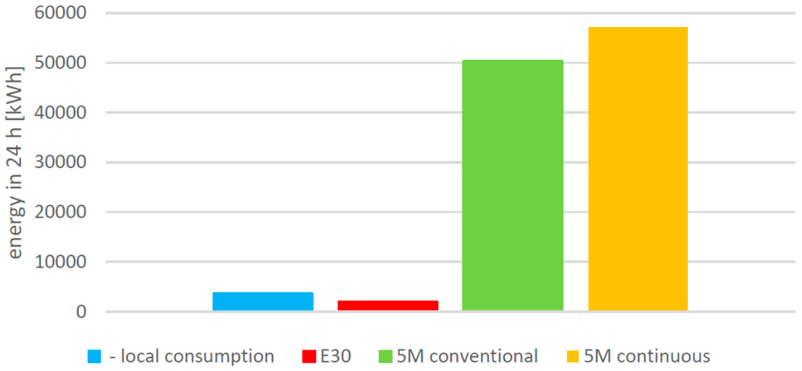
Since the primary purpose of wind power installations is the feed-in of electric energy, the energy yield is compared first. 
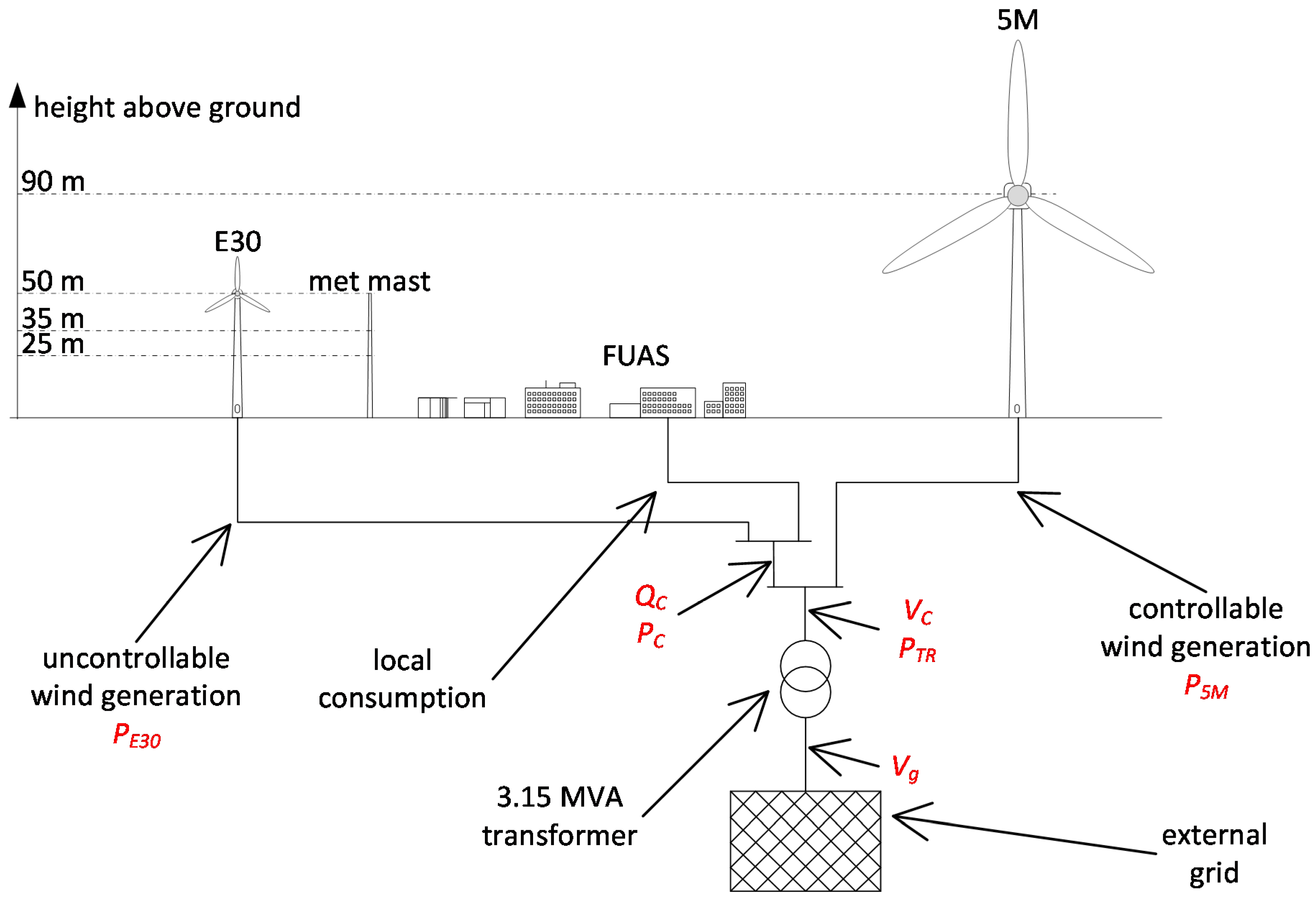
Figure 14 shows the energies that are fed into and consumed from the grid of campus Flensburg on 5 April 2017. The local consumption (3.67 MWh), which is partially provided by the E30 (1.97 MWh), is only a minor fraction of the energy produced by the 5M. Controlling the 5M with continuous feed-in management yields 57.1 MWh, which is 13.5% more than with conventional feed-in management.
It has to be pointed out however, that the numbers of MWh are not transferable to other cases as they apply only to the scenario considered here. These numbers do, however, allow the conclusion to be drawn that continuous feed-in management increases the energy yield substantially. The difference in energy yield would be even more striking were the voltage in the outer high voltage grid, Vg, assumed to be higher. In this case conventional feed-in management would lead to Pdem = 0.3 pu or even 0 pu most of the time. The same would apply when conventional feed-in management were to be conducted in the same precautionary manner, with the goal to minimise the control effort, as can be observed in reality [16]. Continuous feed-in management, on the other hand, responds to the instantaneous changes in the grid voltage and limits Pdem accordingly.
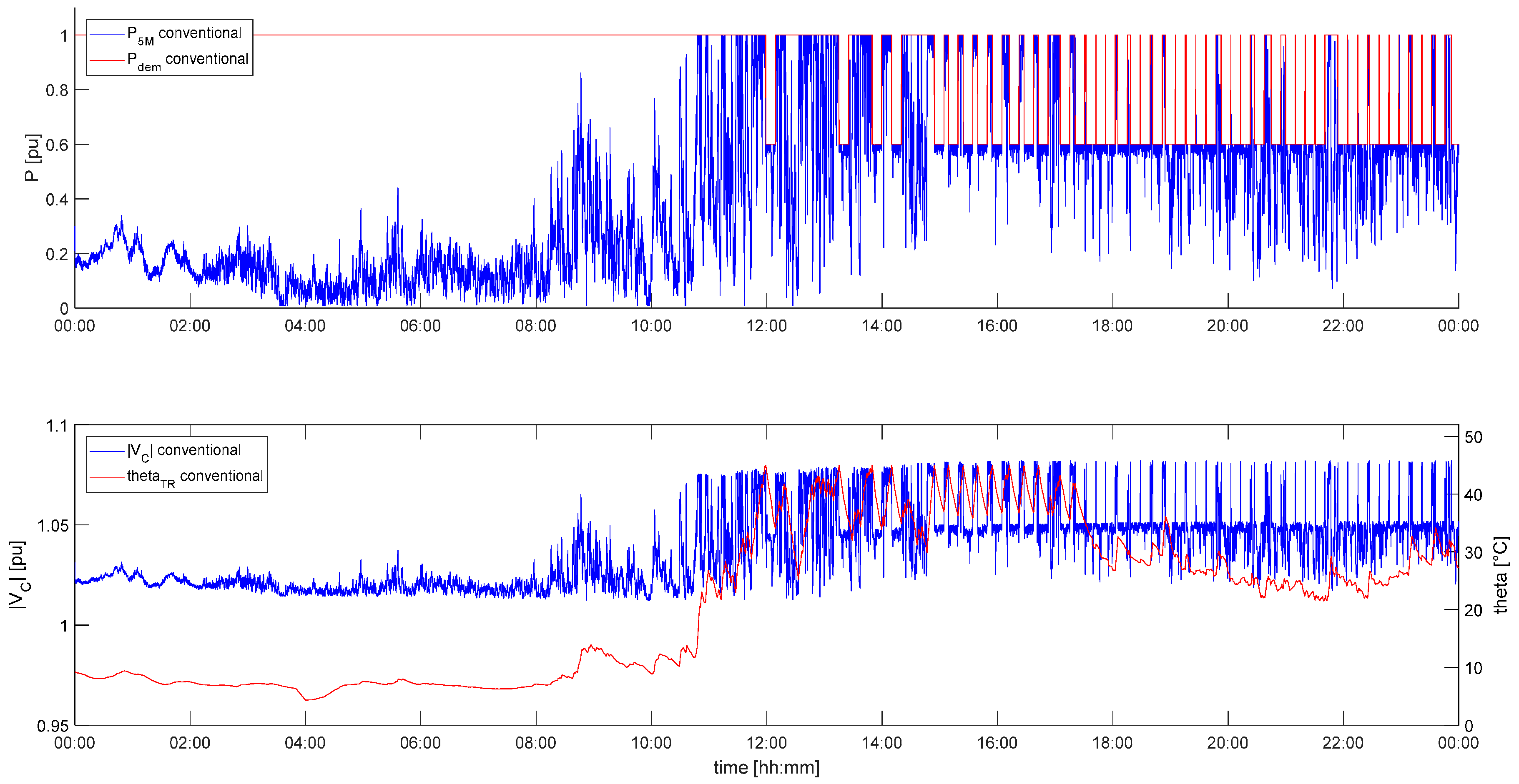
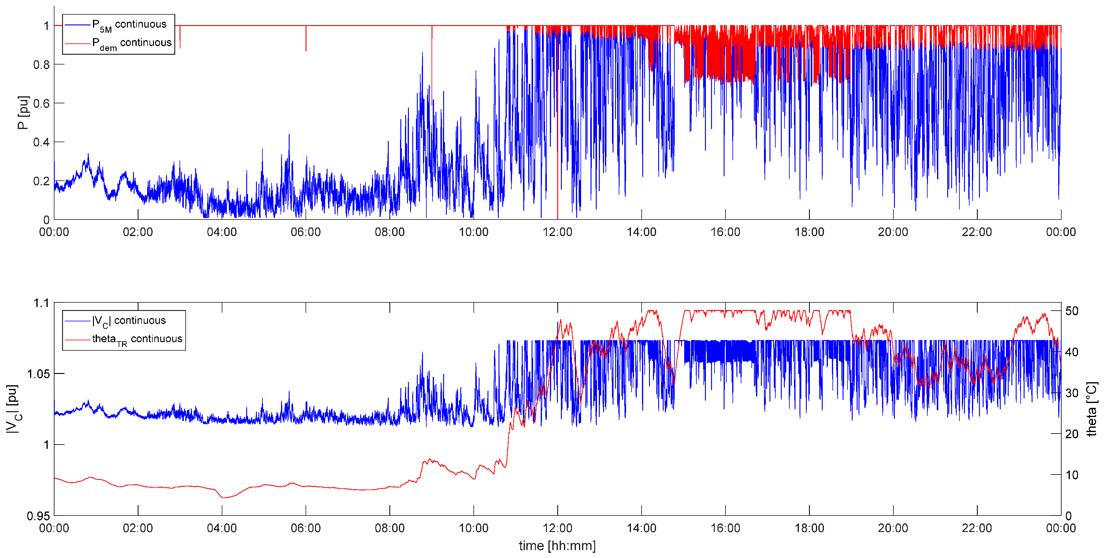
The thermal loading of the transformer is a measure for the utilisation of the same and of other assets in the power system. Comparing the transformer temperature after 12:00 (comparing Figure 12 and Figure 13) it can be seen that conventional feed-in management makes much more use of power system assets than conventional feed-in management. While continuous feed-in management keeps the transformer at its target temperature of 50 °C for several hours, in conventional feed-in management it barely reaches up to 45 °C.
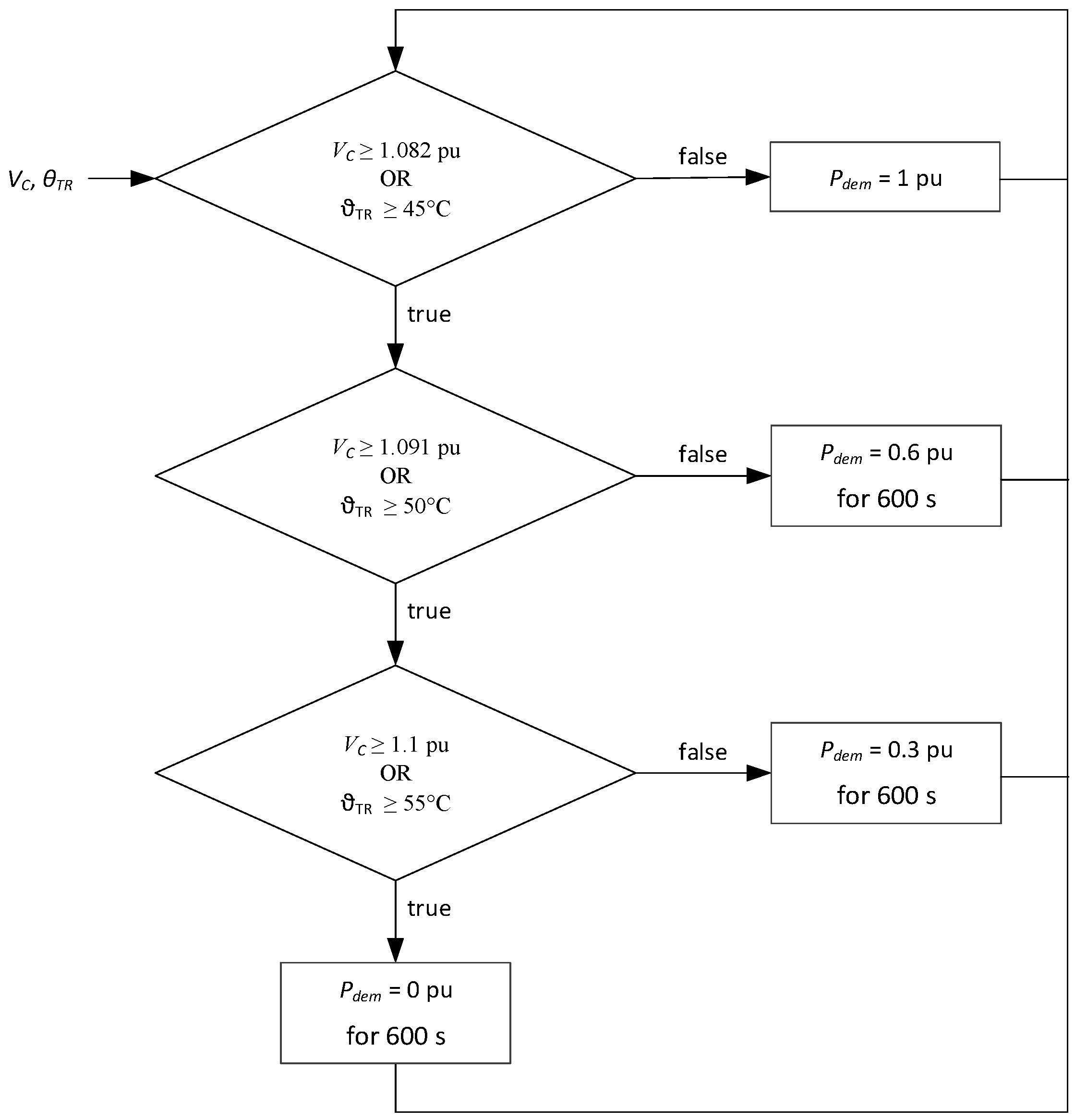
The variability of VC is a measure of the quality of the power fed into the power system. Over the whole day the lowest value of VC is 1.013 pu. In case of conventional feed-in management it regularly reaches up to 1.082 pu. In contrast to this, there is only one single peak where VC reaches up to 1.086 pu while it is controlled with continuous feed-in management. At all other times continuous feed-in management limits VC reliably to 1.073 pu.

4.2. Mechanical Loads in the WT

In power production operation a WT can experience excitation from four external sources: rotation, varying wind, varying terminal voltage, and varying Pdem. Controlling Pdem with respect to the loading of the power system to which the WT is connected, means decoupling the controls of the WT from the wind that instantaneously prevails at the rotor of the WT. This potentially means stress for the WT [8]. Such stress can be associated with two different categories:
  • Varying operating points and the necessity to level out variations by adjusting the pitch angle, potentially even with the maximum pitch rate.
  • Exciting resonances.
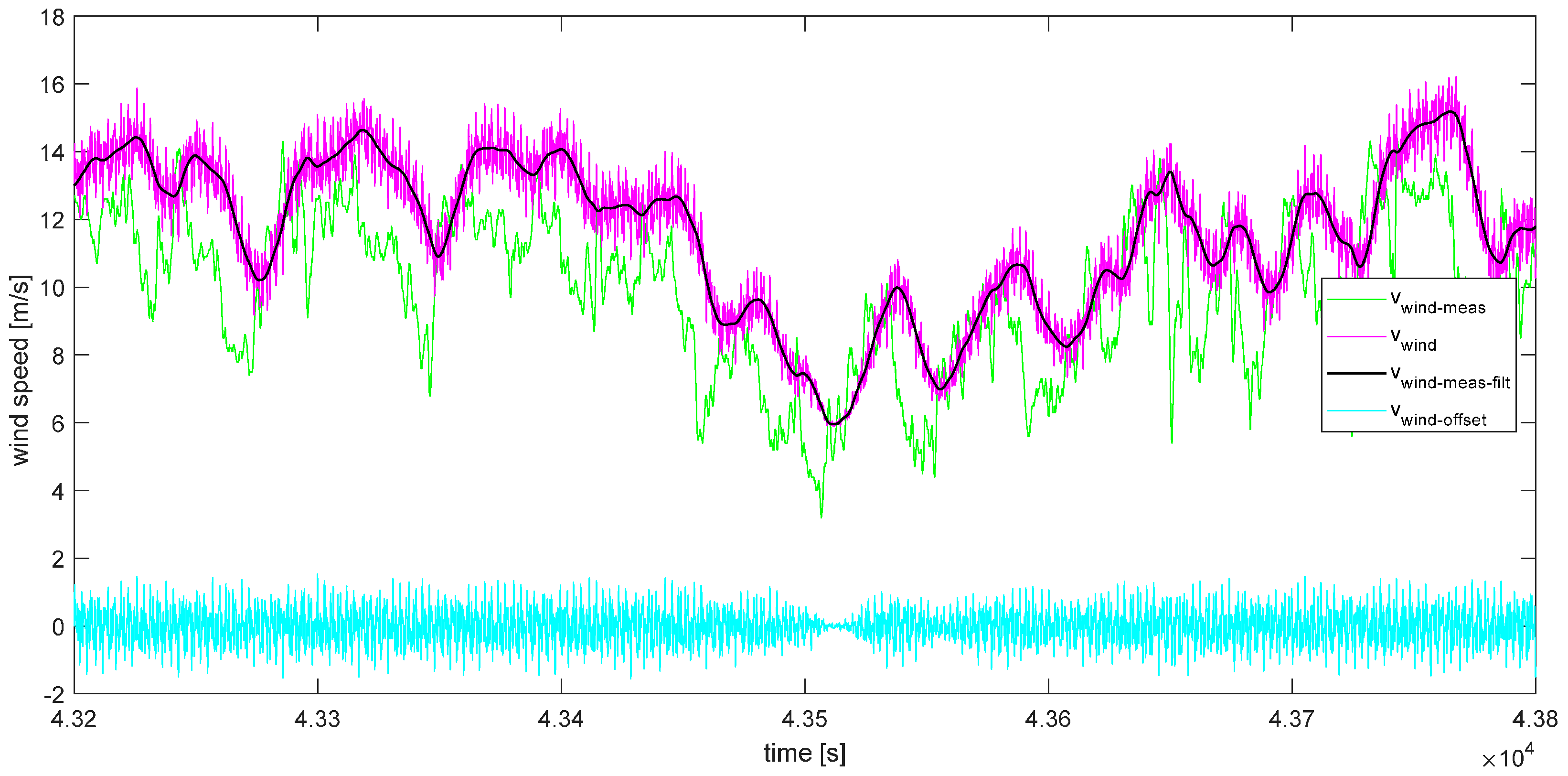
Vibrations are primarily excited by excitations that have the same frequency as the eigenfrequency of the vibrating WT component. Single excitation events, like a step change in a signal, are less harmful as they usually do not cause vibrations of constant or even increasing magnitude. It has to be noted that such single events might cause extreme loads that are not related to resonances, but such extreme events are not caused by feed-in management operation. Therefore, the persistent excitations to vibrations are assessed as follows. As discussed in 
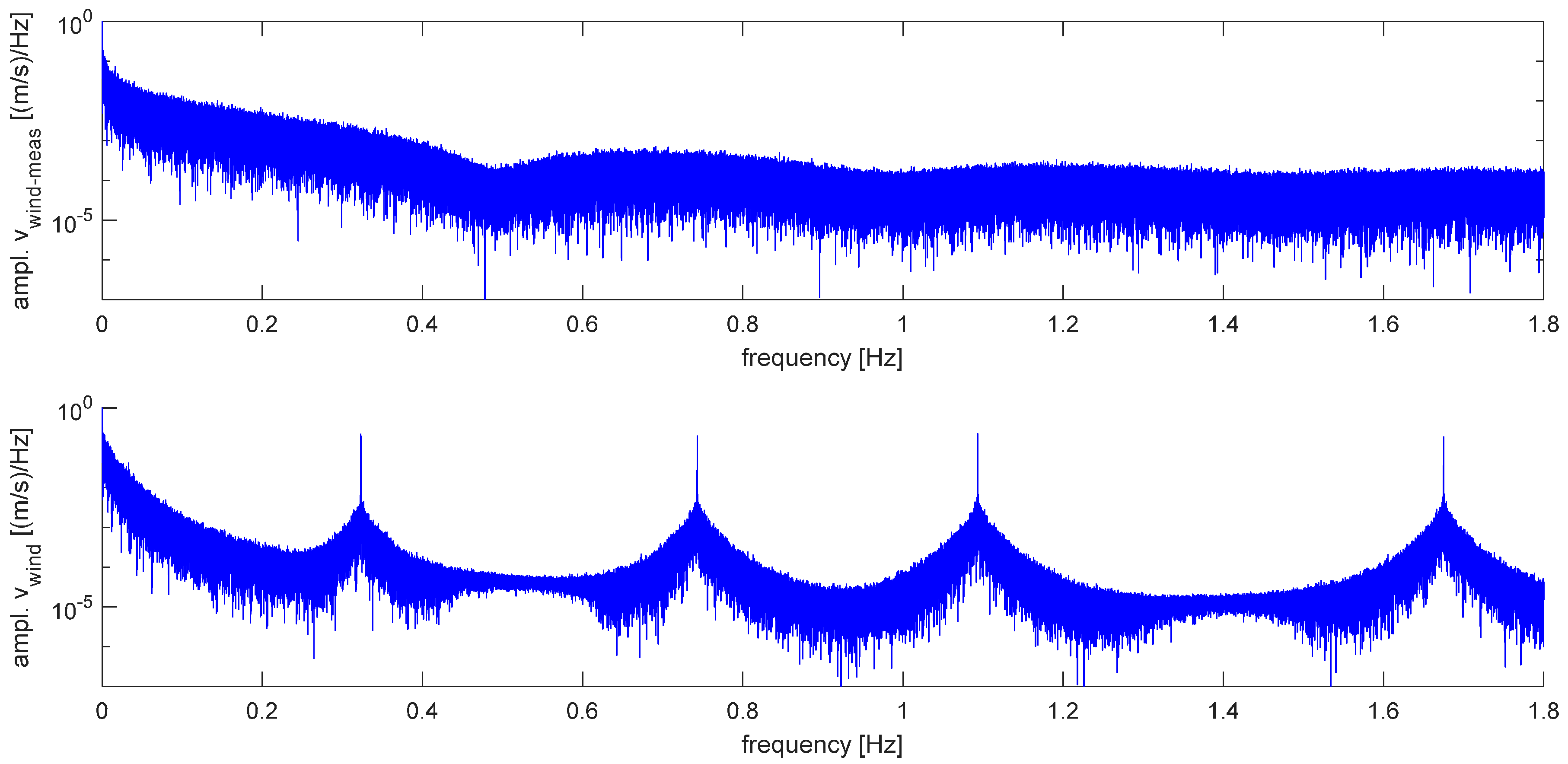
Section 2.6 “Wind Model”, the wind speed time series is offset with sinusoidal components that are of the same frequencies as the eigenfrequencies of the WT components. Hence, in addition to the stochastic natural wind speed variations, there are also wind speed variations that are directly targeted to excite the 5M to vibrations, see Figure 9. In the scenario simulated here the voltage (VC) has no significant effect, as it varies in a too narrow band. The other source of excitation is the 
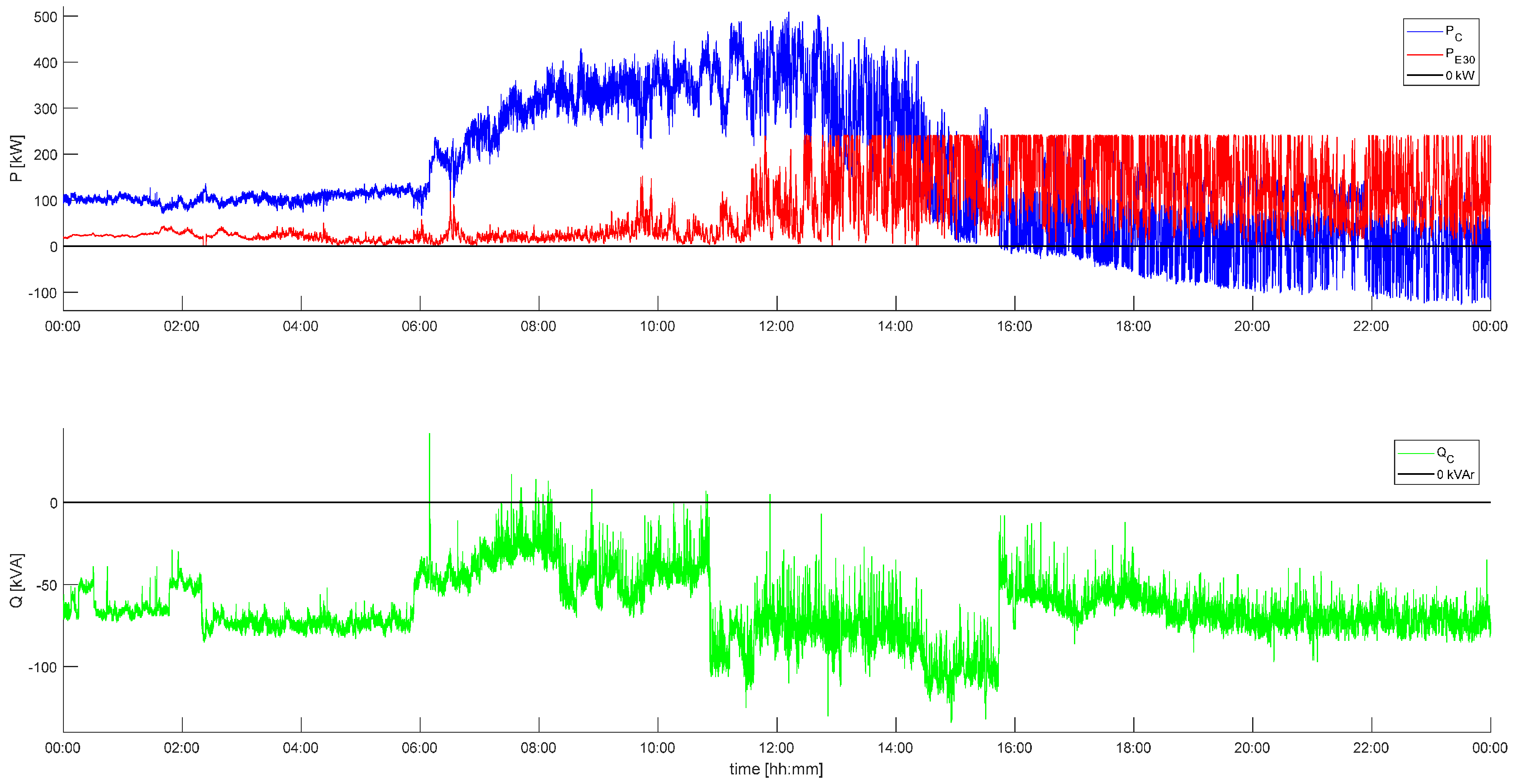
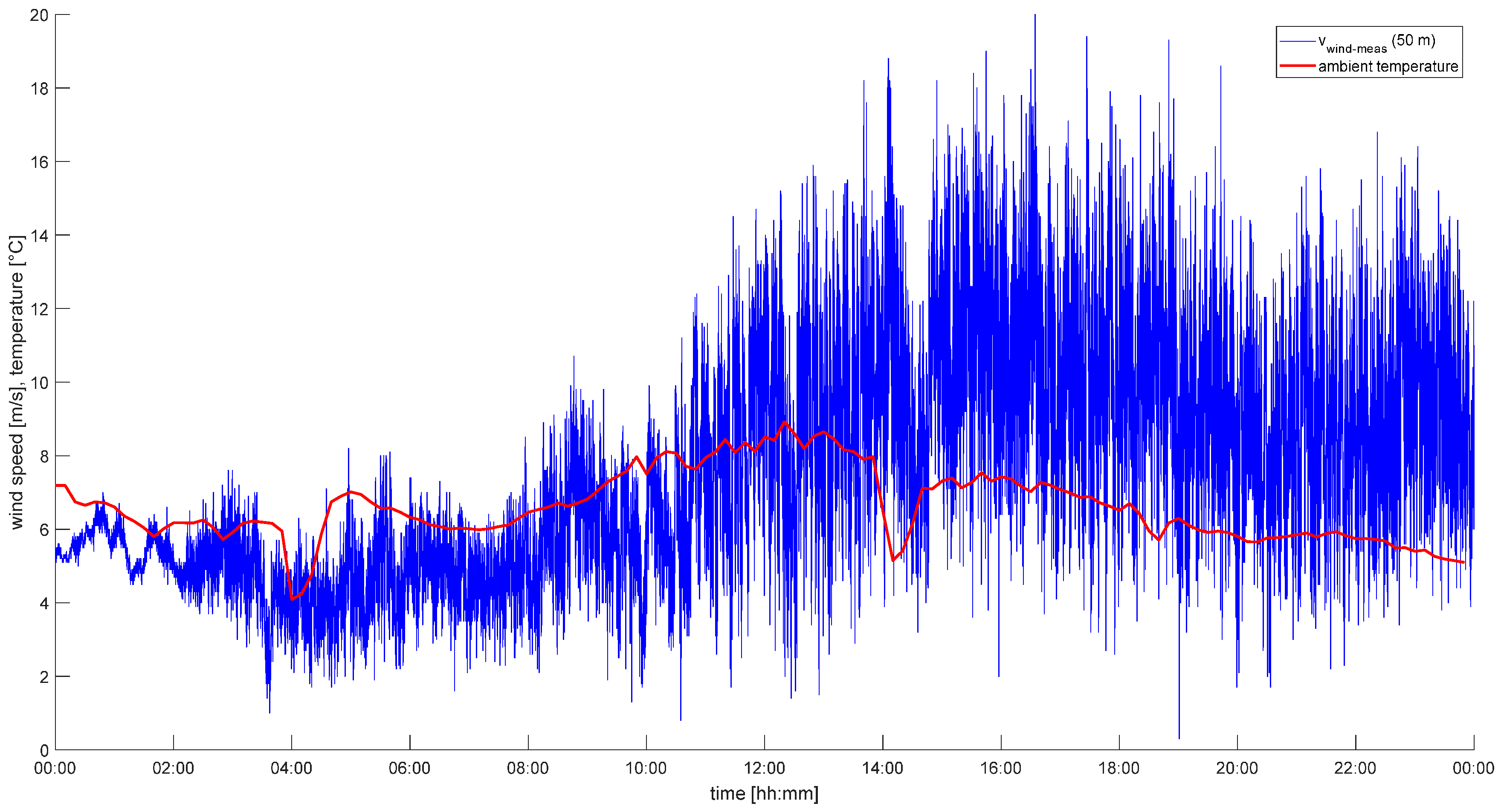
Pdem signal that results from the loading of the transformer. Hence, it is affected by the wind speed at the E30, vwind_meas, which leads to PE30, and together with the load power these add up to 
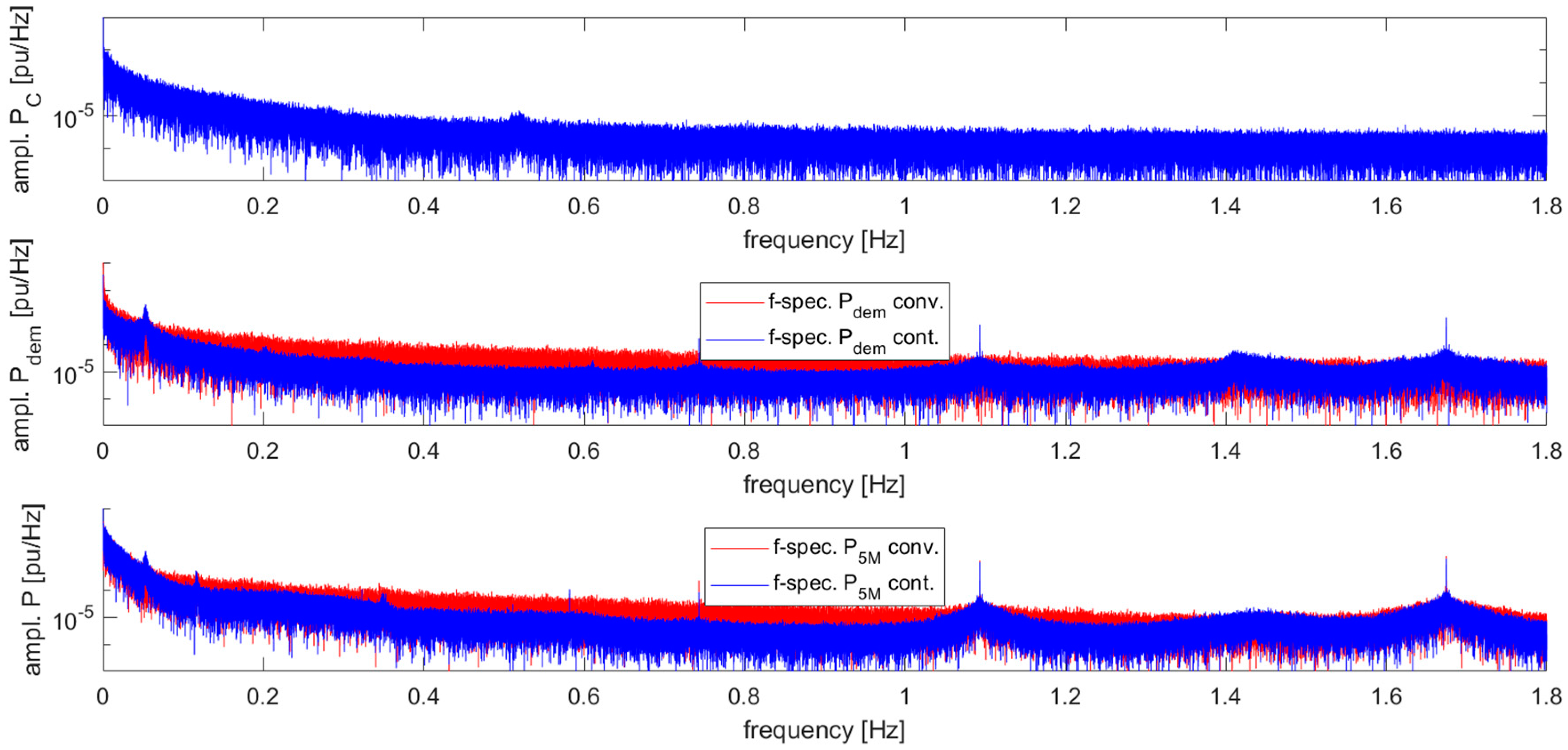
PC. In order to assess the potential to excite vibrations in the 5M, Figure 15 shows the frequency spectra of the different power signals. The frequency spectrum of PC comprises all relevant frequencies but does not exhibit any particular frequency peaks. The same applies to the Pdem signal of conventional feed-in management. The Pdem signal of continuous feed-in management comprises distinct frequencies that result from the heating up of the transformer and from the eigenfrequencies of the WT. Looking at Figure 10 it becomes obvious that the dynamics of both, the transformer, as well as the 5M, have a bearing on Pdem of continuous feed-in management. Consequently, these frequencies are reproduced in the power that the 5M feeds into the power system. In contrast to this, in conventional feed-in management the generator power of the 5M only exhibits the eigenfrequencies of the blades in the edgewise direction and the torsional eigenfrequency of the drive train. It barely exhibits the eigenfrequency of the blade in the flapwise direction and it does not exhibit the eigenfrequency of the tower of the 5M.
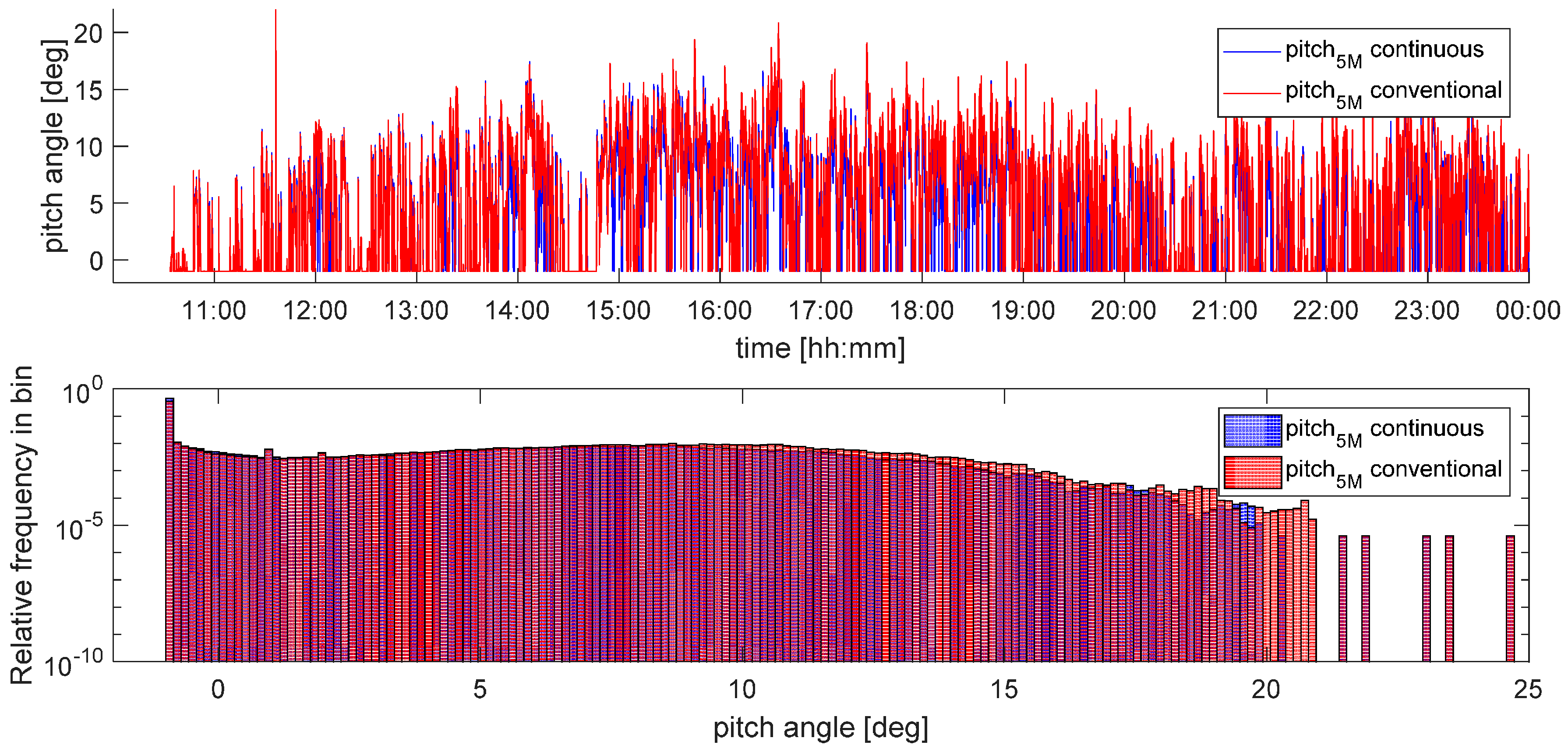
With these excitations the dynamic behaviour of the WT can be assessed. In the following figures, time traces are limited to the part of the day where feed-in management takes place. The units of the signals shown in some of the following graphs are per unit (pu), which relates to the rotational speed of the rotor. A detailed discussion of the units is omitted here, as this can be found in the documentation of the simulation model [10]. The following figures also show the distribution of the frequencies with which the different values occur in the time traces. (Blue bars are for continuous feed-in management, red bars are for conventional feed-in management and dark red areas show overlap of blue and red bars.)
Figure 16 shows that the pitch angle of the 5M varies in the same range in both cases. There are differences in the frequency distribution for pitch angles above 10 deg, which should not be overrated due to the logarithmic scale.
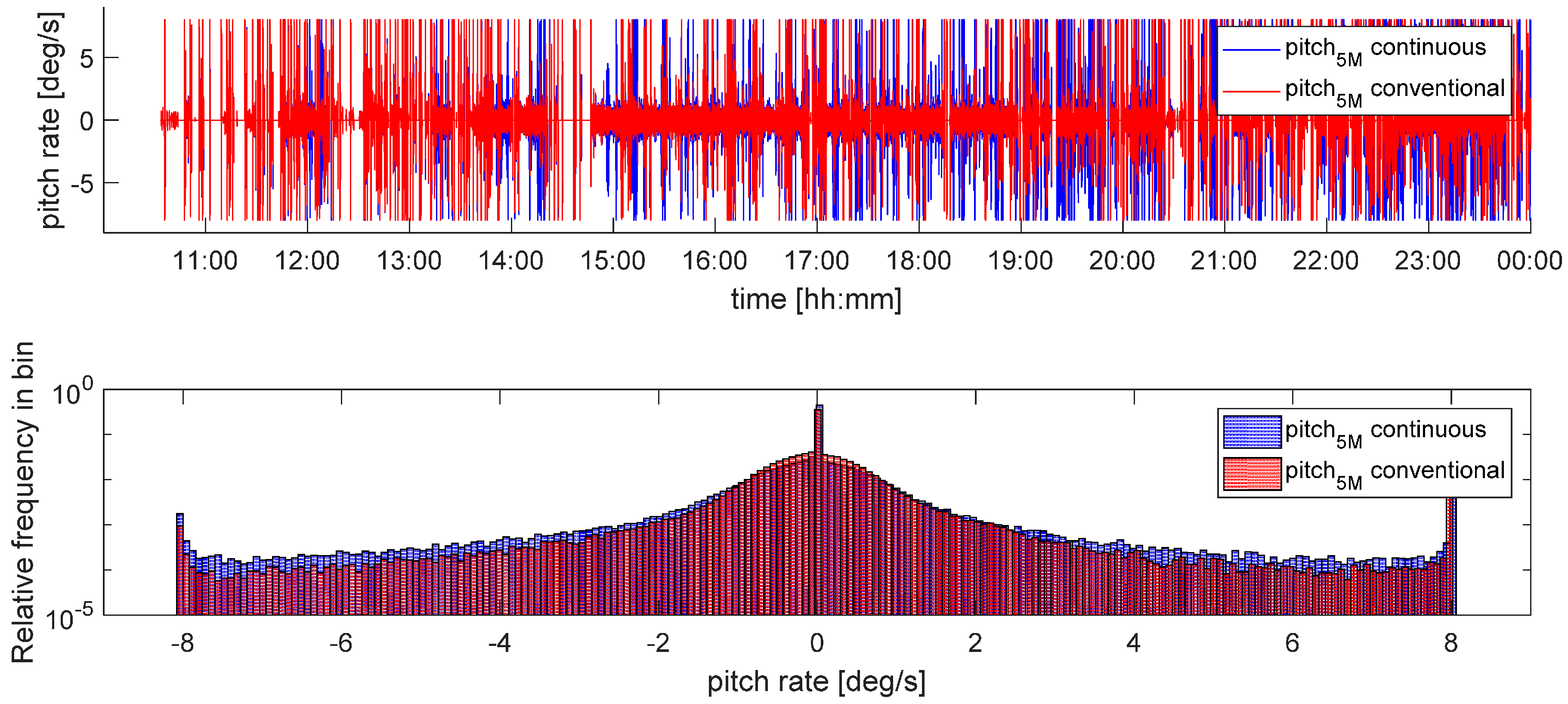
The pitch rates are also comparable, as can be seen in Figure 17. In both cases they regularly reach −8 deg/s and 8 deg/s, which is the maximum pitch rate of the 5M. Continuous feed-in management causes only somewhat more frequent high pitch rates. (Again, when looking at Figure 17 it has to be kept in mind that the relative frequency of the pitch rates is plotted on a logarithmic scale.) This might appear surprising at first sight, as it could be suspected that maintaining a constant Pdem (conventional feed-in management) requires less pitching actions than continuously varying Pdem (continuous feed-in management). Comparing Figure 12 and Figure 17 reveals that conventional feed-in management, on average, requires somewhat lower pitch rates. However, a constant Pdem still requires drastic pitching actions, as the wind speed still varies. This effect becomes more dominant for higher wind speeds or lower Pdem as these two variables have an effect on the pitch sensitivity [8].
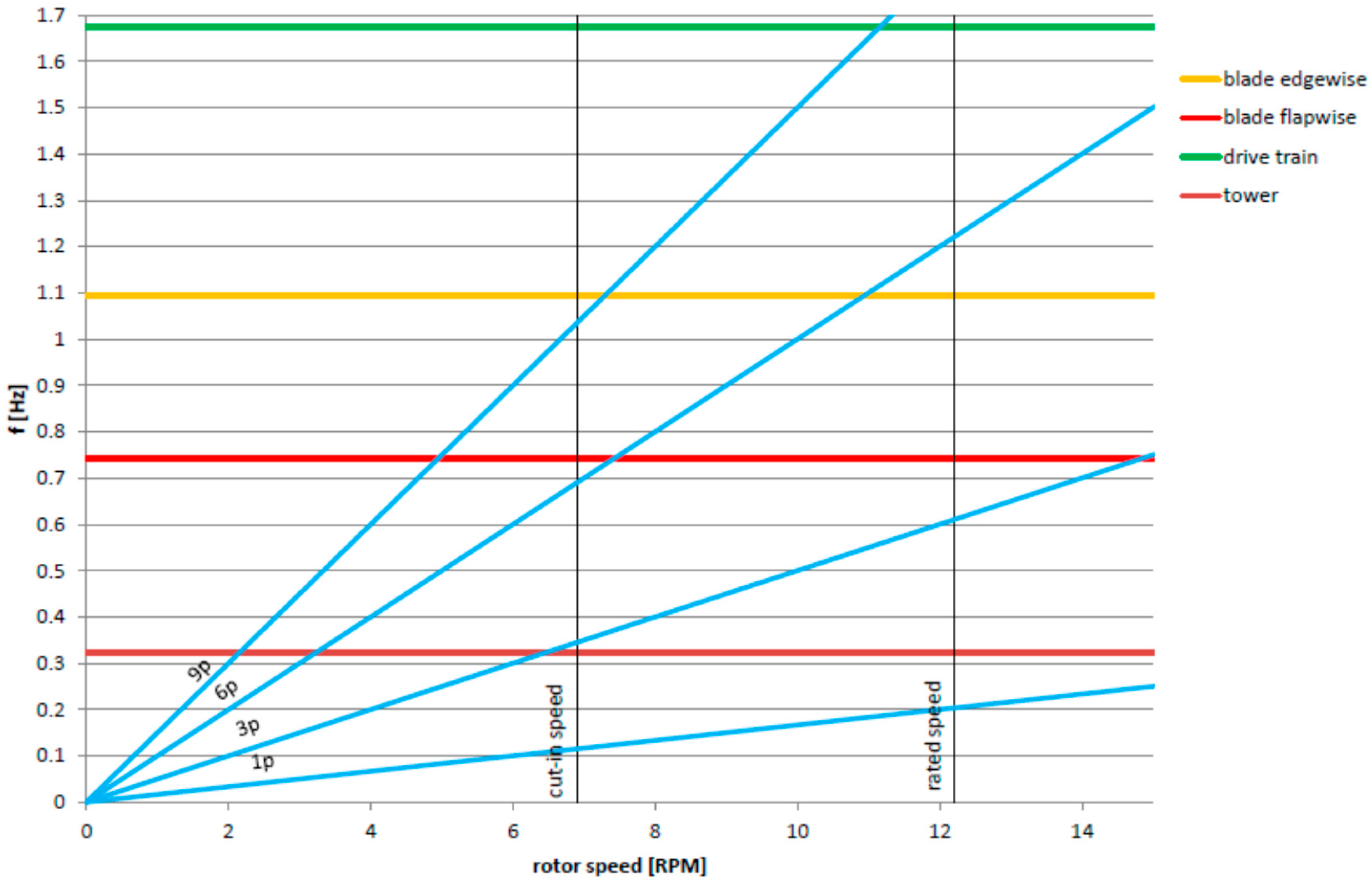
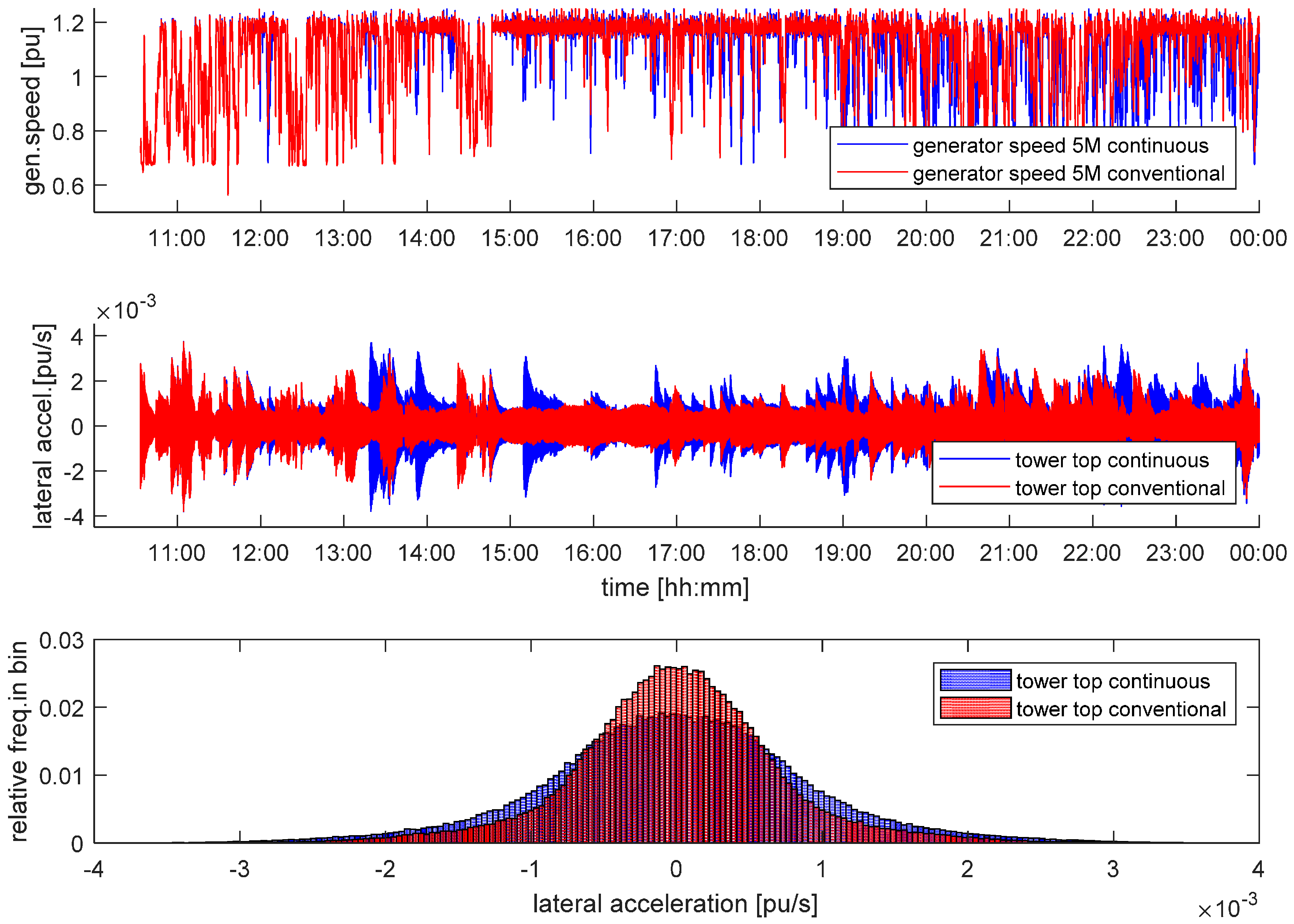
Another measure for mechanical stress is the acceleration of the tower top, which can occur in the lateral direction (in rotor plane direction) and in the longitudinal direction (in out of rotor plane direction). Excitation in the lateral direction is mainly caused by imbalances in the rotor. To emulate imperfections in manufacturing one of the rotor blades of the 5M is 100 kg heavier than the other two. This imbalance in the rotor leads to lateral excitation, especially when the rotor speed is close to the eigenfrequency of the tower. Looking at Figure 3 makes it obvious that whenever the rotational speed of the rotor is low, the 3p excitation is close to the eigenfrequency of the tower. To illustrate cause and effect of this phenomenon Figure 18 shows the rotational speed, the resulting lateral acceleration of the tower, and the frequency distribution of this acceleration.
Figure 18 reveals that the lateral vibrations of the tower top occur more often in case of continuous feed-in management. This is obvious as in continuous feed-in management the power varies on a regular basis, leading to more variations of the rotor speed.
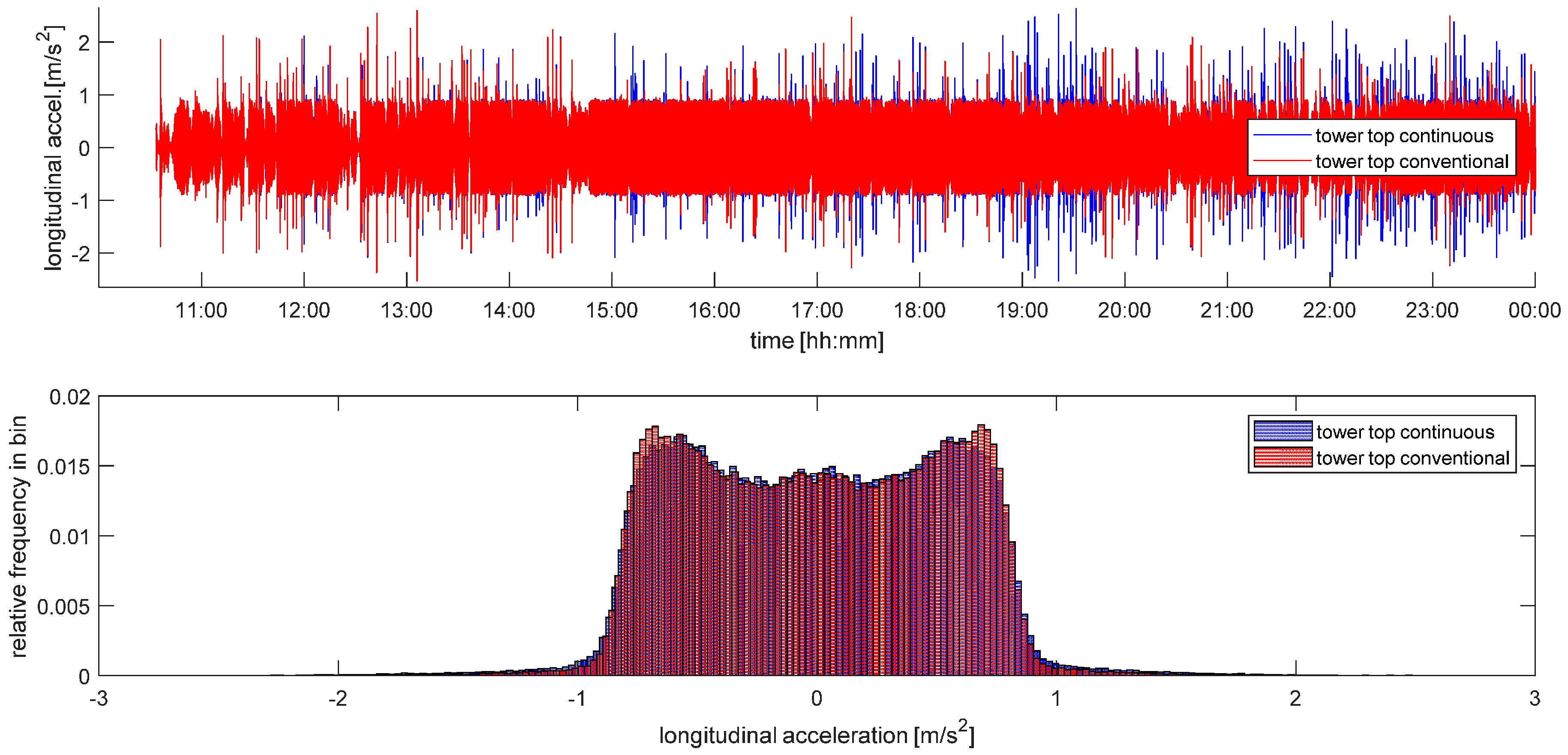
Tower vibrations in the longitudinal direction are mainly caused by wind speed variations and pitch angle variations. In particular pitch angle variations with high pitch rates have drastic effects on the thrust of the rotor, and hence, excite the tower in the longitudinal direction. While the time traces of the wind speed are comparable for both scenarios, the pitch variations are considerably different, as can be seen in Figure 16 and Figure 17.
Figure 19 shows the tower top acceleration of the 5M in the longitudinal direction. It can be seen that the tower is more strongly excited when Pdem requires pitch angle variations with high pitch rates. Consequently, continuous feed-in management causes somewhat more frequent higher accelerations in the longitudinal direction.
In the longitudinal direction a persistent vibration with the eigenfrequency of the tower, ft, and with a magnitude of about 0.9 m/s² is observable almost all the time. There is a constant excitation in the wind, because ft is contained in the wind speed signal (compare Figure 9). In the lateral acceleration such persistent vibrations are not contained, because the drive train speed, which is the primary cause for lateral tower vibrations, varies all the time. Therefore, excitation in the lateral direction from the imbalance in the rotor happens at different frequencies.
Looking at Figure 18 and Figure 19 it can be seen that conventional feed-in management causes fewer single excitations of the tower. However, the maximum accelerations (height of the peaks in Figure 18 and Figure 19) are identical in both types of feed-in management. The persistent vibrations in the longitudinal direction are also identical. Figure 18 further shows that the variation of the generator speed does not exhibit persistent or even unstable vibrations.
The remaining degrees of freedom of the WT model are the motions of the blade tip with respect to the blade root in the in-plane direction and in the out-of-plane direction. 
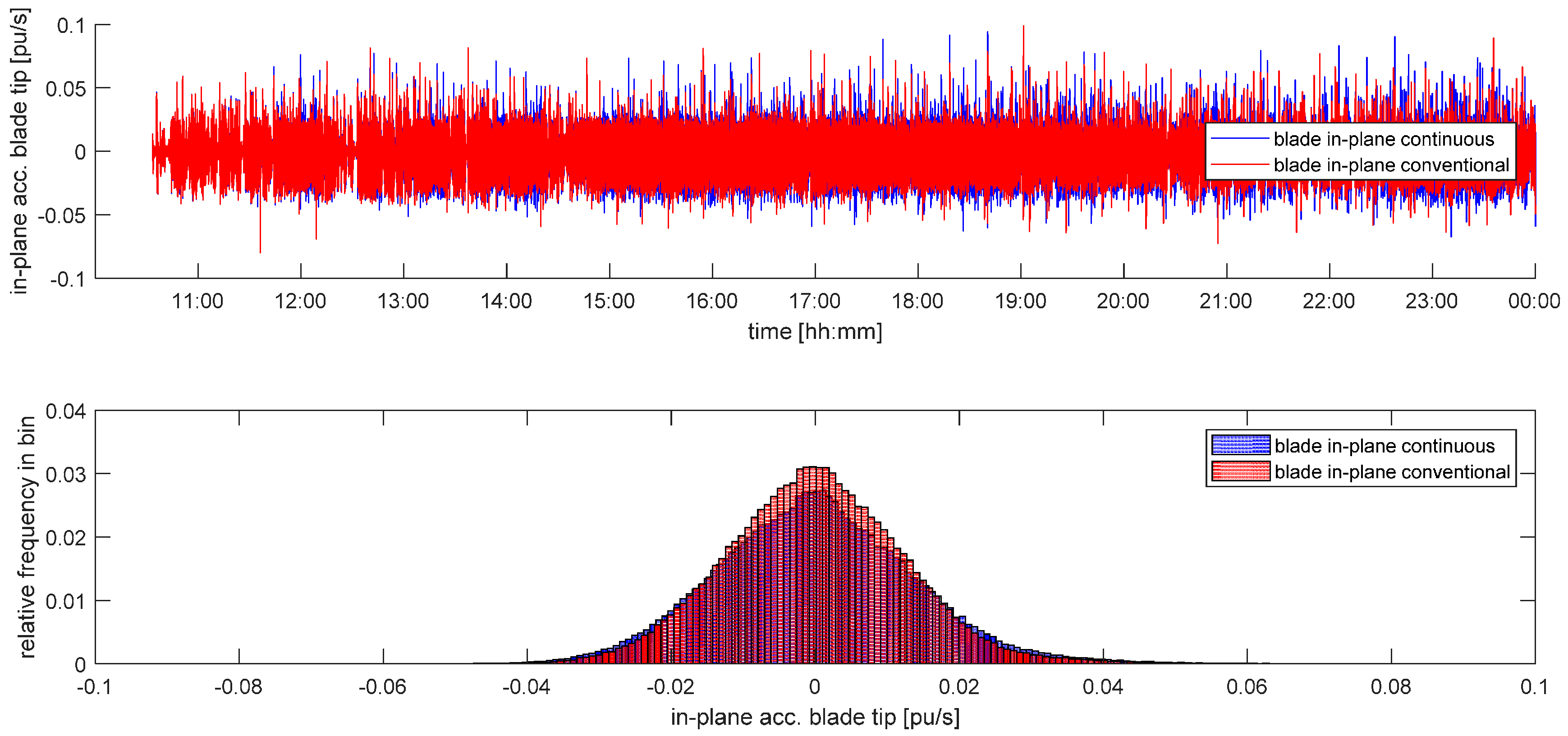
Figure 20 shows the accelerations that the blade tip section of one arbitrary blade of the 5M experiences in the in-plane direction. The acceleration in the in-plane direction exhibits a persistent vibration with a magnitude of about 0.03 pu/s most of time. This acceleration is mainly caused by the rotation of the rotor, i.e., alternating gravitational forces that act on the rotor blade. In addition, also the wind speed variations, which have the same frequency as the blade eigenfrequency in the in-plane direction cause such vibrations. The diagram in Figure 7 reveals that the magnitude of this wind speed component is constantly high when the wind speed is high. Beyond this persistent vibration, variations in in-plane acceleration are caused by varying operating points. Therefore, continuous feed-in management causes somewhat more frequent higher in-plane acceleration than conventional feed-in management. The only rarely occurring high peaks that arise from drastic changes in instantaneous wind speed at the blade, or from drastic changes in operating point are comparable in both scenarios.
Figure 21 shows that the acceleration in the out-of-plane direction exhibits a persistent vibration with a magnitude of about 5 m/s² most of the time. This acceleration is mainly caused by the variations in thrust forces that result from wind shear and rotation of the rotor. Wind speed variations that are of the same frequency as the out-of-plane blade eigenfrequency also directly cause acceleration out-of-plane. Beyond this persistent vibration, variations in out-of-plane acceleration are to a minor extent caused by varying operating points. Therefore, continuous feed-in management causes somewhat more frequently occurring out-of-plane accelerations of moderate magnitude.
The persistent vibrations are either caused naturally by the rotation of the rotor, or by the deliberately added sinusoidal wind speed components. The sole purpose of these wind speed components is to excite the eigenfrequencies of the WT. Despite these persistent excitations, there are no vibrations with large magnitude that persist for long, or whose magnitude even increases because they are excited by continuous feed-in management. The stochastic nature of the excitations ensure that the WT never dwells long enough in one operating point so that an eigenmode develops vibrations with a critical magnitude [8]. Even if such critical excitation persists, the aerodynamic damping helps to avoid the vibrations becoming unstable.

5. Conclusions

It is a common problem that wind power installations grow faster than the power system, into which these installations feed their power. In order to avoid thermal overloading of the power system and unfavourable voltages, it is common practice for power system operators to restrict the power that WTs may feed into the affected system: known as feed-in management. Currently, it is state of the art that feed-in management is optimised to serve the compromise between control effort and lost electric energy yield. Therefore, the direct connection between the current loading of the power system and the maximum power that WTs are allowed to feed in is lost completely. Consequently, the power system assets are not utilised to their full potential and large amounts of wind energy are wasted.
To avoid these problems continuous feed-in management is assessed in this paper. The idea is that the value, to which WT power is limited, is adjusted continuously. Hence, at any time WTs feed in just as much power as is acceptable for the power system. This leads to the maximum wind energy yield and the maximum utilisation of power system equipment.
The continuous feed-in management applied in this paper is assessed by means of a realistic case study. In this case study the WT that causes the overloading of the power system is first controlled with conventional feed-in management. The result of this simulation is used as reference in order to have a benchmark for assessing the performance of continuous feed-in management, which is simulated in the second step.
From a power system’s point of view, continuous feed-in management proves to be superior, both in terms of voltage and in terms of utilisation of the thermal capacity of the considered power system transformer. In addition, the wind energy yield is much larger. In the case considered here continuous feed-in management leads to a wind energy yield that is 13.5% larger compared to conventional feed-in management. It has to be mentioned that the conventional feed-in management simulated here is done without any precautionary reductions of the power limit as can be observed in reality. Otherwise the difference in energy yield would be even larger.
From a WT’s point of view a continuously varying power demand value causes more frequent and more rapidly changing operating points. A measure for this is the variation in the pitch angle and the frequency of occurrence of high pitch rates. However, this increased stress on the WT is not as large as expected, because a constantly reduced power demand (conventional feed-in management) also leads to stress due to the wind speed variations and the operating point dependent pitch sensitivity.
Looking at all degrees of freedom that are represented in the WT model used in this study, allows the mechanical stress to be assessed in terms of accelerations. It can be seen that continuous feed-in management causes somewhat more frequent accelerations. Hence, the fatigue loads are expected to be higher than in the case of conventional feed-in management. The peaks in the acceleration, however, are not larger compared to the peaks resulting from conventional feed-in management. Hence, it can be concluded that continuous feed-in management is an appropriate method for increasing wind energy yield without the need for massive over-dimensioning of the affected power system components.

Acknowledgments

This paper presents some results of the research project Untersuchung des dynamischen Verhaltens getriebeloser WEA im Hinblick auf Leistungsbereitstellung im Netz im Minuten und Sekundenbereich. This work was carried out by the Wind Energy Technology Institute at Flensburg University of Applied Sciences in co-operation with DNV GL GmbH. The authors acknowledge the financial support to the project by the Gesellschaft für Energie und Klimaschutz Schleswig-Holstein GmbH (EKSH) project number 8/12-6. The authors further acknowledge the support in conducting the measurements on Campus Flensburg by Thomas Haase and Dirk Albert.

Author Contributions

Clemens Jauch conceived the concepts presented in this paper. He created the simulation model, conducted the simulations and wrote the paper. Arne Gloe set up the power measurement system at the grid connection point of campus Flensburg. He further contributed to the technical discussions and reviewed the paper. Henning Thiesen contributed to the data acquisition and designed the interface between measurements and simulations. He further contributed to the technical discussions and reviewed the paper. Sebastian Hippel yielded the parameters of the 5M, contributed to the technical discussions and reviewed the paper.

Conflicts of Interest

The authors declare no conflict of interest. The founding sponsors had no role in the design of the study; in the collection, analyses, or interpretation of data; in the writing of the manuscript, and in the decision to publish the results.

Appendix A

Table A1. Parameters of grid connection transformer.
NameValueUnitDescription
Vrated24,000Vrated voltage
uk6%short circuit voltage
Srated3150,000VArated apparent power
Pscl27500Wshort circuit power
frated50Hzrated frequency
mTR6100kgtotal mass of transformer
moil1070kgmass of oil in transformer
mAl1100kgmass of aluminium conductor
Acool111m²cooling surface of transformer
cTR786Ws/kg/Kspecific heat capacity of transformer
αTR100W/m²/Kheat transfer coefficient of cooling air
Table A2. Parameters of WT model.
NameValueUnitDescription
fbf0.7429Hz1st eigenfrequency blade bending flapwise
fbe1.0931Hz1st eigenfrequency blade bending edgewise
ft0.3230Hz1st eigenfrequency tower bending
fdt1.6749Hz1st eigenfrequency drive train torsion
Table A3. Lookup table A(vwind_meas_filt) in wind model.
Wind Speed (90 m) [m/s]Magnitude [m/s]
3.190.07
4.580.02
5.870.02
7.650.25
9.790.35
12.240.40
15.370.40
Table A4. Parameters of temperature controller and Pdem controller.
Temperature ControllerValueUnit
Proportional gain 0.1pu/°C
Integral gain0.9pu/°C/s
Pdem ControllerValueUnit
Proportional gain 3pu/pu
Integral gain9pu/pu/s
VC [pu]Pmax_TR_volt [pu]
01
1.071
1.10

References

  1. Federal Ministry for Economic Affairs and Energy, Germany. Act on the Development of Renewable Energy Sources. Available online: http://www.bmwi.de/Redaktion/EN/Downloads/renewable-energy-sources-act-eeg-2014.html (accessed on 22 June 2017).
  2. Tenne, T.; Holding, B.V. Operation and Usage—How does Feed-in Management Work? Available online: https://www.tennet.eu/electricity-market/german-market/eeg-kwkg/feed-in-management/operation-and-usage/ (accessed on 22 June 2017).
  3. Monitoring Report 2015. Available online: https://www.bundesnetzagentur.de/SharedDocs/Downloads/EN/BNetzA/PressSection/ReportsPublications/2015/Monitoring_Report_2015_Korr.pdf?__blob=publicationFile&v=4 (accessed on 5 May 2017).
  4. Monitoring Report 2016. Available online: https://www.bundesnetzagentur.de/SharedDocs/Downloads/DE/Sachgebiete/Energie/Unternehmen_Institutionen/DatenaustauschUndMonitoring/Monitoring/Monitoring2016/MonitoringSummary2016.pdf?__blob=publicationFile&v=2 (accessed on 22 June 2017).
  5. Jauch, C. FH Flensburg Erforscht Dynamische Leistungsbereitstellung Durch WEA; Ingenieurspiegel: Bingen, Germany, 2013; pp. 20–21. (In German) [Google Scholar]
  6. Wieben, E. Der 5%-Ansatz im Kontext der Netzqualität. In Proceedings of the Energiesymposium Westküste, Heide, Germany, 10 September 2015. (In German). [Google Scholar]
  7. FGW, RWTH Aachen. Abschlusspräsentation zur Systemstudie zum Einspeisemanagement Erneuerbarer Energien; Oldenburg, Germany, 9 July 2015. Available online: http://de.slideshare.net/EWE_AG/20150702-abschlussprsentation-systemstudie-einspeisemanagementfinal (accessed on 22 June 2017). (In German).
  8. Jauch, C.; Gloe, A. Improved feed-in management with wind turbines. In Proceedings of the 15th Wind Integration Workshop, Vienna, Austria, 15–17 November 2016. [Google Scholar]
  9. Jonkman, J.; Butterfield, S.; Musial, W.; Scott, G. Definition of a 5-MW Reference Wind Turbine for Offshore System Development. Available online: http://pop.h-cdn.co/assets/cm/15/06/54d150362c903_-_38060.pdf (accessed on 22 June 2017).
  10. Jauch, C. First Eigenmode Simulation Model of a Wind Turbine—For Control Algorithm Design, 21 December 2016; WETI Hochschule: Flensburg, Germany, 2016. [Google Scholar]
  11. Gloe, A.; Jauch, C. Simulation Model Design and Validation of a Gearless Wind Turbine 23 March 2016; WETI Fachhochschule: Flensburg, Germany, 2016. [Google Scholar]
  12. Jonkman, J.; Jonkman, B. Fast modularization framework for wind turbine simulation: Full-system linearization. In Proceedings of the Science of Making Torque from Wind (TORQUE 2016), Munich, Germany, 5–7 October 2016. [Google Scholar]
  13. Schaffarczyk, A. Understanding Wind Power Technology, Theory, Deployment and Optimisation; Wiley: New York, NY, USA, 2014. [Google Scholar]
  14. Standard Transformatoren ismet GmbH, VS-Schwenningen, Germany. Available online: http://www.ismet.de/de/downloads (accessed on 22 June 2017). (In English).
  15. Fischer, R. Elektrischer Maschinen, 10th ed.; Carl Hanser Verlag: München, Germany, 2000. (In German) [Google Scholar]
  16. Regionen mit Einspeisemanagement—Abgeschlossene Einsätze des Einspeisemanagement—SH Netz Mittel-und Hochspannung, TenneT Höchstspannung, 2017. Available online: https://www.sh-netz.com/cps/rde/xchg/sh-netz/hs.xsl/3972.htm (accessed on 22 June 2017). (In German).
Figure 1. Setup of case study of campus Flensburg supplemented by a 5 MW wind turbine (WT) with connection to the external grid.
Energies 10 00870 g001
Figure 2. Power measurements on campus Flensburg on 5 April 2017.
Energies 10 00870 g002
Figure 3. Campbell diagram with eigenfrequencies of 5M WT as implemented in the 1st eigenmode model.
Energies 10 00870 g003
Figure 4. Wind speed at 50 m above ground (hub height of the E30) and temperature on campus measured on 5 April 2017.
Energies 10 00870 g004
Figure 5. Measured and extrapolated wind speed (a) and turbulence intensity, TI; (b) versus height above ground, z2.
Energies 10 00870 g005
Figure 6. Computed from measurements and extrapolated turbulence intensity, TI, versus wind speed.
Energies 10 00870 g006
Figure 7. (a) Block diagram of wind model; (b) content of lookup table A = f(vwind_meas_filt).
Energies 10 00870 g007
Figure 8. Measured wind speed at 50 m, filtered, extrapolated and offset wind speed at 90 m in the 10 Min interval at midday on 5 April 2017.
Energies 10 00870 g008
Figure 9. Frequency spectrum of wind speed measured at 50 m (top) and of the wind speed signal input to the 5M (bottom).
Energies 10 00870 g009
Figure 10. Power control circuit that maximises the power infeed while maintaining a healthy transformer temperature and an acceptable voltage in the campus grid.
Energies 10 00870 g010
Figure 11. Flow chart of conventional feed-in management.
Energies 10 00870 g011
Figure 12. Simulation of case study with conventional feed-in management.
Energies 10 00870 g012
Figure 13. Simulation of case study with continuous feed-in management.
Energies 10 00870 g013
Figure 14. Comparison of energies fed into and consumed from the campus grid during the 24 h scenario.
Energies 10 00870 g014
Figure 15. Frequency spectra of power. Top: of PC; middle: of power setpoint, Pdem, from feed-in management; bottom: of P5M.
Energies 10 00870 g015
Figure 16. Pitch angle (top) and frequency distribution of pitch angles (bottom) of 5M.
Energies 10 00870 g016
Figure 17. Pitch rate (top) and frequency distribution of pitch rate (bottom) of 5M.
Energies 10 00870 g017
Figure 18. Rotational speed of drive train (top), lateral acceleration of tower top of the 5M (middle) and frequency distribution of lateral acceleration (bottom).
Energies 10 00870 g018
Figure 19. Longitudinal tower top acceleration of the 5M (top) and frequency distribution of this acceleration (bottom).
Energies 10 00870 g019
Figure 20. In-plane acceleration of blade tip section with respect to blade root section of one arbitrary blade of the 5M (top) and frequency distribution of this acceleration (bottom).
Energies 10 00870 g020
Figure 21. Out-of-plane acceleration of blade tip section with respect to the blade root section of one arbitrary blade of the 5M (top) and frequency distribution of this acceleration (bottom).
Energies 10 00870 g021

