This subsection is devoted to describing the basic mathematical modeling of the examined system. The presented equations concern energy balances, index definitions and other useful modeling assumptions.
2.3.1. Solar Field Modeling
In
Section 2.3.1, a detailed thermal modeling for the Eurotrough module is presented. These equations can be combined together and finally, the thermal efficiency of the solar collector can be calculated in every case. Parabolic trough collectors are imaging concentrating collectors with high concentration ratio and they exploit only the direct beam part of the incident solar irradiation [
36]. Thus, the available solar energy is calculated as the product of the outer aperture (
Aa) and the solar direct beam irradiation (
Gb):
The outer absorber area is calculated according to Equation (6), using the outer absorber diameter (
Dro) and the length (
L) of the evacuated tube. The inner absorber area, as well as the cover areas (inner and outer), can be calculated with similar formulas as Equation (6):
The useful energy that the heat transfer fluid gains are able to be calculated according to the energy balance of its volume, as it is given in Equation (7). It is important to state that this quantity represents the useful heat of one module of the total system. The specific heat capacity (
cp) corresponds to the working fluid of the solar collector which is nanofluid in the majority of the cases and pure thermal oil in only some cases:
It is useful to state that the mass flow rate (
m) is calculated as the product of the fluid density (
ρ) and the volumetric flow rate (
V):
The most important index for the evaluation of the solar collector is the thermal efficiency (
ηth). This parameter is calculated as the ratio of the useful energy to the available solar energy:
If the solar collector modules are connected in parallel connection, as in the present study, then the thermal efficiency of one module is the same for the entire collector field [
37]. So, the total useful energy of the collector field is calculated as:
For “
N” PTC modules, the total available solar irradiation (
Qsol,t) is calculated as:
The thermal losses of the absorber (
Qloss), for one module, are radiation losses, as Equation (12) shows. It is important to state that in the evacuated tube collectors the heat convection losses are neglected due to the vacuum between absorber and cover [
9]:
The emissivity of the absorber (
εr) varies with its mean temperature [
38]:
In steady-state conditions, as in the present modeling, the thermal losses of the absorber to the cover are equal to the thermal losses of the cover to the ambient. Cover losses thermal energy due to radiation and to convection, as Equation (14) shows [
39]:
The sky temperature is calculated as [
40]:
The heat convection coefficient between cover and ambient (
hout) is estimated according to Equation (16) [
39]:
The wind speed (
Vwind) has a low impact on the results due to the evacuated tube. In this study, this parameter is selected to be 1 m/s which leads approximately to
hout = 10 W/m
2K [
39].
The energy balance on the absorber is a basic equation in the presented analysis because this equation correlates the useful energy and the thermal losses, as Equation (17) indicates. More specifically, this equation shows that the absorbed solar energy (Qs·ηopt) is separated to useful heat and to thermal losses:
The optical efficiency (
ηopt) is depended on the incidence angle. The indecent angle modifier
K is used in order to calculate the optical efficiency of the collector for various incidents angles [
41].
In order to correlate the temperature level on the absorber and the fluid operational temperature level, the heat transfer analysis inside the absorber tube has to be investigated. The next equation describes that heat transfer from the absorber to the working fluid.
The mean temperature of the working fluid is approximated as:
An important parameter of this modeling is the heat transfer coefficient (h) between absorber tube and fluid. The tube geometry, the flow rate and the properties of the fluid with the thermal conductivity play a significant role in the determination of the heat transfer coefficient. The following equation gives the way that the heat transfer coefficient can be calculated with the use of the dimensionless Nusselt number (Nu).
Generally, the Nusselt number is determined with experimental analysis and there are many literature equations about this number, for different operating conditions. Usually, some other dimensionless numbers are used in these equations. These numbers are presented below:
Reynolds number (
Re) in circular tubes is given below:
Prandtl number (
Pr) is presented below:
In this study, the Reynolds number is over 2300 and thus the flow is assumed to be turbulent. Different equations about the Nusselt number have been used for the different working fluids in the PTC.
For the pure thermal oil case, the Dittus-Boelter equation for turbulent flow is used [
42]:
For Syltherm 800 and Al
2O
3, the Equation (25), which is suggested by Pak and Cho [
43] is used:
For operation with CuO as nanoparticle inside the thermal oil, the equation of Xuan and Li is applied [
44]:
2.3.2. Storage Tank and Heat Recovery System Modeling
In the storage tank of the system, heat is stored in the thermal oil. This storage is as sensible heat and it is based on the increase on the thermal oil temperature increase. In the present study, there is a heat exchanger in order to ensure the nanofluid is not mixed with the thermal oil. The heat exchanger is designed properly in order for high heat amounts to be transferred from the collector loop to the storage tank. The heat transfer from the collector loop to the storage tank is assumed to be equal to the useful energy production every time moment, a reasonable assumption for the steady state model. This assumption practically leads to zero thermal storage on the collector loop, something acceptable because of the low mass quantity in this loop tubes, so the following equation is used in this modeling:
The total heat transfer coefficient (
UA)
c-st is taken equal to 17 kW/m
2K in this study. This parameter can be modified by designing a bigger or smaller heat exchanger, as well as by changing the shape of the heat exchanger area. It is also important to state that the storage tank is assumed to have uniform temperature level equal to
Tst. The general energy balance on the storage tank is given below [
37]:
In steady state conditions, the stored energy (
Qstored) is equal to zero. For the definition of the thermal losses (
Qloss), the following equation is used:
The heat transfer coefficient (
Ust) includes radiation, convection and conduction losses and it is selected equal to 0.5 × 10
−3 kW/m
2K [
4]; a value which corresponds to a well-insulated storage tank. The outer area of the storage tank (
Ast) can be calculated according to [
4] for a cylindrical storage tank. The volume of the storage tank is selected to be 15 m
3. This parameter has a low impact on the system performance, especially in steady state conditions as in this work.
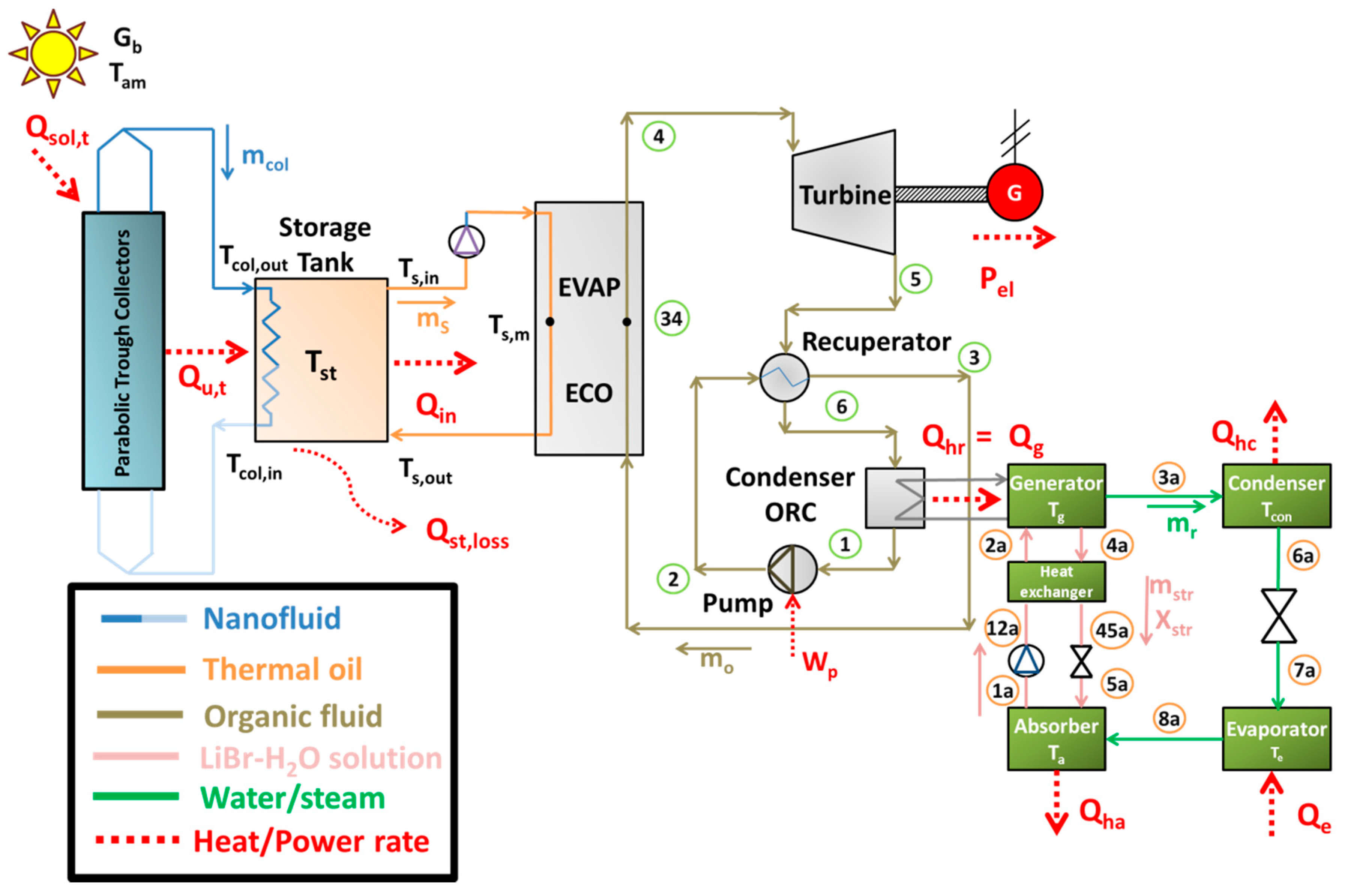
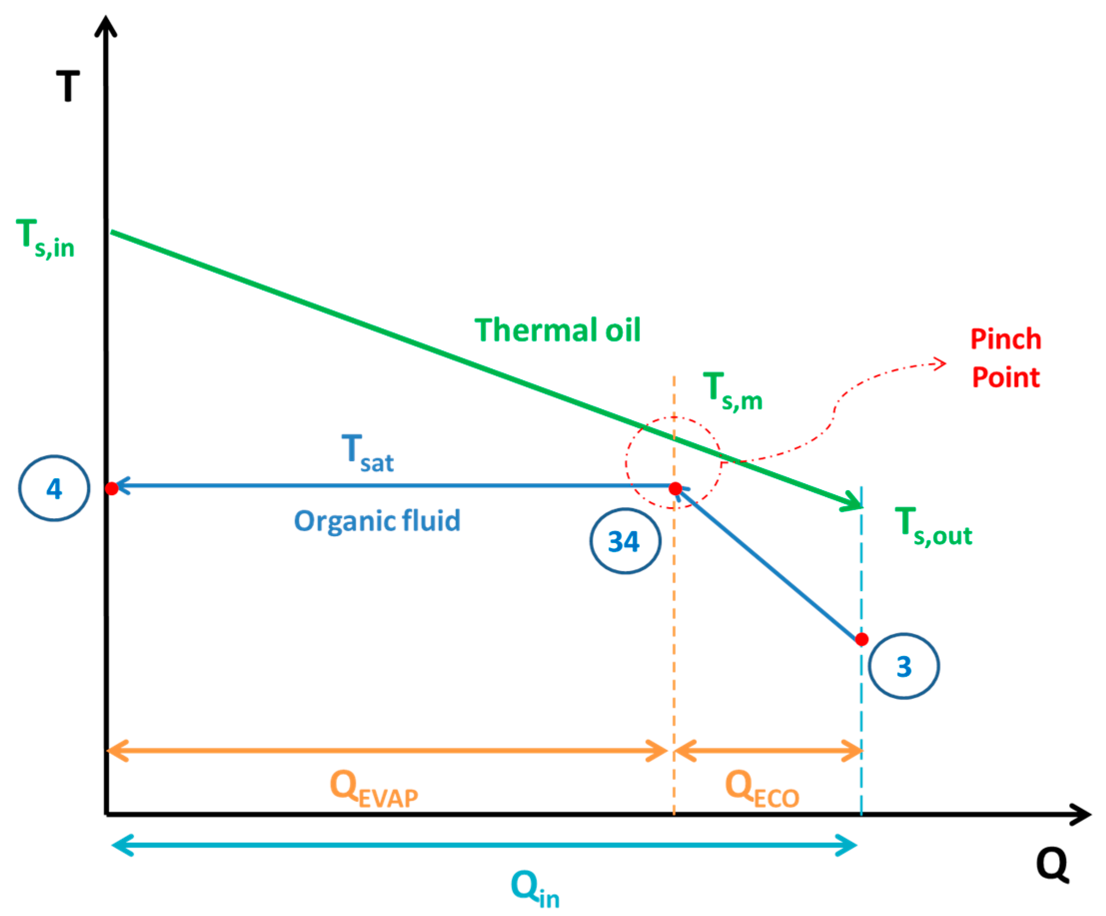
On the other side of the system, heat is transferred to the ORC. Hot thermal oil from the upper part of the storage tank with temperature (
Ts,in) goes to the heat recovery system and heat (
Qin) is transferred in the ORC. The colder thermal oil, in the outlet of the heat recovery system, has a temperature (
Ts,out).
Figure 4 depicts the general heat exchange process inside the storage tank. The pinch point is observed at the start of the evaporator and the temperature of the thermal oil at this point is calculated as:
At this study, the pinch point is taken equal to 10 °C, a typical value according to the literature [
45].
2.3.4. Absorption Heat Pump Modeling
The simulation of the absorption heat pump is performed by using the energy balances in all the circuit devices and the demanded mass flow rate energy balances. The working pair in the absorption cycle is LiBr-H2O and the refrigerant is water/steam. The following Equations (38)–(41) describe the energy balances in the system devices (generator, evaporator, condenser and absorber):
Generator:
Evaporator:
Condenser:
Absorber:
The total heating (
Qh) output of the system is produced both in the condenser and in the absorber:
The mass flow rate balances in the generator are presented by Equations (43)–(44). Equation (43) is the total mass flow rate balance and Equation (44) the mass flow rate energy balance for the LiBr substance. It has been supposed that the outlet of the generator is pure steam without LiBr.
The next important part of the absorption heat pump is the solution heat exchanger. In this device, two are the main equation for its modeling: the energy balance Equation (45) and the heat exchanger effectiveness definition Equation (46):
The throttling valves of the system have been assumed to be adiabatic, fact that makes the enthalpy to be preserved in the expansion in these devices:
Moreover, the work input in the solution pump is neglected as the enthalpy of the state point 12a is calculated as:
Another important point in the present modeling is about the temperature levels in the condenser and in the absorber. These devices reject heat which is utilized for heating proposes. Thus these devices operate under the same temperature levels, in this modeling:
Moreover, the temperature difference between the ORC condenser (heat rejection) and the generator is calculated as:
Also, it is essential to state that all the rejected heat from the ORC condenser is given to the generator of the absorption heat pump:
2.3.5. Definition of System Indexes
In this subsection, various indexes are determined in order to evaluate the performance of the examined system. These indexes concern the subsystems and all the examined system. The electricity efficiency of the ORC (
ηorc) is calculated as:
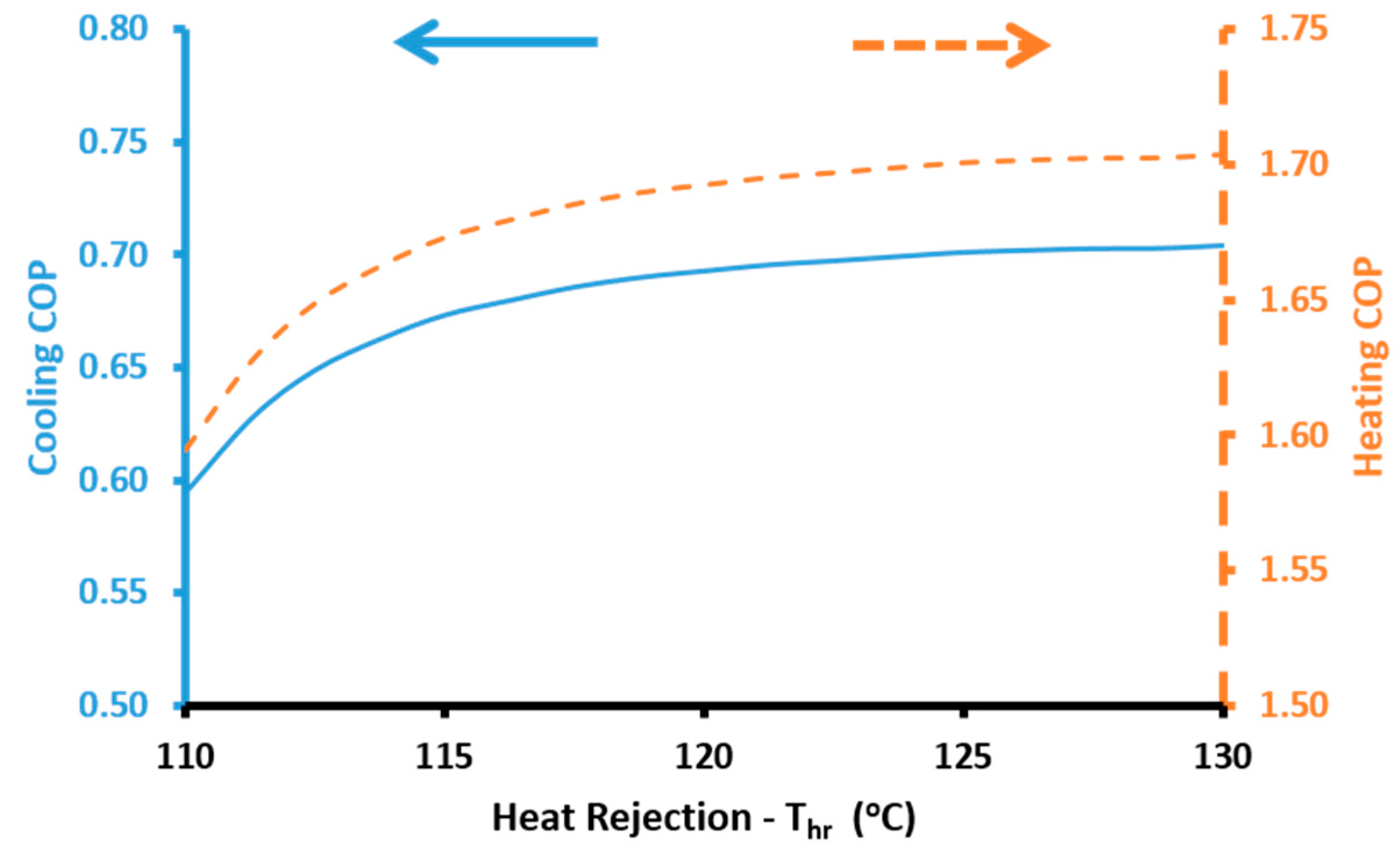
The cooling performance of the absorption heat pump is calculated with the cooling coefficient of performance (
COPcool):
The heating performance of the absorption heat pump is calculated with the heating coefficient of performance (
COPheat):
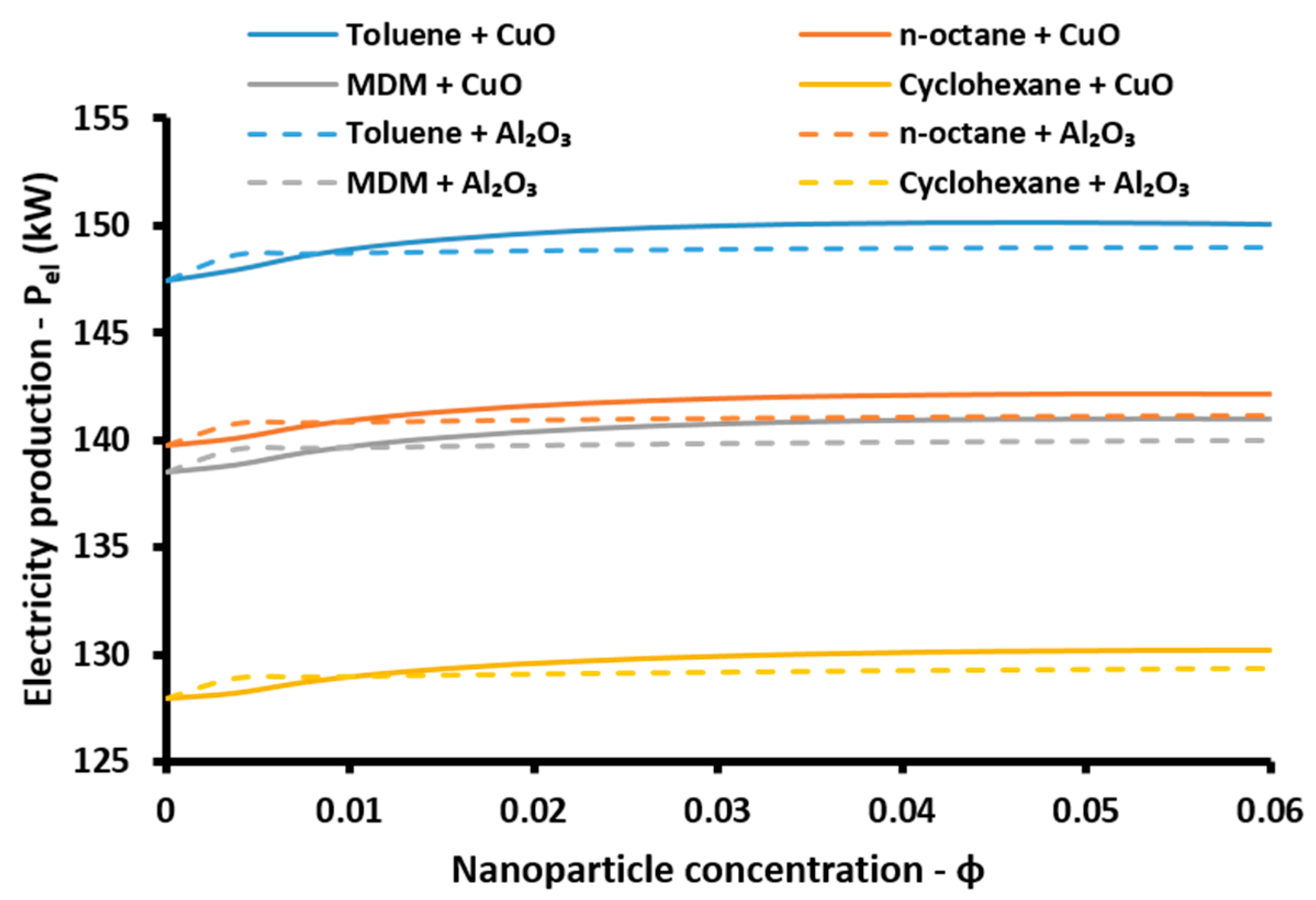
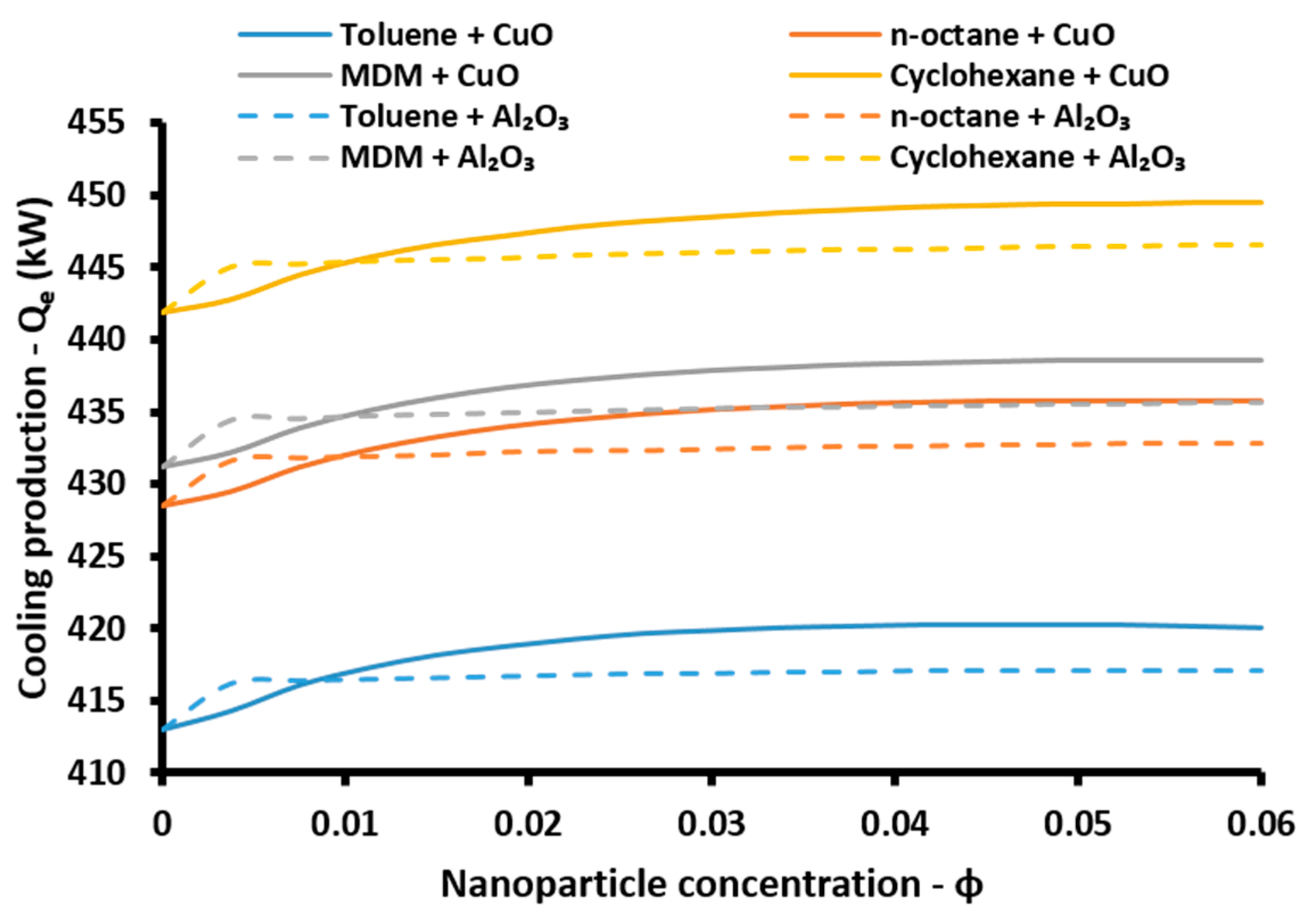
The energetic efficiency of the system is the ratio of the useful energy outputs to the energy input in the system. The useful outputs are the net electricity production (
Pnet), the cooling (
Qe) and the heating (
Qh) loads, while the solar energy is the energy inputs. So, the energetic efficiency (
ηen) is calculated as [
47]:
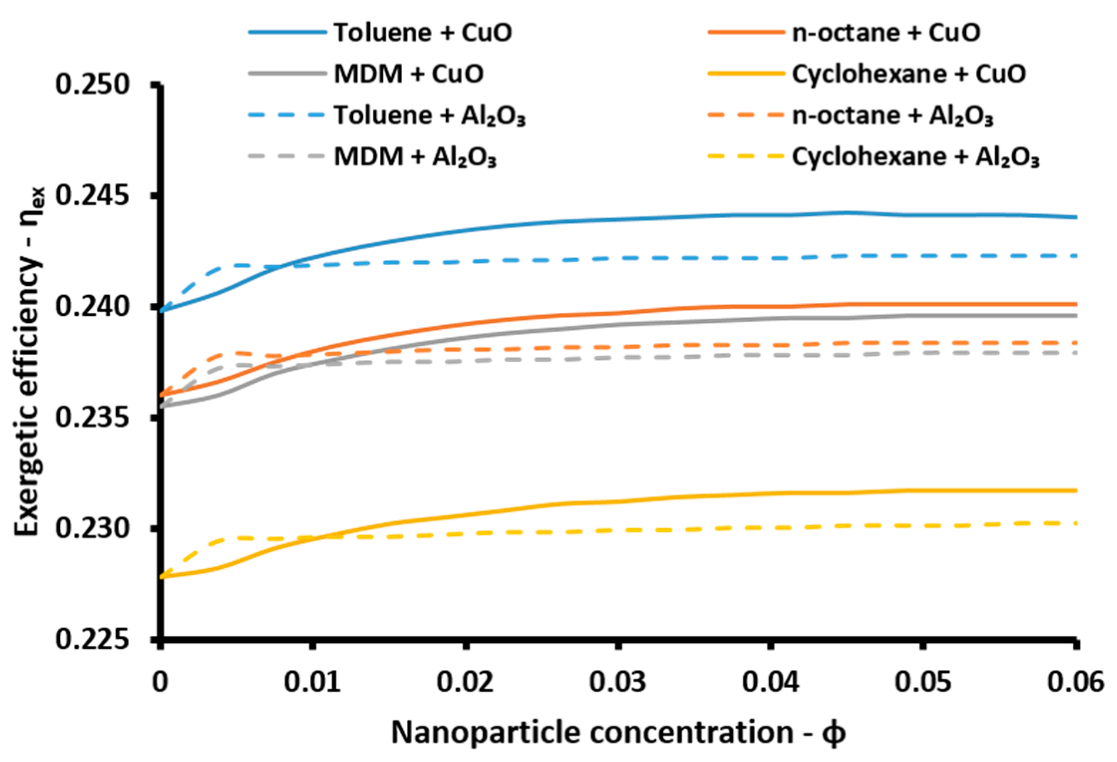
The energetic index can take values over 100% because of the existence of the absorption heat pump. More specifically, this device acts as a heat transformer and the heat output in the absorber and in the condenser have an adequate temperature in order to be exploited. Thus, the sum of all the useful energetic parameters is greater than the solar energy input in the system. This index is a simple index for evaluating the system performance. On the other hand, the exergetic efficiency (
ηex) is a more suitable performance index which takes into consideration the quality of the useful output. This parameter is defined according to Equation (57) [
48]:
The exergy of the solar irradiation (
Esol,t) is estimated by the Petela model Equation (58). The temperature of the sun (
Tsun) is taken equal to 5770 K, a representative value for the outer layer of the sun [
49].


