Numerical Analysis on the Formation of Fracture Network during the Hydraulic Fracturing of Shale with Pre-Existing Fractures

Abstract

In this paper, configurations of pre-existing fractures in cubic rock blocks were investigated and reconstructed for the modeling of experimental hydraulic fracturing. The fluid-rock coupling process of hydraulic fracturing was simulated based on the displacement discontinuities method. The numerical model was validated against the related laboratory experiments. The stimulated fracture configurations under different conditions can be clearly shown using the validated numerical model. First, a dominated fracture along the maximum principle stress direction is always formed when the stress difference is large enough. Second, there are less reopened pre-existing fractures, more newly formed fractures and less shear fractures with the increase of the cohesion value of pre-existing fractures. Third, the length of the stimulated shear fracture decreases rapidly with the increase of the friction coefficient, while the length of the tensile fracture has no correlation to the fiction coefficient. Finally, the increase of the fluid injection rate is favorable to the formation of a fracture network. The unfavorable effects of the large stress difference and the large cohesion of pre-existing fractures can be partly suppressed by an increase of the injection rate in the hydraulic fracturing treatment. The results of this paper are useful for understanding fracture propagation behaviors during the hydraulic fracturing of shale reservoirs with pre-existing fractures.

1. Introduction

Fracture propagation behavior during the hydraulic fracturing treatment of shale reservoirs has been investigated by many researchers. For example, Zoback et al. [1] implemented both laboratory experiments and numerical modeling to demonstrate that the slow slip on pre-existing fractures is important to the effectiveness of slick-water hydraulic fracturing. Nagel et al. [2] found that a higher injection rate favors the creation of tensile failure, while a lower injection rate and lower viscosity favor the creation of shear fracture. Riahi and Damjanac [3] performed a series of comparative studies to establish the effects of injection rates, connectivity, and size distribution of natural fractures on the stimulated area. Fu et al. [4] simulated the fracturing process with dozens of natural fractures to investigate the effects of principal stress orientation and stress anisotropy. McClure and Horne [5] showed that fracturing stimulation may occur through a mixture of the opening and sliding of pre-existing fractures as well as the propagation of new fractures. Zhang and Jeffrey [6] simulated the fracturing process under two injection types and found that constant rate injection is better than constant pressure injection in creating fracture network. Zangeneh et al. [7] investigated the relationship between hydraulic fracturing and triggering of fracture slip of a rock mass with pre-existing fractures. Aside from the works listed above, fracture propagation behaviors during the hydraulic fracturing treatment have also been investigated by many other researchers [8,9,10,11,12,13,14]. Pre-existing fractures in the rock play an important role in the formation of the fracture network during hydraulic fracturing. For typical continental sedimentary shale in China, pre-existing fractures on a small scale are also very important. For example, small-scale pre-existing fractures are well developed in the Upper Triassic Yanchang formation of Ordos Basin [15]. Zhou et al. [16] conducted laboratory experiments to investigate fracture propagation based on these pre-existing fractures. However, as experiments are difficult to carry out and the comparability is poor, Zhou et al. [16] only studied the effects of stress difference on fracture propagation.

Compared with laboratory experiments, numerical modeling is much more flexible and can be used in more complicated cases. However, numerical modeling is very challenging as the propagation of fracture networks depends on many factors, such as pre-existing fractures, rock properties, in situ stress, fluid properties, and injection rate. Many methods have been developed to simulate the fluid-rock coupling process of hydraulic fracturing, including the finite element method [17], extended finite element method [18], discrete element method [4], and mesh-less method [1,19,20,21,22,23]. Precision and efficiency are crucially important to the modeling of the hydraulic fracturing process. As the simulation domain is often hundreds of meters, whereas the typical fracture aperture is a small fraction of a millimeter, a deformation that is considered as small “noise” in the solid solver may induce dramatic oscillation of fluid pressure in the flow solver [4]. The Displacement Discontinuity Method (DDM) [24] is another novel method for modeling the fluid-rock coupling system of hydraulic fracturing. In this method, fracture displacement discontinuities can be calculated with higher precision because the analytical solution is directly used to calculate the induced stress. IN addition, the fracturing process can be simulated with very high computational efficiency as the grid number is much less than that used in other methods because the rock matrix is not discretized in DDM. The propagation of a complex fracture network with hundreds of fractures can be easily simulated using DDM [9,11,14,25,26,27].

In this study, the propagation behavior of fractures during hydraulic fracturing of rock with pre-existing fractures is investigated with a newly proposed numerical model based on DDM. This approach offers a preliminary understanding of the formation of the fracture network during hydraulic fracturing of a shale reservoir with pre-existing fractures. First, the numerical model is set up and validated against laboratory experiments. Then, using the validated numerical model, multi-factor analyses are carried out to investigate the propagation of fractures under different conditions during the hydraulic fracturing process.

2. Numerical Method

A DDM-based model is used to simulate the hydraulic fracturing process in this study. The following assumptions are used in the model: the rock matrix is homogeneous, isotropous, and linear elastic [24]. The rock matrix is impermeable. The fluid injected is Newtonian, single phase, and laminar [6,25,28]. The details of the model had been introduced in our previous published papers [13] therefore, for the sake of completeness, only the most important equations are given blow.

Given the normal and shear Displacement Discontinuities (DDs) of each fracture element, the induced stresses by the opening and sliding of the fracture system with N elements can be calculated by [6]:

$$\begin{array}{l}{\sigma }_n\left(x\right)={\displaystyle \sum _{r=1}^N{\displaystyle {\int }_0^{l_r}\left[G_{11}\left(x,s\right)w\left(s\right)+G_{12}\left(x,s\right)\nu \left(s\right)\right]K\left(x,s\right)ds}}\\ {\tau }_s\left(x\right)={\displaystyle \sum _{r=1}^N{\displaystyle {\int }_0^{l_r}\left[G_{21}\left(x,s\right)w\left(s\right)+G_{22}\left(x,s\right)\nu \left(s\right)\right]K\left(x,s\right)ds}}\end{array}$$

(1)

where x = (x, y) is the coordinate, w is the normal DD, v is the shear DD, l_r is the length of fracture, r, G_ij are the hyper singular Green’s functions, which are proportional to the plane strain Young’s modulus [6], σ_n is the normal stress, and τ_s is the shear stress, obeying Coulomb’s frictional law characterized by the coefficient of friction λ, which limits the shear stress by:

$$\left|{\tau }_s\right|\le \lambda {\sigma }_n$$

(2)

that can act in parts of fractures that are in contact, but vanishes along the separated parts. Along the opened fracture portions, we have:

$${\sigma }_n=p_f$$

(3)

where K is the three-dimensional correction coefficient proposed by Olson [29].

The fracture growth is based on the maximum hoop stress criterion, with the maximum mixed-mode intensity factor reaching a critical value at:

$$\frac{1}{2}\cos \frac{{\theta }_0}{2}\left[K_I\left(1+\cos {\theta }_0\right)-3K_{II}\sin {\theta }_0\right]=K_{IC}$$

(4)

where K_I and K_II are stress intensity factors, K_IC is the tensile mode fracture toughness, and $\theta$ is the fracture propagation direction relative to the current fracture orientation, and satisfies:

$$K_I\sin \theta +K_{II}\left(3\cos \theta -1\right)=0$$

(5)

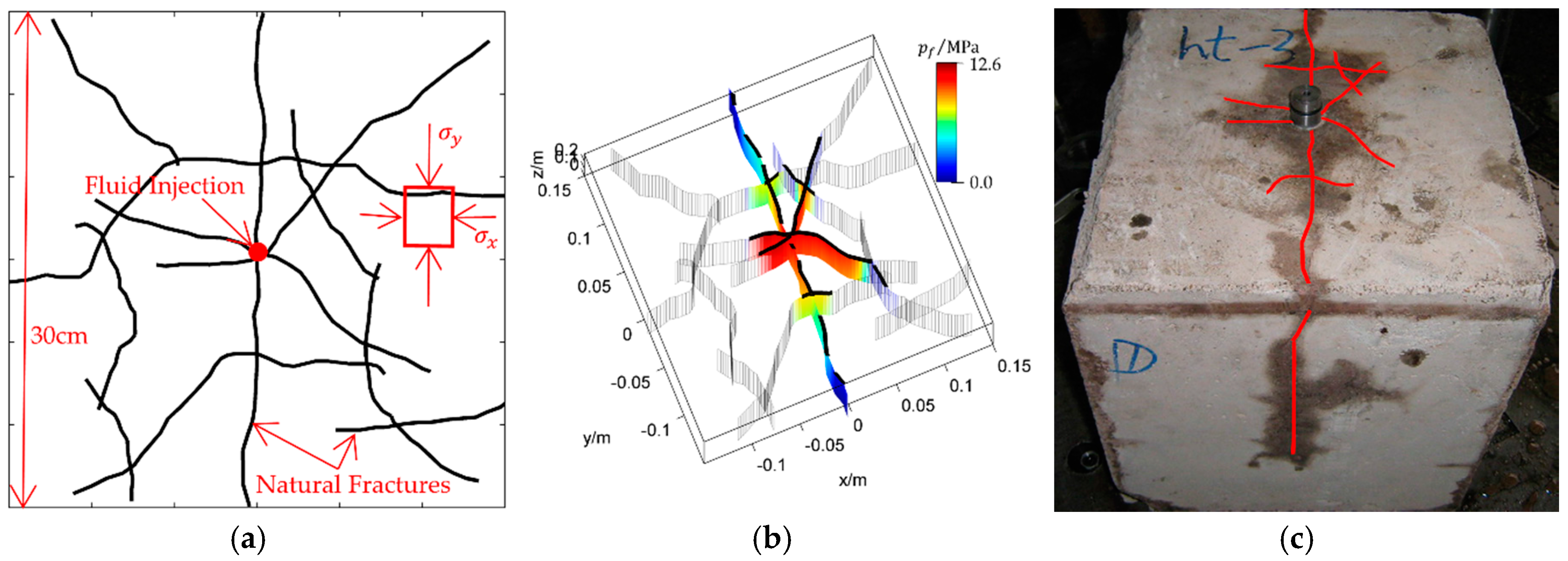
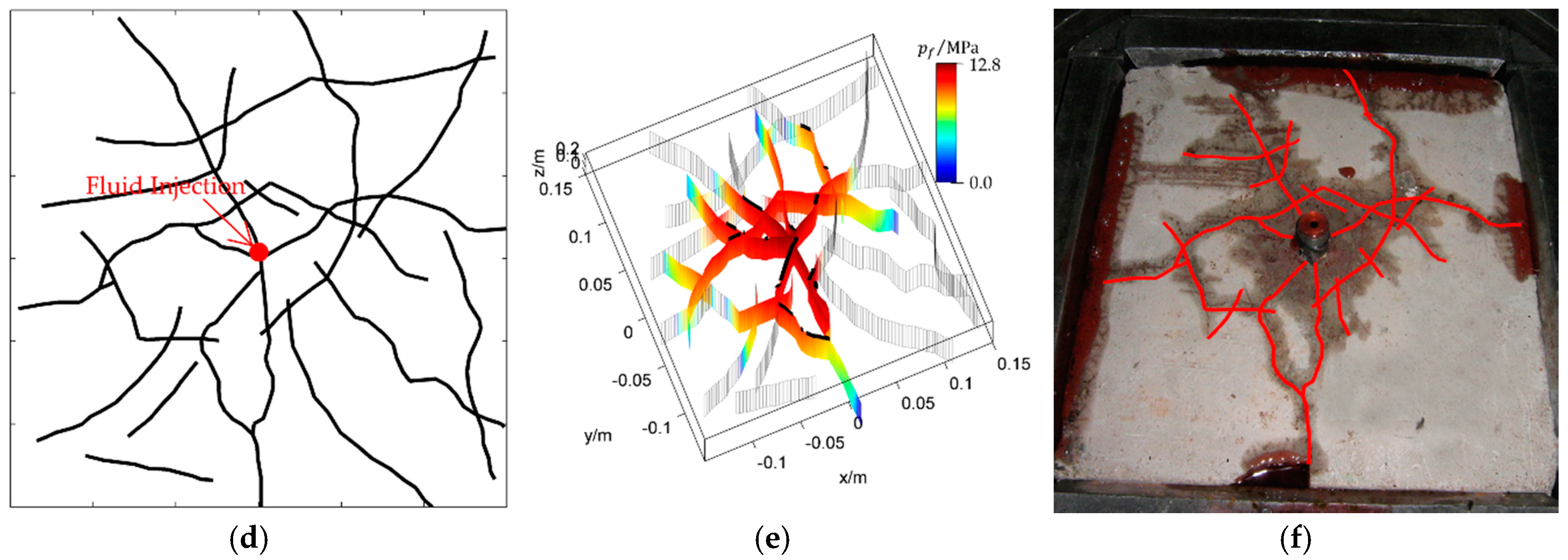
3. Model Setup and Model Validation

The pre-existing fractures were reconstructed based on the results of the laboratory experiments implemented by Zhou et al. [16]. After the repeated heating and cooling processes for cement blocks, the random pre-existing fractures as shown in Figure 1 were obtained. These pre-existing fractures were then identified from the gray scale images of the cement blocks by using a gray threshold value. The identified pre-existing fractures are shown in Figure 2a,d.

The hydraulic fracturing processes were then simulated by injecting fluid from the central position of the numerical model. The model setup is illustrated in Figure 2a. The fractures propagate from the center with the fluid injection from the central position. The modeling is finished when any fracture reaches the boundary of the region.

To validate the model, two numerical tests were implemented according to the laboratory experiments conducted by Zhou et al. [16]. All of the default parameters are listed in

Table 1. Default input parameters for the simulations in this paper. Here, ${\sigma }_x$ and ${\sigma }_y$ are the principle stresses along the x and y-axis directions respectively, $\lambda$ is the friction coefficient between fracture surfaces, C is the cohesion of pre-existing fractures, layer thickness is the height of the model perpendicular to the modeling plain, and K_IC is tensile mode fracture toughness.

Parameter	Value	Parameter	Value
Young’s Modulus	8.4 GPa	Poisson’s ratio	0.23
Fluid Viscosity	135 mPa.s	Injection Rate	13.9 × 10−3 m2/s
${\sigma }_x$	1 MPa	${\sigma }_y-{\sigma }_x$	0 MPa
$\lambda$	0.9	C	0 MPa
Layer Thickness	0.3 m	KIC	1.0 MPa·m0.5

. These parameters are equivalent to those used by Zhou et al. [16] and are used as default in all the simulations in this work. For case 1, the hydraulic fracturing process is simulated under a high stress difference (${\sigma }_y-{\sigma }_x=10 \mathrm{MPa}$) based on the pre-existing fracture network as shown in Figure 2a. For case 2, the hydraulic fracturing process is simulated under a small stress difference (${\sigma }_y-{\sigma }_x=5 \mathrm{MPa}$) based on the pre-existing fracture network as shown in Figure 2d. The numerical results of the two cases are shown in Figure 2b,e. Vertical dominated fractures with multiple branches are formed under a high stress difference while a radial fracture system is formed under a small stress difference. The numerical results agree well with the experiment results that are shown in Figure 2c,f.

It must be noted that it is difficult to control the mechanical properties of pre-existing fractures (e.g., friction coefficient, cohesion, etc.) in the laboratory experiments. Moreover, as a rock sample can only be hydraulic fractured once, it is impossible to investigate the fracture network propagation based on the same pre-existing fracture network under different conditions. Fortunately, the numerical modeling method provides us a really feasible solution. We are able to investigate the propagation of a fracture network under more complex situations through numerical modeling based on the second pre-existing fracture configuration, as shown in Figure 2d in the following sections.

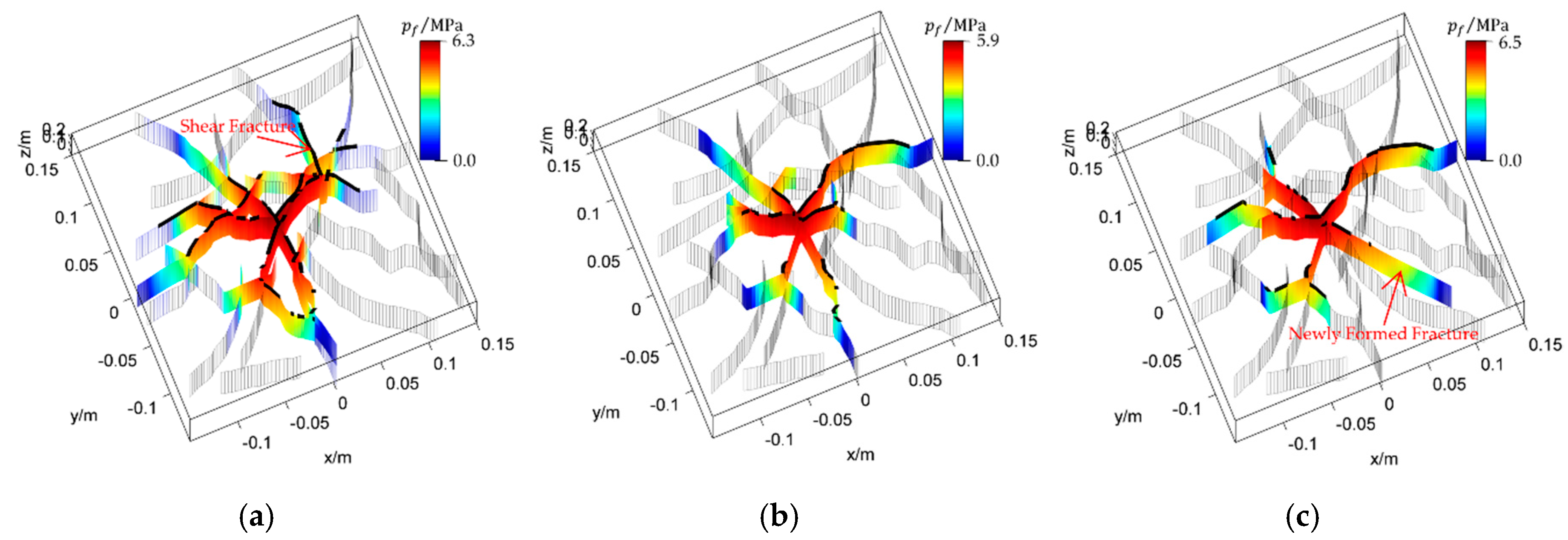
4. Results and Discussion

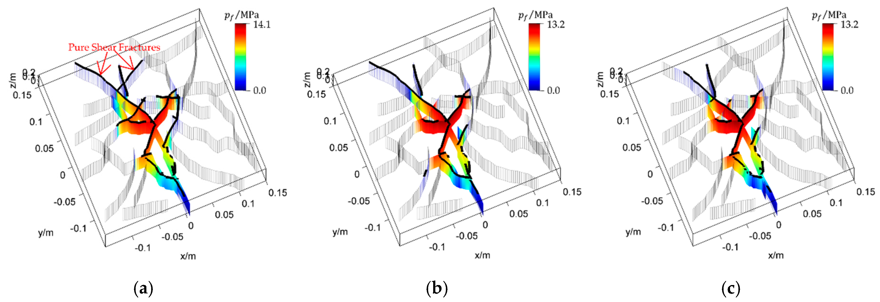
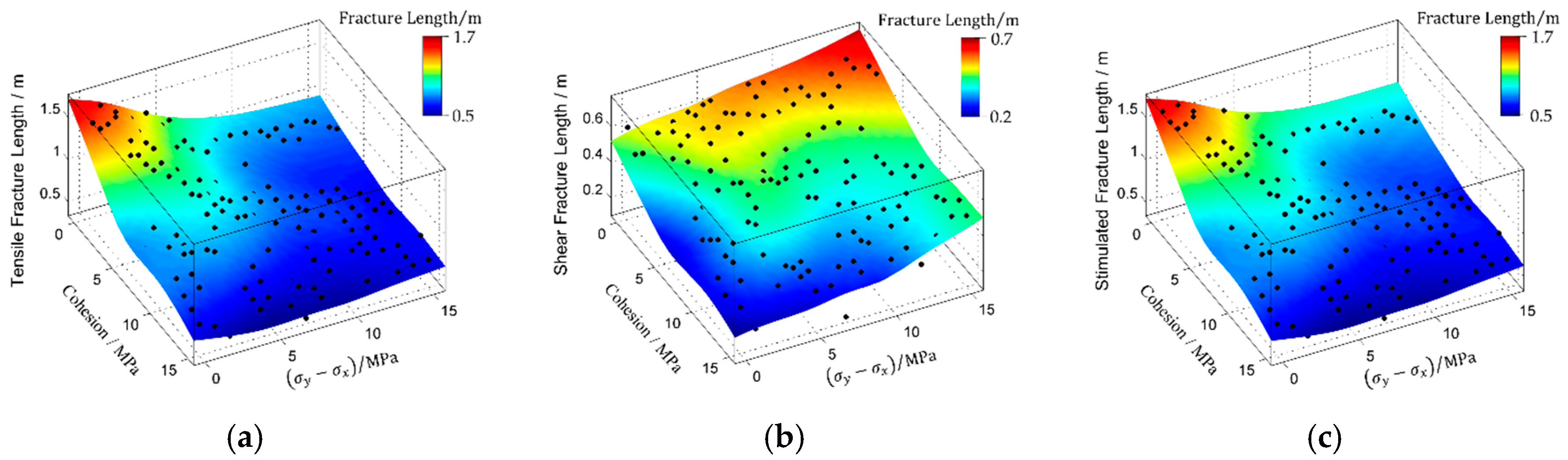
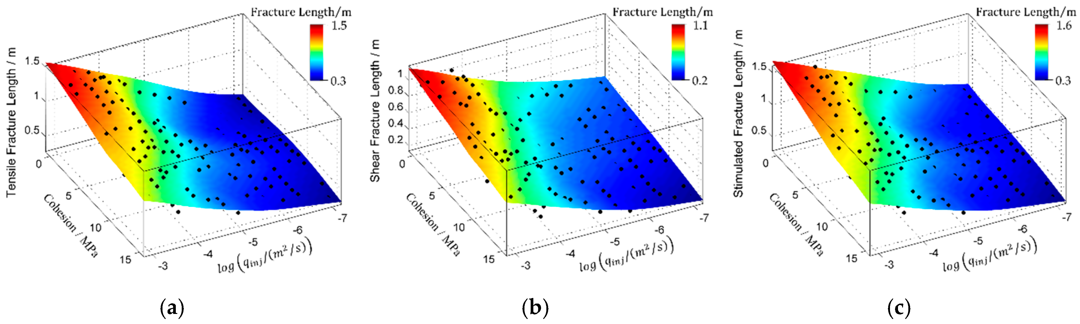
4.1. Effects of The Cohesion of Pre-Existing Fractures

As the aperture of pre-existing fractures is in the range of 0.05–0.1 mm in the research conducted by Zhou et al. [16], the cohesion of pre-existing fractures can be treated as ignorable in the simulations above. However, for shale reservoirs, the aperture of pre-existing fractures is much smaller than that in Zhou et al. [16] and thus the cohesion of pre-existing fractures is always pertinent. In this section, the effects of cohesion on fracture propagation are investigated.

The cohesion of pre-existing fractures has great effects on fracture network propagation, as shown in Figure 3. Firstly, when the cohesion is greater, there are less reopened pre-existing fractures because more energy is needed to reopen such pre-existing fractures. Secondly, when the cohesion is greater, there are more newly formed hydraulic fractures because there is less fluid flow through the pre-existing fractures. Thirdly, the final fracture network configuration is less complex when the cohesion is larger. This indicates that, with the increasing of cohesion, the increasing of the newly formed fracture length is slower than the decreasing of the reopened pre-existing fracture length. Finally, there is less shear fractures when the cohesion is greater. This can be explained by the maximum hoop stress criterion, according to which a newly formed hydraulic fracture will change the propagation direction when the shear stress along the fracture is not equal to zero.

To show the effects of cohesion more clearly, the variations of the fracture lengths with cohesion and stress difference are illustrated in Figure 4. Here, the tensile fracture is defined as a fracture that is filled by fluid, the shear fracture is defined as a fracture with a shear displacement discontinuity greater than 10$\mathsf{\mu }\mathrm{m}$, and the stimulated fracture is defined as a fracture that is either a tensile or shear fracture. It can be seen that all of these fracture lengths decrease with the increasing of cohesion. However, the variation sensitivities are much different. First, when the stress difference is small, the tensile fracture length decreases rapidly with the increasing of cohesion. By contrast, the shear fracture length is not very sensitive to the increasing of cohesion when the stress difference is relatively large. This is caused by the fact that the shear stimulation is not very significant when the stress difference is small. Second, when the stress difference is large, the shear fracture length decreases rapidly with the increasing of cohesion, but the decreasing of the tensile fracture length is not very significant. This can be explained by the fracture network propagation behavior when the stress difference is large. As illustrated in Section 3, the fracture network propagates mainly along the maximum principle stress direction. Moreover, when the stress difference is large, the fracture propagation behavior is controlled by the stress difference. As a result, a dominated fracture is always formed and thus the affected fracture length is not as sensitive to the cohesion increasing when the stress difference is large.

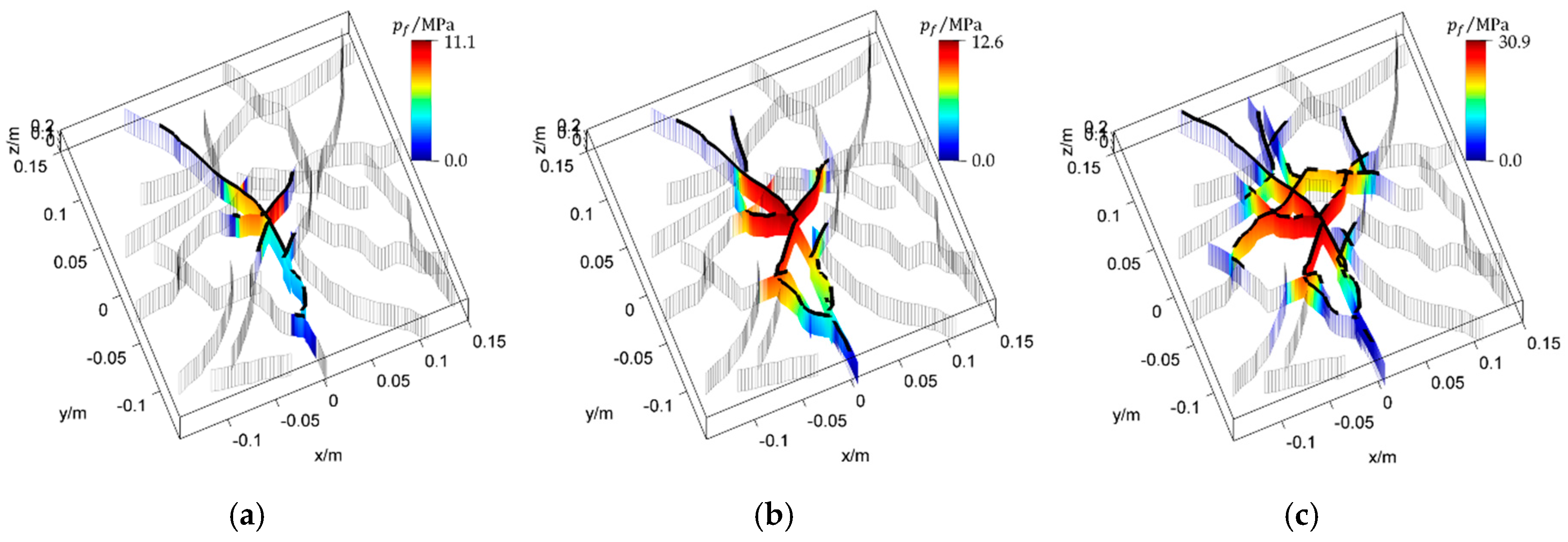
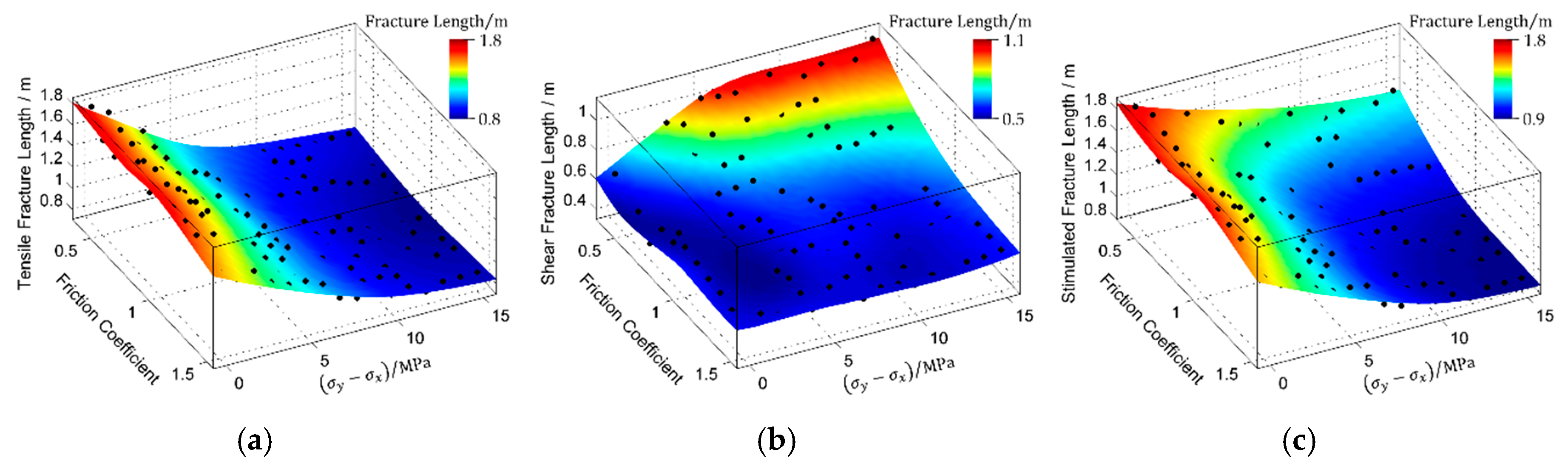
4.2. Effects of the Friction Coefficient

Aside from the cohesion of pre-existing fractures, the friction coefficient is also an important fracture characteristic. In this section, the effects of the friction coefficient are investigated. The fracture network configurations under different friction coefficients are shown in Figure 5. It can be seen that the fracture network is comparable under different friction coefficients. However, the effects of the friction coefficient is important. A pre-existing fracture is more difficult to be reopened when the friction coefficient is larger. Comparing Figure 5c with Figure 5a, it is found that the pure shear stimulated fractures, which are the fractures that are shear stimulated before being filled with fluid, are much shorter when the friction coefficient is greater.

The variations of fracture lengths with the friction coefficient and stress difference are shown in Figure 6. It can be seen that the friction coefficient has ignorable effects on tensile fractures under both low and high stress differences. This agrees well with the fracture network configurations that are shown in Figure 5. Although different from the tensile fractures, the shear fracture length varies sensitively with the friction coefficient, especially when the stress difference is large. Upon increasing the friction coefficient, there are much less pre-existing fractures reopened by shear stimulation. Therefore, the shear fracture length decreases with the increasing of the friction coefficient. In summary, the friction coefficient between fracture surfaces has great effects on the propagation of shear fractures but has ignorable effects on tensile fractures.

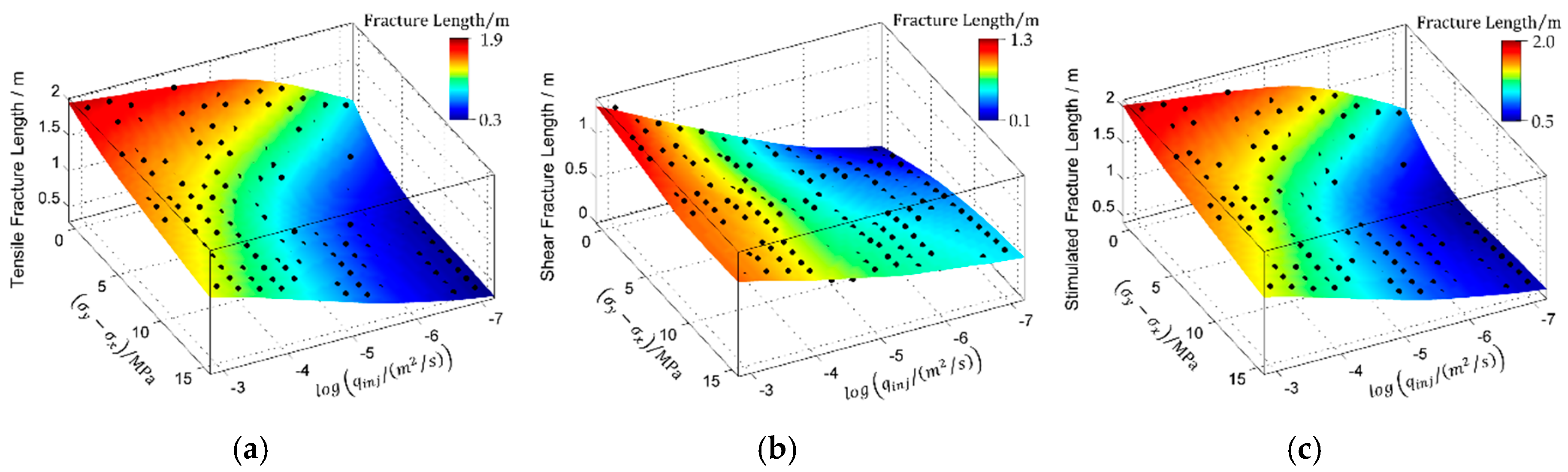
4.3. Effects of the Injection Rate

Injection rate is one of the most important operating parameters during the hydraulic fracturing treatment of shale reservoirs. Fracture network configurations under different injection rates are shown in Figure 7. The maximum principle stress direction is along the y-axis direction and the stress difference is 10 MPa in these simulations. The fracture network propagates mainly along the maximum principle stress direction (y-axis direction), and dominated hydraulic fractures are formed when the injection rate is low. However, the fracture network also propagate along the x-axis direction when the injection is high. Comparing these fracture network configurations in Figure 7, it is clear that the fracture network is more complex when the injection rate is higher.

The variations of the fracture lengths with the injection rate and stress difference are shown in Figure 8. The fracture lengths increase with the increasing injection rate under both isotropous and anisotropic crustal stress conditions. However, the increasing of the injection rate is more significant to the formation of the fracture network when the stress difference is large. The affected fracture length decreases with the increasing of stress difference when the injection rate is low. However, the unfavorable effects of stress difference can be partly suppressed by the increasing of the injection rate. Both the tensile and shear fracture lengths increase with the increasing of the injection rate. The variations of the fracture lengths with the injection rate and the cohesion of pre-existing fractures are also simulated, and the results are shown in Figure 9. The fracture lengths decrease with the increasing of cohesion and increase with the increasing of the injection rate. To sum up, the increasing of the injection rate is favorable to the formation of the fracture network.

5. Conclusions

The formation of the fracture network during hydraulic fracturing of reservoir rock with pre-existing fractures is investigated using a numerical model based on the displacement discontinuities method. The numerical modeling is carried out based on the reconstruction of the pre-existing fracture networks generated from repeated heating and cooling processes in cubic rock blocks. The numerical results are validated by the laboratory experiments. The fracture network configurations under different conditions are obtained by the validated numerical model.

Firstly, the increasing of stress difference is unfavorable to the formation of the fracture network as a dominated fracture along the maximum principle stress direction could be formed when the stress difference is large. However, a larger stress difference is favorable to the shear stimulation. Secondly, the high cohesion of pre-existing fractures is also unfavorable to the formation of the fracture network as the reopening of pre-existing fractures could be suppressed by the larger cohesion. Moreover, there are less shear fractures when the cohesion is larger. Thirdly, shear stimulation could be suppressed by the greater friction coefficient between fracture surfaces, but the tensile mode fractures are not affected by the friction coefficient. Moreover, fracture propagation is related to the friction coefficient mainly when the anisotropy of stress is strong. Finally, increasing the injection rate is favorable to the formation of the fracture network under different stress differences and different cohesions of pre-existing fractures. Upon increasing the injection rate, the lengths of both the tensile and the shear mode fractures increase.

References

1. Zoback, M.D.; Kohli, A.; Das, I.; McClure, M.W. The importance of slow slip on faults during hydraulic fracturing stimulation of shale gas reservoirs. In Proceedings of the Americas Unconventional Resources Conference, Pittsburgh, PA, USA, 5–7 June 2012; Society of Petroleum Engineers: Richardson, TX, USA, 2012. [Google Scholar]
2. Nagel, N.B.; Gil, I.; Sanchez-nagel, M.; Damjanac, B. Simulating hydraulic fracturing in real fractured rocks—Overcoming the limits of pseudo3d models. In Proceedings of the SPE Hydraulic Fracturing Technology Conference and Exhibition, The Woodlands, TX, USA, 24–26 January 2011; Society of Petroleum Engineers: Richardson, TX, USA, 2012. [Google Scholar]
3. Riahi, A.; Damjanac, B. Numerical study of interaction between hydraulic fracture and discrete fracture network. In Proceedings of the ISRM International Conference for Effective and Sustainable Hydraulic Fracturing, Brisbane, Australia, 20–22 May 2013. [Google Scholar]
4. Fu, P.C.; Johnson, S.M.; Carrigan, C.R. An explicitly coupled hydro-geomechanical model for simulating hydraulic fracturing in arbitrary discrete fracture networks. Int. J. Numer. Anal. Methods Géoméch. 2013, 37, 2278–2300. [Google Scholar] [CrossRef]
5. McClure, M.W.; Horne, R.N. Conditions required for shear stimulation in egs. In Proceedings of the 2013 European Geothermal Congress, Pisa, Italy, 19–14 September 2013. [Google Scholar]
6. Zhang, X.; Jeffrey, R. Development of fracture networks through hydraulic fracture growth in naturally fractured reservoirs. In Proceedings of the ISRM International Conference for Effective and Sustainable Hydraulic Fracturing, Brisbane, Australia, 20–22 May 2013. [Google Scholar]
7. Zangeneh, N.; Eberhardt, E.; Marc, R.; Busti, A. A numerical investigation of fault slip triggered by hydraulic fracturing. In Proceedings of the ISRM International Conference for Effective and Sustainable Hydraulic Fracturing, Brisbane, Australia, 20–22 May 2013. [Google Scholar]
8. Olson, J.E. Multi-fracture propagation modeling: Applications to hydraulic fracturing in shales and tight gas sands. In Proceedings of the 42nd U.S. Rock Mechanics Symposium and 2nd U.S.-Canada Rock Mechanics Symposium, San Francisco, CA, USA, 29 June–2 July 2008. [Google Scholar]
9. Kresse, O.; Weng, X.W.; Gu, H.R.; Wu, R.T. Numerical modeling of hydraulic fractures interaction in complex naturally fractured formations. Rock Mech. Rock Eng. 2013, 46, 555–568. [Google Scholar] [CrossRef]
10. Wu, K.; Olson, J.E. Simultaneous multifracture treatments: Fully coupled fluid flow and fracture mechanics for horizontal wells. SPE J. 2015. [Google Scholar] [CrossRef]
11. Weng, X. Modeling of complex hydraulic fractures in naturally fractured formation. J. Unconv. Oil Gas Resour. 2015, 9, 114–135. [Google Scholar] [CrossRef]
12. Zhuang, X.; Huang, R.; Liang, C.; Rabczuk, T. A coupled thermo-hydro-mechanical model of jointed hard rock for compressed air energy storage. Math. Probl. Eng. 2014, 2014, 179169. [Google Scholar] [CrossRef]
13. Zhang, Z.; Li, X. Numerical study on the formation of shear fracture network. Energies 2016, 9, 299. [Google Scholar] [CrossRef]
14. Zhang, Z.; Li, X.; He, J.; Wu, Y.; Zhang, B. Numerical analysis on the stability of hydraulic fracture propagation. Energies 2015, 8, 9860–9877. [Google Scholar] [CrossRef]
15. Tang, X.; Zhang, J.C.; Wang, X.Z.; Yu, B.S.; Ding, W.L.; Xiong, J.Y.; Yang, Y.T.; Wang, L.; Yang, C. Shale characteristics in the southeastern Ordos basin, China: Implications for hydrocarbon accumulation conditions and the potential of continental shales. Int. J. Coal Geol. 2014, 128, 32–46. [Google Scholar] [CrossRef]
16. Zhou, J.; Jin, Y.; Chen, M. Experimental investigation of hydraulic fracturing in random naturally fractured blocks. Int. J. Rock Mech. Min. Sci. 2010, 47, 1193–1199. [Google Scholar] [CrossRef]
17. Rahman, M.M.; Rahman, S.S. Studies of hydraulic fracture-propagation behavior in presence of natural fractures: Fully coupled fractured-reservoir modeling in poroelastic environments. Int. J. Geomech. 2013, 13, 809–826. [Google Scholar] [CrossRef]
18. Mohammadnejad, T.; Khoei, A.R. An extended finite element method for fluid flow in partially saturated porous media with weak discontinuities; the convergence analysis of local enrichment strategies. Comput. Mech. 2013, 51, 327–345. [Google Scholar] [CrossRef]
19. Rabczuk, T.; Gracie, R.; Song, J.H.; Belytschko, T. Immersed particle method for fluid–structure interaction. Int. J. Numer. Methods Eng. 2010, 81, 48–71. [Google Scholar] [CrossRef]
20. Zhuang, X.; Augarde, C.; Mathisen, K. Fracture modeling using meshless methods and level sets in 3d: Framework and modeling. Int. J. Numer. Methods Eng. 2012, 92, 969–998. [Google Scholar] [CrossRef]
21. Zhuang, X.; Cai, Y.; Augarde, C. A meshless sub-region radial point interpolation method for accurate calculation of crack tip fields. Theor. Appl. Fract. Mech. 2014, 69, 118–125. [Google Scholar] [CrossRef]
22. Rabczuk, T.; Belytschko, T. A three-dimensional large deformation meshfree method for arbitrary evolving cracks. Comput. Methods Appl. Mech. Eng. 2007, 196, 2777–2799. [Google Scholar] [CrossRef]
23. Rabczuk, T.; Belytschko, T. Cracking particles: A simplified meshfree method for arbitrary evolving cracks. Int. J. Numer. Methods Eng. 2004, 61, 2316–2343. [Google Scholar] [CrossRef]
24. Crouch, S.L.; Starfield, A.M. Boundary Element Methods in Solid Mechanics; George Allen & Unwin: London, UK, 1983. [Google Scholar]
25. McClure, M.; Horne, R. Characterizing hydraulic fracturing with a tendency-for-shear-stimulation test. In Proceedings of the SPE Annual Technical Conference and Exhibition, Amsterdam, The Netherlands, 27–29 October 2014. [Google Scholar]
26. Sesetty, V.; Ghassemi, A. Numerical simulation of sequential and simultaneous hydraulic fracturing. In Proceedings of the ISRM International Conference for Effective and Sustainable Hydraulic Fracturing, Brisbane, Australia, 20–22 May 2013. [Google Scholar]
27. Safari, R.; Ghassemi, A. 3d thermo-poroelastic analysis of fracture network deformation and induced micro-seismicity in enhanced geothermal systems. Geothermics 2015, 58, 1–14. [Google Scholar] [CrossRef]
28. Weng, X.; Kresse, O.; Cohen, C.; Wu, R.; Gu, H. Modeling of hydraulic-fracture-network propagation in a naturally fractured formation. SPE Prod. Oper. 2011, 26, 368–380. [Google Scholar] [CrossRef]
29. Olson, J.E. Predicting fracture swarms—the influence of subcritical crackgrowth and the crack-tip process zone on joint spacing in rock. In The Initiation, Propagation, and Arrest of Joints and Other Fractures; Geological Society of London Special Publication: London, UK, 2004; Volume 231, pp. 73–87. [Google Scholar]
Figure 1. Pre-existing fractures on the surface of a block after heat and cooling treatments from Zhou et al. [16].
Energies 10 00736 g001
Figure 2. Fracture network configurations under different stress conditions. (a) The numerical setting and the pre-existing fracture network of case 1; (b) The numerical result of case 1; (c) The experiment result of case 1; (d) The pre-existing fracture network of case 2; (e) The numerical result of case 2; (f) The experiment result of case 2. The pre-existing fracture networks and the experiment results are obtained from Zhou et al. [16]. For numerical results, the fluid pressure (pf) is represented by color. The fractures that are not affected by fluid are represented by the gray meshes. The shear fractures are marked by the bold curves at the top. For experiment results, the stimulated fractures are marked by the bold red curves.
Energies 10 00736 g002aEnergies 10 00736 g002b
Figure 3. Fracture network configurations under different cohesions of pre-existing fracture. (a) C = 0 MPa; (b) C = 5 MPa; (c) C = 10 MPa. Here, C is the cohesion of pre-existing fractures. In these figures, the fluid pressure (pf) in the fluid-affected fractures is represented by color. The fractures that are not affected by fluid are represented by the gray meshes. The shear fractures are marked by the bold curves at the top. The stress difference σ y σ x is equal to 0 MPa in these simulations.
Energies 10 00736 g003
Figure 4. Variations of fracture lengths with stress difference and the cohesion of pre-existing fractures. (a) The variation of the tensile fracture length; (b) The variation of the shear fracture length; (c) The variation of the stimulated fracture length, i.e., the length of the fractures that are either tensile or shear fractures. In these figures, each black point represents the result of a simulation. The colored surfaces represent the smoothed results.
Energies 10 00736 g004
Figure 5. Fracture network configurations under different values of the friction coefficient. (a) λ = 0.4 ; (b) λ = 0.7 ; (c) λ = 1.0 . Here, λ refers to the friction coefficient between fracture surfaces. For the fluid-affected fractures, the fluid pressure (pf) is represented by color. The fractures that are not affected by fluid are represented by the gray meshes. The shear fractures are marked by the bold curves at the top. The stress difference σ y σ x is equal to 10 MPa in these simulations.
Energies 10 00736 g005
Figure 6. Variations of fracture lengths with stress difference and the friction coefficient between fracture surfaces. (a) The variation of the tensile fracture length; (b) The variation of the shear fracture length; (c) The variation of the stimulated fracture length, i.e., the length of the fractures that are either tensile or shear fractures. In these figures, each black point represents the result of a simulation. The colored surfaces represent the smoothed results.
Energies 10 00736 g006
Figure 7. Final fracture network configurations under different injection rates. (a) qinj = 1.0 × 10⁷ m2/s; (b) qinj = 1.0 × 10⁵ m2/s; (c) qinj = 1.0 × 10³ m2/s. For the fluid-affected fractures, the fluid pressure (pf) is represented by color. The fractures that are not affected by fluid are represented by the gray meshes. The shear fractures are marked by the bold curves at the top. The stress difference σ y σ x is equal to 10 MPa in these simulations.
Energies 10 00736 g007
Figure 8. Variations of the fracture lengths with the injection rate and stress difference. (a) The variation of the tensile fracture length; (b) The variation of the shear fracture length; (c) The variation of the stimulated fracture length, i.e., the length of the fractures that are either tensile or shear fractures. In these figures, each black point represents the result of a simulation. The colored surfaces represent the smoothed results.
Energies 10 00736 g008
Figure 9. Variations of the fracture lengths with injection rate and the cohesion of pre-existing fractures. (a) The variation of the tensile fracture length; (b) The variation of the shear fracture length; (c) The variation of the stimulated fracture length, i.e., the length of the fractures that are either tensile or shear fractures. In these figures, each black point represents the result of a simulation. The colored surfaces represent the smoothed results.
Energies 10 00736 g009