Abstract
Photovoltaic (PV) system output electricity is related to PV cells’ conditions, with the PV faults decreasing the efficiency of the PV system and even causing a possible source of fire. In industrial production, PV fault detection is typically laborious manual work. In this paper, we present a method that can automatically detect PV faults. Based on the observation that different faults will have different impacts on a PV system, we propose a method that systematically and iteratively reconfigures the PV array until the faults are located based on the specific current-voltage (I-V) curve of the (sub-)array. Our method can detect several main types of faults including open-circuit faults, mismatch faults, short circuit faults, etc. We evaluate our methods by Matlab/Simulink-based simulation. The results show that the proposed methods can accurately detect and classify the different faults occurring in a PV system.
1. Introduction
Solar system installation has increased greatly in the past decades due to the dropping price of solar panels with technology advancement []. A major challenge is photovoltaic (PV) system faults due to a broad range of causes [], such as degradation of PV modules, extreme weather conditions, electrical wiring aging, insulation breakdown, Maximum power point tracking(MPPT) unbalance, etc. A critical consequence of PV faults is that the overall energy output is reduced; moreover, some faults may further lead to fire disasters that threaten personal and property safety.
Both industry and academia have been conducting work on fault detection and analysis to solve the problem. Many protection devices [] have been developed to improve the reliability, availability, maintainability, and safety (RAMS) of PV systems. In industry, engineers typically conduct regular health checks of PV arrays using current-voltage (I-V) tracer detectors [] to measure the quality of electricity. However, regular manual checks are time-consuming, costly and laborious in large-scale systems. Moreover, PV systems sometimes are deployed in areas that are hard to reach. Recently, with the development of the Internet of Things (IoT), new methods have emerged in industry. Some companies provide cloud-based monitoring and control of PV systems to optimize PV energy production and reduce cost []. In academia, related research has been focused on fault analysis. One approach is to compare actual PV system running data with simulation data to identify faults [,,], but such a method cannot classify and locate the fault in a PV array. Therefore, I-V curve analysis is proposed to classify the type of faults that already occur [,]. Based on I-V curve data, some researchers proposed reconfiguration algorithms for PV arrays to maximize global power output []. Moreover, PV reconfiguration can be used to balance the overall power output and the aging of PV modules [,]. However, such methods cannot deal with cases where different types of faults occur simultaneously. To solve this problem, decision-making algorithms are proposed to detect and identify faults [], but the accuracy of related methods depends on the amount of labeled data under different working conditions. To detect faults in PV systems that are difficult to reach, a remote monitoring and fault detection method was developed [], in which satellite-driven irradiation data are used to simulate energy output of a PV system.
In this paper, we propose a dynamic PV array reconfiguration method to automatically detect, classify and locate faults. We rely on I-V curve analysis to classify faults, and use a systematic top-down approach to detect and locate faults that may occur simultaneously. A case study by simulation with randomly generated faults shows that the method can precisely identify and classify faults in a PV array. This paper is organized as follows: Section 2 gives an overview of related technology and the main concepts. In Section 3, the system model is introduced, and we present the proposed method in Section 4. Section 5 gives a case study that shows the effectiveness of the proposed method by simulation. Discussion are presented in Section 6, and finally Section 7 concludes the paper.
2. Preliminaries
2.1. Fault Types and Corresponding I-V Curves
Generally, PV system faults can be classified into two types []: (1) irreversible error caused by mechanical or electrical problems, such as open circuit, short circuits, and PV cell aging; (2) temporary power loss faults that are caused by sheltering, such as cloud shadows. Figure 1 gives a brief description of those faults in a PV system.
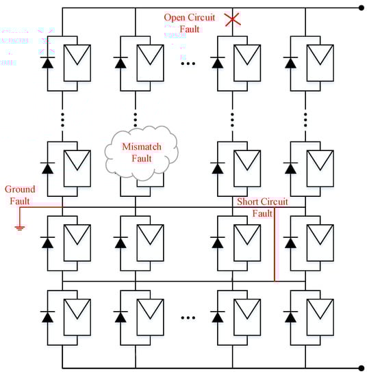
Figure 1.
Four types of faults in a photovoltaic (PV) system.
Different types of faults impact a PV system in different aspects (e.g., variation of voltage or current), and hence produce different I-V characterization curves []. Figure 2 shows the curves for several typical types of faults. A short circuit fault will bring a reduced open circuit voltage () compared with the normal curve. The mismatch fault and open circuit fault will present similar morphology with an inflection point (Mathematically, inflection points are the un-derivable points of an I-V curve and a more detailed description is shown in []), but the I-V curve parameters are different for the two types of faults. Hence, the I-V curves can be used in fault detection and verification in our algorithm.
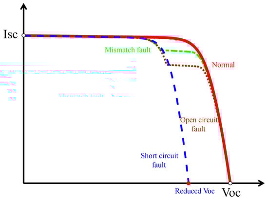
Figure 2.
I-V curves of PV array for different faults.
2.2. Series and Parallel Connections of PV Arrays
In a PV array, PV modules are connected in series, in parallel or their combination to produce the desired current and voltage, shown in Figure 3. The series connection increases the output voltage. A problem is that the deliverable current is dominated by the weakest or fault module in the string, where each module can be viewed as a electricity current source. To reduce such influence, each module is connected in parallel to a diode that can bypass the weak/fault module. The output voltage is the sum of the voltages of the PV modules in the string. A parallel connection can augment the supplied current: the terminal current is the sum of the current of each PV string.
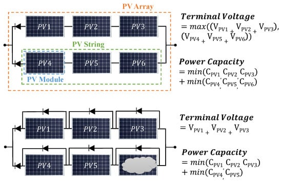
Figure 3.
PV modules connected in series and parallel.
3. System Model
In this section, we present the configuration of our system, which is essentially a switchable PV system with sensors to monitor system working conditions. The system mainly contains three parts: the PV system, the reconfiguration system and the control system.
3.1. Photovoltaic System
PV systems are generally classified by their functional and operational requirements, and the main classifications are grid-connected and stand-alone systems []. PV systems can be designed to provide DC and/or AC power service []. In our work, we augment existing photovoltaic systems structure with fault detection and analysis functionalities. We focus on such PV array faults: short circuit fault, open circuit fault, mismatch fault and power loss fault due to low irradiance. Several typical PV array configurations have been proposed in both industry and academia [,,,]. These configurations have different tolerance for the adverse work environment []. In our work, we use Total Cross-Tied (TCT) configuration in which PV modules are firstly connected in parallel into a “group” and groups are connected in series. The TCT configuration has better tolerance to the working environment.
3.2. Reconfiguration System
In our work, we use a switching matrix component to enable automatic PV system fault detection, shown in Figure 4. There are different reconfiguration models available []. The six-switches model employs six switched for each PV module to enable a fully flexible configuration []. The three-switches model allows system designers to define connection methods (in series or parallel) only for adjacent modules, which is less flexible yet cost effective compared to the six-switches model [,]. In our work, we use the three-switches model that is stable, low-cost, easy to implement and satisfies the control requirements for reconfiguration of a TCT PV array.
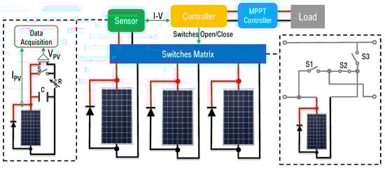
Figure 4.
Architecture of PV system.
3.3. Control System
The control system is a center part of the whole system. It reads in the I-V curves produced by the PV module sensors and conducts fault analysis by controlling the reconfiguration process. There is existing commercial equipment [] to trace the I-V curves of a PV array/sub-array.
The control component is the most important part that controls the whole system signals to implement reconfiguration and analyze the I-V curves of PV arrays and classify the types of faults. The whole system model shown in Figure 4. The controller as the main coordination component connects with a PV array and sensor. By means of a sensor that is designed to be implemented in commercial equipment [] and changing the topology of switches, we can acquire different parts of the I-V curve.
4. Diagnostic Methodology
PV systems are vulnerable to faults, which not only decrease the efficiency of PV systems but also lead to serious consequences (e.g., property loss and human life threat). In order to prevent a dangerous situation, it is critical to locate and classify the faults as soon as possible. In this work, we introduce a new method that applies I-V curve analysis and dynamic reconfiguration to detect and analyze different types of faults. We first present the overall fault detection process and then explain in detail how each type of fault is detected.
4.1. The Fault Detected Process
We aim at figuring out whether there exists a fault, the number and the type of faults. If power loss percentage exceeds a threshold, a diagnostic process is started. In a diagnostic process, the controller should acquire the I-V curve of the whole array, scan the curve to find if there is an inflection point, and compare the value of short current and open voltage with the ideal condition, in order to find out whether faults exist. Here, we denote the voltage of inflection point by , and the corresponding current of this inflection point is . Both parameters can be obtained by analyzing the tangent slope transformation.
If faults are found in the PV system, our reconfiguration system will perform corresponding actions to locate the faults. We adopt series-parallel configurations in this paper. Based on this, we introduced a dichotomy-based method to locate faults. The proposed method will perform efficiently by pruning the branches during segmentation iterations, considering the fact that, in most cases, the number of faults is small or the faults are densely distributed. The method is shown in Algorithm 1.
| Algorithm 1 Fault Detected |
| Input: the whole as argument passed to function, M is the number of groups of this array |
| Output: array with only one type of fault |
| 1: function DIVIDE() |
| 2: |
| 3: if then |
| 4: |
| 5: |
| 6: else if then |
| 7: |
| 8: else |
| 9: |
| 10: end if |
| 11: while do |
| 12: |
| 13: |
| 14: DIVIDE() recursive call the function |
| 15: |
| 16: DIVIDE() recursive call the function |
| 17: end while |
| 18: |
| 19: return |
| 20: end function |
Firstly, the input of Algorithm 1 is the I-V curve for the whole array. The function aims to find a subarray with only one type of fault, and variable is introduced to find the number of fault types. If the value of at the end of the calculation is larger than 1, the whole array is divided into a two part process that is conducted for each part. The recursive function continues until, for each part, only one type of fault exists. For each with a single type of fault, Algorithm 2 (explained later) is invoked to find out the exact fault.
4.2. I-V Curve Analysis Process
With the proposed I-V curve analysis, the location of fault and the identification of the fault type is achieved, the whole process of which is illustrated in Figure 5 and formally defined by Algorithm 2. Curve analysis is based on pattern recognition. The following sub-sections give the details on the recognition of different types of faults.
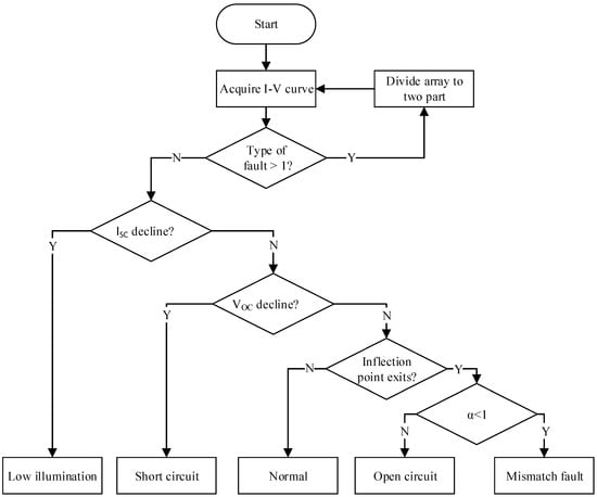
Figure 5.
The flowchart of the I-V curve diagnostic process.
4.2.1. Analysis of Open Circuit Faults
We assume that the group has some failures of the same fault type, for example, n modules with open circuit fault. For groups under normal operating conditions, the short-circuit current of each group is , and the short-circuit current of the failure group is:
If a module has an open circuit fault inside, the bypass diode will be activated, which reduces the overall current of the group to which the fault module belongs. The current decrease will suppress the current flowing into other serially connected groups. Hence, the I-V curve will show an inflection point. To distinguish open circuit faults from mismatched faults that have similar curve shapes, the corresponding current and voltage value of the inflection point should be precisely computed. The computation is given as follows:
In the above equations, n is the number of fault modules in a group, N is the number of modules in a group and M is the number of groups, is the number of groups that have open circuit faults, and is the reverse bias voltage of the bypass diode.
4.2.2. Analysis of Mismatch Faults
Mismatch faults are caused by the interconnection of solar cells or modules which do not have identical properties or which experience different conditions from one another. We assume that, in the group, n modules have mismatch losses. For groups under normal operating conditions, the short-circuit current of each group is , and the short-circuit current of the failure group is:
To distinguish mismatch faults from open circuit faults, we find that the short-circuit current of the fault module is larger than 0 for the mismatch fault case (note that the value of the current depends on the load). Thus, we introduce a parameter with a value range to model this difference. The computation of the inflection point for a mismatch fault is given below:
In the above equations, n is the number of fault modules in a group, is the number of groups with mismatch faults that cause the bypass diode to be turned on, and is the reverse bias voltage of the bypass diode.
4.2.3. Analysis of Short Circuit Faults
For TCT configuration, once a short circuit fault occurs inside a group, this group would be totally short circuited, the voltage would drop to zero, and the current will flow through the short circuit branch. Thus, a circuit fault has a significant impact on the open circuit voltage of the array but has little effect on current. We assume that m groups have failures in the array, the current of the array can be described as: , and the open circuit voltage can be written as Equation (7):
where is the operating current of group, is the open circuit voltage of group, and m is the number of fault groups in array.
Algorithm 2 gives the algorithm to detect faults by computing short circuit current , open circuit voltage , and the voltage of inflection point in the I-V curve. Since the open-circuits and mismatch faults have similar patterns, we introduce a parameter to distinguish the two cases. is defined by Equation (8):
where is the current of inflection point, is the short circuit current of one PV module, and is the short circuit current acquired in the I-V curve.
| Algorithm 2 IV Curve |
| Input: from Algorithm 1 |
| Output: type of fault |
| 1: M |
| 2: if then more than one group |
| 3: if then |
| 4: . |
| 5: else if then |
| 6: . |
| 7: else if then |
| 8: if then |
| 9: . |
| 10: else |
| 11: . |
| 12: end if |
| 13: else |
| 14: end if |
| 15: else only one group |
| 16: if then |
| 17: . |
| 18: else |
| 19: . |
| 20: end if |
| 21: end if |
Algorithm 2 applies the principles introduced in Section 4.2.1, Section 4.2.2 and Section 4.2.3 and finally gives the results of fault type in a sub-array. For each part with only one type of fault, in Algorithm 3, a dichotomy-based process is conducted until the fault is located in a sub-array that satisfies user requirements on analysis precision.
| Algorithm 3 Location |
| Input: from Algorithm 1 |
| Output: with only one group |
| 1: |
| 2: while do |
| 3: |
| 4: |
| 5: if then part2 without fault, part1 is the finally target subarray |
| 6: |
| 7: else |
| 8: |
| 9: end if |
| 10: end while while loop could locate the fault in a group |
| 11: return |
In a dichotomy-based process, if the I-V curve for one part of the divided array is normal, then fault locating will not be further conducted to this array, thus reducing analysis efforts. If needed, by dividing the array into two parts through the dichotomy algorithm continuously, we would be able to locate the group of fault finally. Based on this idea, the same copy to column faults can proceed, and our method is capable of locating a fault existing on a single PV module.
5. Case Study
5.1. Simulation Platform
To validate the proposed method, we develop a system with a PV array, switch matrix circuit, controller and variable DC source with sensors using Matlab/Simulink (Matlab R2016b, MathWorks, Natick, MA, USA) (shown in Figure 6). To ensure accurate simulation of PV modules, we adopt the classical single diode model derived from physical principles []. The specification of each PV module comes from the System Advisor Model (SAM) (which is developed by the National Renewable Energy Laboratory (NREL) with funds from the U.S. Department of Energy) libraries and Databases website []. Temperature and irradiance values have been entered as input data into the module. The controller is implemented as a Matlab function block based on Algorithms 1–3. Programmable switches are used in the switch matrix circuit. This system allows us to conduct experiments on fault detection, classification and location. is
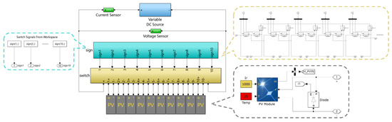
Figure 6.
Architecture of the simulation platform.
5.2. Simulation Results and Analysis
In order to demonstrate the effectiveness of the proposed method, we build a PV array in the simulation. The PV module specifications are: V, A, V, A; temperature coefficient of is C and is C. Each PV module is connected with a bypass diode in parallel, and the configuration of the PV array is TCT configuration.
We randomly generated four different faults of three types located in different modules of the PV array. Partial shadow is used as an example in the case study to cause a mismatch fault. We use to indicate the coordinate (row and column) of the fault location, as shown in Table 1.

Table 1.
Simulated faults and coordinates.
The detailed analysis procedure of the algorithm is shown in Figure 7. For each analyzed array/sub-array, the fault modules are illustrated with dark blocks in the array, and the corresponding I-V curve is also given. By the algorithm, the array can be divided into two sub-arrays, and the corresponding I-V curve of each sub-array is portrayed below the sub-array structure. We can see that the two I-V curves are not normal, i.e., there exist some faults in both sub-arrays. By executing the algorithm iteratively, we can find all fault types and their corresponding locations.
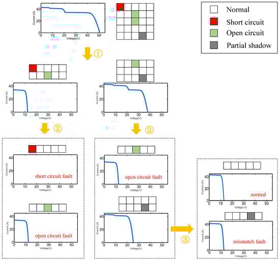
Figure 7.
Analysis procedure of the implemented algorithm.
6. Discussion
In this section, we discuss the analysis performance, analysis overhead, power consumption and cost of the proposed method.
Analysis performance. The analysis performance is decided by how deep the segmentation process goes. First, user requirements on detection precision affects the depth of the segmentation. Second, the distribution of faults is also a deciding factor. Taking a PV array with N panels, for example, the worst-case number of detection is . However, if the number of faults is small or the faults are densely distributed, the method will perform efficiently by pruning the branches (with no fault panels) during the segmentation iterations.
Analysis overhead. Fault detection time overhead is mainly related to the process of obtaining the I-V curve. The time for one test by an I-V tracer is very small, for example, the Solmetric PVA-600 tracer [] can obtain an I-V curve within 240 ms. Taking a panel array for example, the computation time is about 10 ms given that the algorithms run on a STM32F030F4P6 [] micro-controller (STMicroelectronics, Geneva, Switzerland). The reconfiguration time is within 50 ns for a BUK7Y10-30B Metal-Oxide-Semiconductor Field-Effect Transistor(MOSFET)-based switch system (Nexperia, Nijmegen, The Netherlands) []. Thus, the total analysis time is , in the worst case.
Power consumption. Additional power consumption mainly comes from two aspects. The first is the switch matrix, and the array needs transistors. For each BUK7Y10-30B transistor, the power consumption is about W. In the worst-case, only of the transistors are on. Then, the power consumption of the matrix is W. The second aspect is the control system. A typical power consumption of an embedded control system is about 50 W. Using the PV modules in the case study, the power output (without faults) in standard working conditions (C) is . Therefore, the power overhead ration is .
Cost analysis. The PV array costs RMB 25,000, and the cost of the automatic fault detection system is RMB , the details of which are given by Table 2. Therefore, the cost overhead is 313.5/25,000 = 1.25%.
Table 2.
Cost analysis of the proposed method.
The CPLD is the abbreviation for Complex Programmable Logic Device; The PCB is the abbreviation for Printed circuit board; RCL represents resistor(R), capacitor(C), and inductor(L).
7. Conclusions
Fault detection is indispensable for ensuring that PV systems run in a safe, reliable, and available status. Automatic fault detection and classification remains a major challenge. In this paper, a fault analysis method is proposed, which not only detects and locates PV faults but also classifies the faults based on their distinguishable patterns in I-V curves.The main contribution of this paper is automatic fault detection and location compared to traditional laborious manual methods.The method can be applied in both small-scale and large-scale PV systems. We have evaluated the proposed method by a Matlab simulation system. Experimental results demonstrate that the method can precisely locate PV faults and classify fault types. In the future, we plan to build a hardware prototype to evaluate the effectiveness of the method in real-life systems and further optimize the method.
Acknowledgments
This article was partially supported by National Natural Science Foundation of China (61532007, 61672140), Collaborative Innovation Center of Major Machine Manufacturing in Liaoning, and State Key Laboratory of Synthetical Automation for Process Industries (PAL-N201503).
Author Contributions
Dong Ji, Cai Zhang, Nan Guan conceived the work; Dong Ji, Cai Zhang and Ye Ma performed the simulations; Dong Ji and Cai Zhang wrote the manuscript; Mingsong Lv, Nan Guan supervised the work and provided critical review.
Conflicts of Interest
The authors declare no conflict of interest.
References
- Van der Hoeven, M. Technology Roadmap-Solar Photovoltaic Energy; International Energy Agency: Köln, Germany, 2014. [Google Scholar]
- Köntges, M.; Kurtz, S.; Jahn, U.; Berger, K.; Kato, K.; Friesen, T.; Van Iseghem, M. Review of Failures of Photovoltaic Modules. In International Energy Agency (IEA) PVPS Task 13; IEA: Köln, Germany, 2014. [Google Scholar]
- Cooper Bussmann Inc. Complete and Reliable Solar Circuit Protection. Eaton, 2014. Available online: http://www.eaton.fr/ecm/groups/public/@pub/@electrical/documents/content/10191.pdf (accessed on 9 May 2017).
- Togami Electric Mfg.Co.,Ltd. (Saga, Japan). Photovoltaic Module Fault Detectors. June 2014. Available online: https://www.togami-elec.co.jp/english/pdf/pv.pdf (accessed on 9 May 2017).
- Asea Brown Boveri Ltd. (Zurich, Switzerland). Symphony Plus for Solar Integrated Automation and Services for Photovoltaic Plants. 2015. Available online: https://library.e.abb.com/public/5963de567cb74e4282e5ecce1ece6363/2VAA005055_PV_Automation%20and%20Service_Brochure_2015.pdf (accessed on 9 May 2017).
- Chouder, A.; Silvestre, S. Automatic supervision and fault detection of PV systems based on power losses analysis. Energy Convers. Manag. 2010, 51, 1929–1937. [Google Scholar] [CrossRef]
- Silvestrea, S.; Chouderb, A.; Karatepec, E. Automatic fault detection in grid connected PV systems. Sol. Energy 2013, 94, 119–127. [Google Scholar] [CrossRef]
- Firth, S.K.; Lomas, K.J.; Rees, S.J. A simple model of PV system performance and its use in fault detection. Sol. Energy 2010, 84, 624–635. [Google Scholar] [CrossRef]
- Alonso-Garcia, M.C.; Ruiz, J.M.; Chenlo, F. Experimental study of mismatch and shading effects in the I–V characteristic of a photovoltaic module. Sol. Energy Mater. Sol. Cells 2006, 90, 329–340. [Google Scholar] [CrossRef]
- Lin, X.; Wang, Y.; Zhu, D.; Chang, N.; Pedram, M. Online Fault Detection and Tolerance for Photovoltaic Energy Harvesting Systems. In Proceedings of the International Conference on Computer-Aided Design, San Jose, CA, USA, 5–8 November 2012; pp. 1–6. [Google Scholar]
- Serna-Garcés, S.I.; Bastidas-Rodríguez, J.D.; Ramos-Paja, C.A. Reconfiguration of Urban Photovoltaic Arrays Using Commercial Devices. Energies 2016, 9, 2. [Google Scholar] [CrossRef]
- Balato, M.; Costanzo, L.; Vitelli, M. Series-Parallel PV array re-configuration: Maximization of the extraction of energy and much more. Appl. Energy 2015, 159, 145–160. [Google Scholar] [CrossRef]
- Balato, M.; Costanzo, L.; Vitelli, M. Reconfiguration of PV modules: A tool to get the best compromise between maximization of the extracted power and minimization of localized heating phenomena. Sol. Energy 2016, 138, 105–118. [Google Scholar] [CrossRef]
- Zhao, Y. Fault detection, classification and protection in solar photovoltaic arrays. In Dissertations & Theses, Gradworks; Northeastern University: Boston, MA, USA, 2016. [Google Scholar]
- Drews, A.; Keizer, A.C.D.; Beyer, H.G.; Lorenz, E.; Betcke, J.; Van Sark, W.G.J.H.M.; Heydenreichd, W.; Wiemkend, E.; Stettlere, S.; et al. Monitoring and remote failure detection of grid-connected PV systems based on satellite observations. Sol. Energy 2007, 81, 548–564. [Google Scholar] [CrossRef]
- Guide To Interpreting I-V Curve Measurements of PV Arrays. Available online: http://resources.solmetric.com/get/Guide%20to%20Interpreting%20I-V%20Curves.pdf (accessed on 9 May 2017).
- Petrone, G.; Ramos-Paja, C.A. Modeling of photovoltaic fields in mismatched conditions for energy yield evaluations. Electr. Power Syst. Res. 2011, 81, 1003–1013. [Google Scholar] [CrossRef]
- Kaundinya, D.P.; Balachandra, P.; Ravindranath, N.H. Grid-connected versus stand-alone energy systems for decentralized power-A review of literature. Renew. Sustain. Energy Rev. 2009, 13, 2041–2050. [Google Scholar] [CrossRef]
- Almahjoub, A.A.; Ailane, A.; Rachik, M.; Essadki, A.; Bouyaghroumni, J. Non-linear Control of a Multi-loop DC-AC Power Converter Using in Photovoltaic System Connected to the Grid. Int. J. Electr. Comput. Sci. 2012, 12, 10–16. [Google Scholar]
- Kaushika, N.D.; Gautam, N.K. Energy yield simulations of interconnected solar PV arrays. IEEE Trans. Energy Convers. 2003, 18, 127–134. [Google Scholar] [CrossRef]
- Giraud, F.; Salameh, Z. Analysis of the effects of a passing cloud on a grid-interactive photovoltaic system with battery storage using neural networks. IEEE Trans. Energy Convers. 1999, 14, 1572–1577. [Google Scholar] [CrossRef]
- Wang, Y.J.; Hsu, P.C. An investigation on partial shading of PV modules with different connection configurations of PV cells. Energy 2011, 36, 3069–3078. [Google Scholar] [CrossRef]
- Ramaprabha, R.; Mathur, B.L. A comprehensive review and analysis of solar photovoltaic array configurations under partial shaded conditions. Int. J. Photoenergy 2012, 2012, 120214. [Google Scholar] [CrossRef]
- Belhachat, F.; Larbes, C. Modeling, analysis and comparison of solar photovoltaic array configurations under partial shading conditions. Sol. Energy 2015, 120, 399–418. [Google Scholar] [CrossRef]
- Alahmad, M.; Chaaban, M.A.; kit Lau, S.; Shi, J.; Neal, J. An adaptive utility interactive photovoltaic system based on a flexible switch matrix to optimize performance in real-time. Sol. Energy 2012, 86, 951–963. [Google Scholar] [CrossRef]
- Kim, H.; Shin, K.G. On dynamic reconfiguration of a large-scale battery system. Proceedings of 15th IEEE Real-Time and Embedded Technology and Applications Symposium, San Francisco, CA, USA, 13–16 April 2009; pp. 87–96. [Google Scholar]
- He, L.; Kim, E.; Shin, K.G. Resting weak cells to improve battery pack’s capacity delivery via reconfiguration. In Proceedings of the Seventh International Conference on Future Energy Systems, New York, NY, USA, 21–24 June 2016. [Google Scholar]
- Nguyen, D.; Lehman, B. An Adaptive Solar Photovoltaic Array Using Model-Based Reconfiguration Algorithm. IEEE Trans. Ind. Electron. 2008, 55, 2644–2654. [Google Scholar] [CrossRef]
- Hernday, P. Field Applications of I-V Curve Tracers in the Solar PV Industry. Proceedings of IEEE Silicon Valley Photovoltaics Society (SVPVS) Meeting, Santa Clara, CA, USA, 14 November 2012. [Google Scholar]
- Luque, A.; Hegedus, A.; Gray, J.L. The Physics of the Solar Cell. In Handbook of Photovoltaic Science and Engineering; John Wiley and Sons: New York, NY, USA, 2010; ISBN 978-0-470-72169-8. [Google Scholar]
- NREL System Advisor Model. Libraries and Databases. Available online: https://sam.nrel.gov/libraries (accessed on 9 May 2017).
- Solemtric. Solmetric PV Analyzer I-V Curve Tracer with SolSensor™ PVA-1000S, PVA-600+ User’s Guide. Available online: http://www.solmetric.net/get/PVA-SolSensor-Users-Guide-Feb19-2014.pdf (accessed on 9 May 2017).
- STMicroelectronics. STM32F030F4P6 Data Sheet. Available online: http://www.mouser.com/ds/2/389/stm32f030f4-956260.pdf (accessed on 9 May 2017).
- Nexperia. BUK7Y10-30B Data Sheet. Available online: http://assets.nexperia.com/documents/data-sheet/BUK7Y10-30B.pdf (accessed on 9 May 2017).
© 2017 by the authors. Licensee MDPI, Basel, Switzerland. This article is an open access article distributed under the terms and conditions of the Creative Commons Attribution (CC BY) license (http://creativecommons.org/licenses/by/4.0/).