
Probabilistic Power Flow Method Considering Continuous and Discrete Variables

Abstract
:1. Introduction
- (1)
- This paper proposes a novel PPF method (CDPF) that can accurately solve PPF problems with continuous and discrete variables simultaneously. In CDPF, multiple probability distributions of continuous variables and discrete variables can be considered together, such as normal distribution (loads), non-normal distribution (WPGs), and binomial distribution (FCGs).
- (2)
- (3)
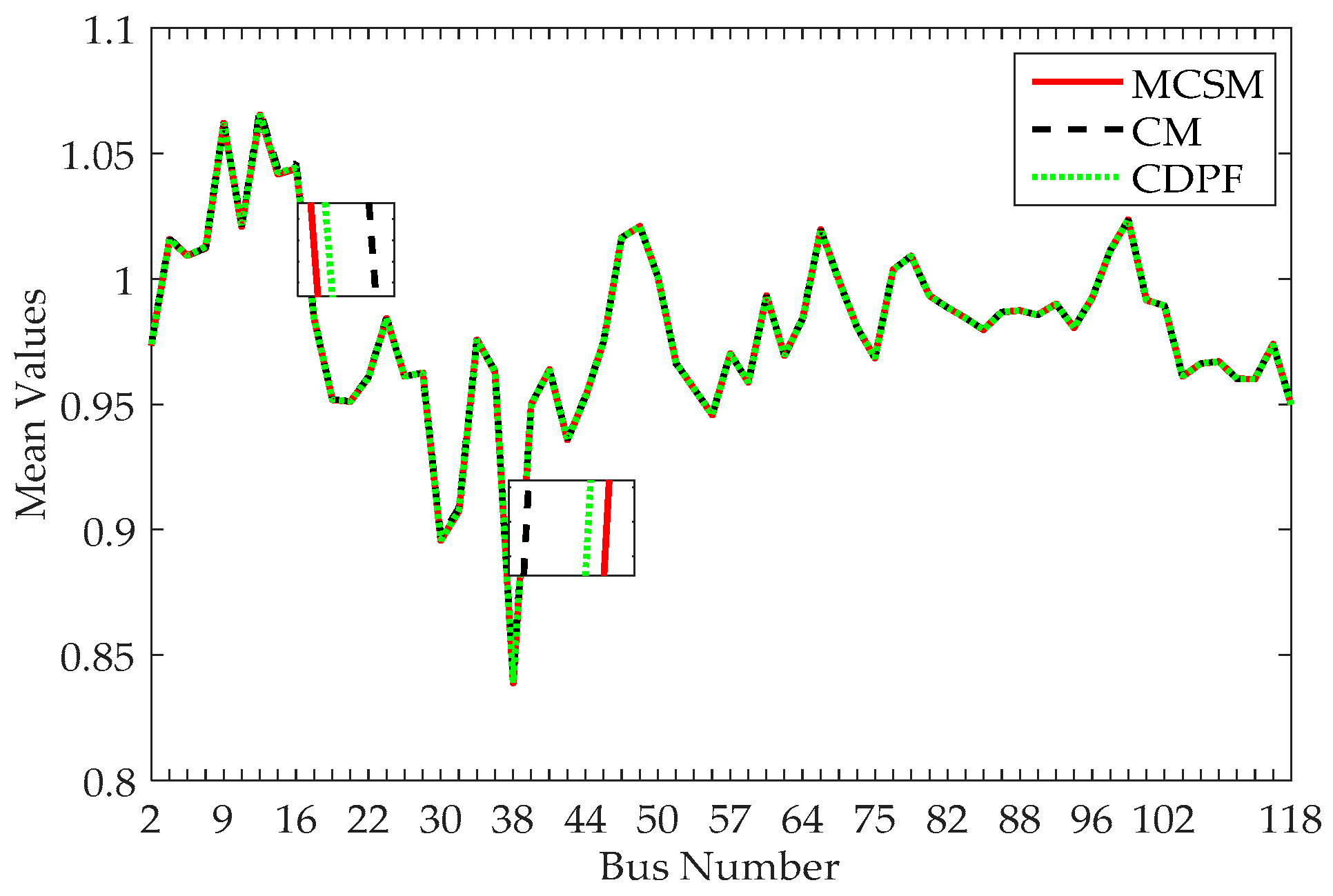
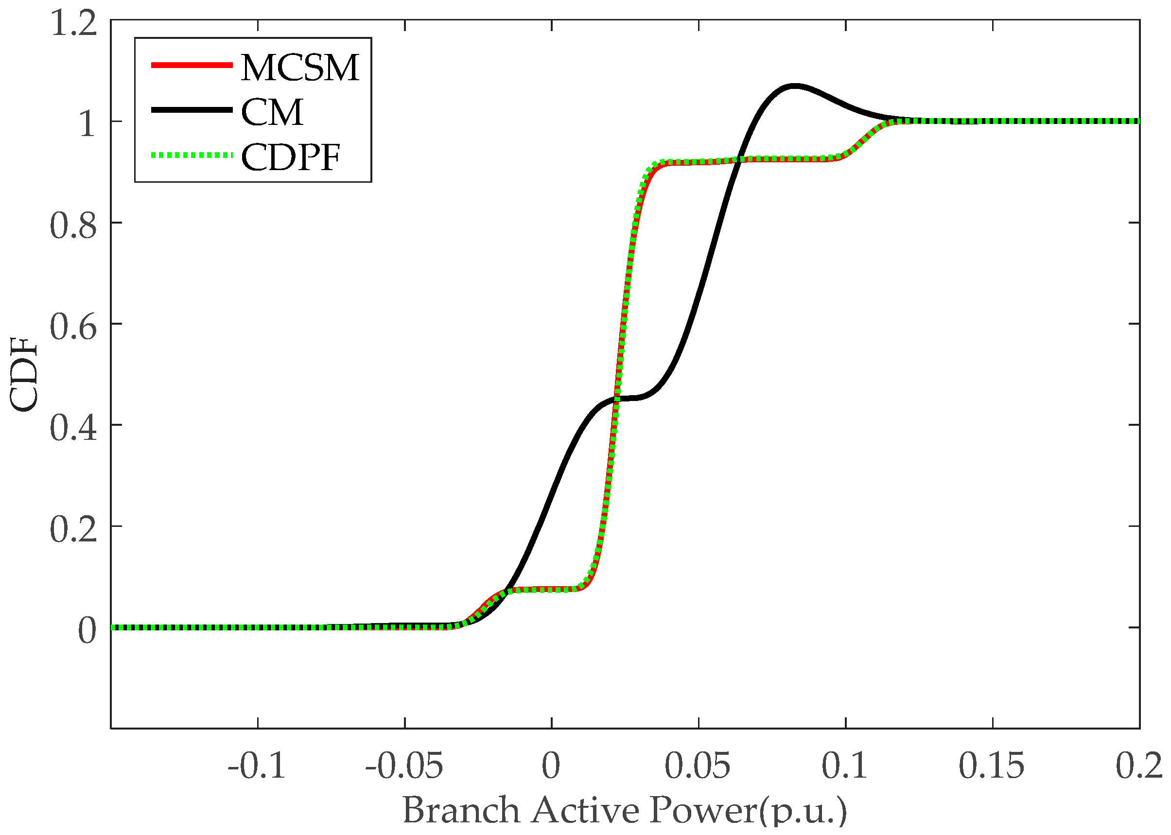
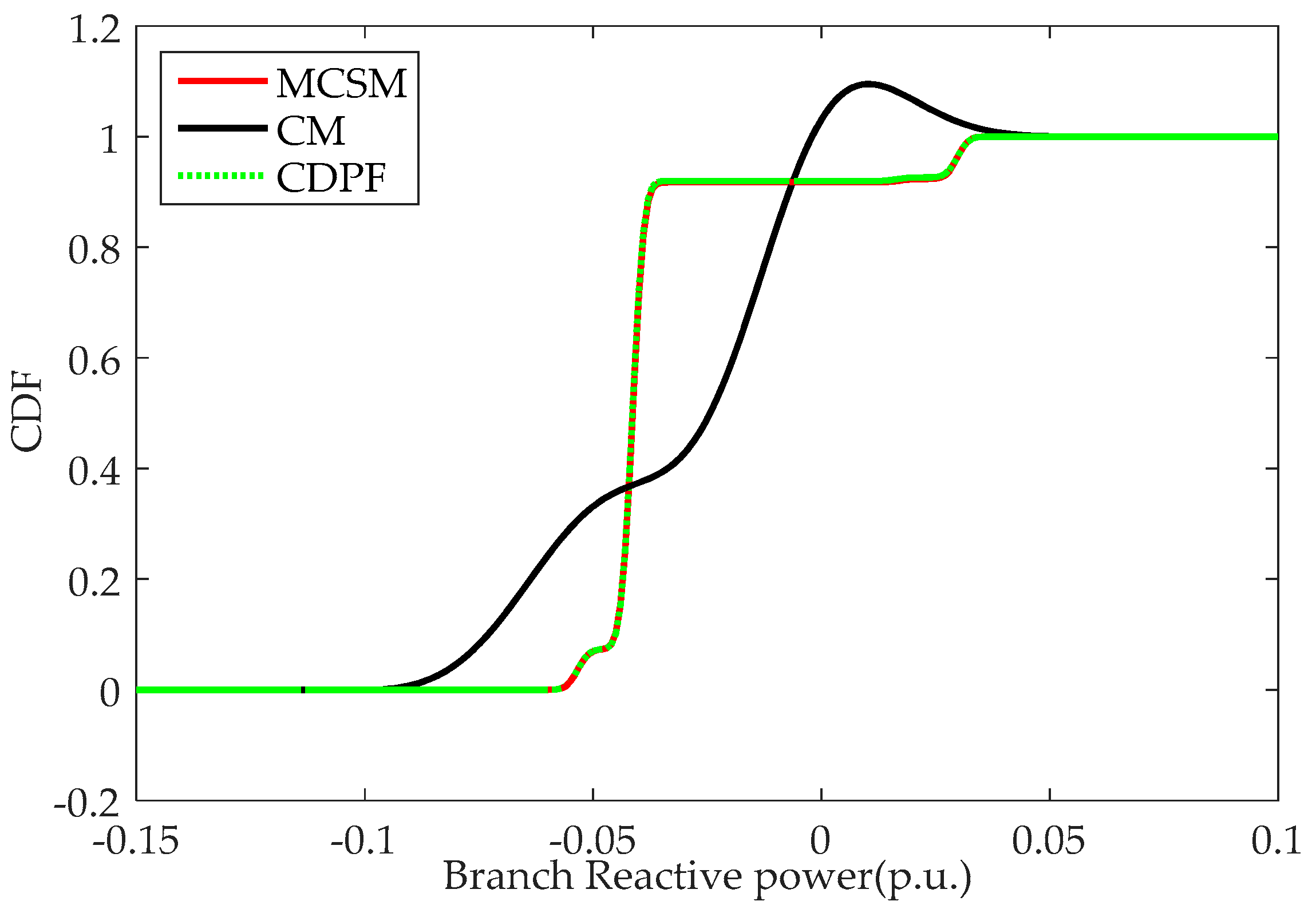
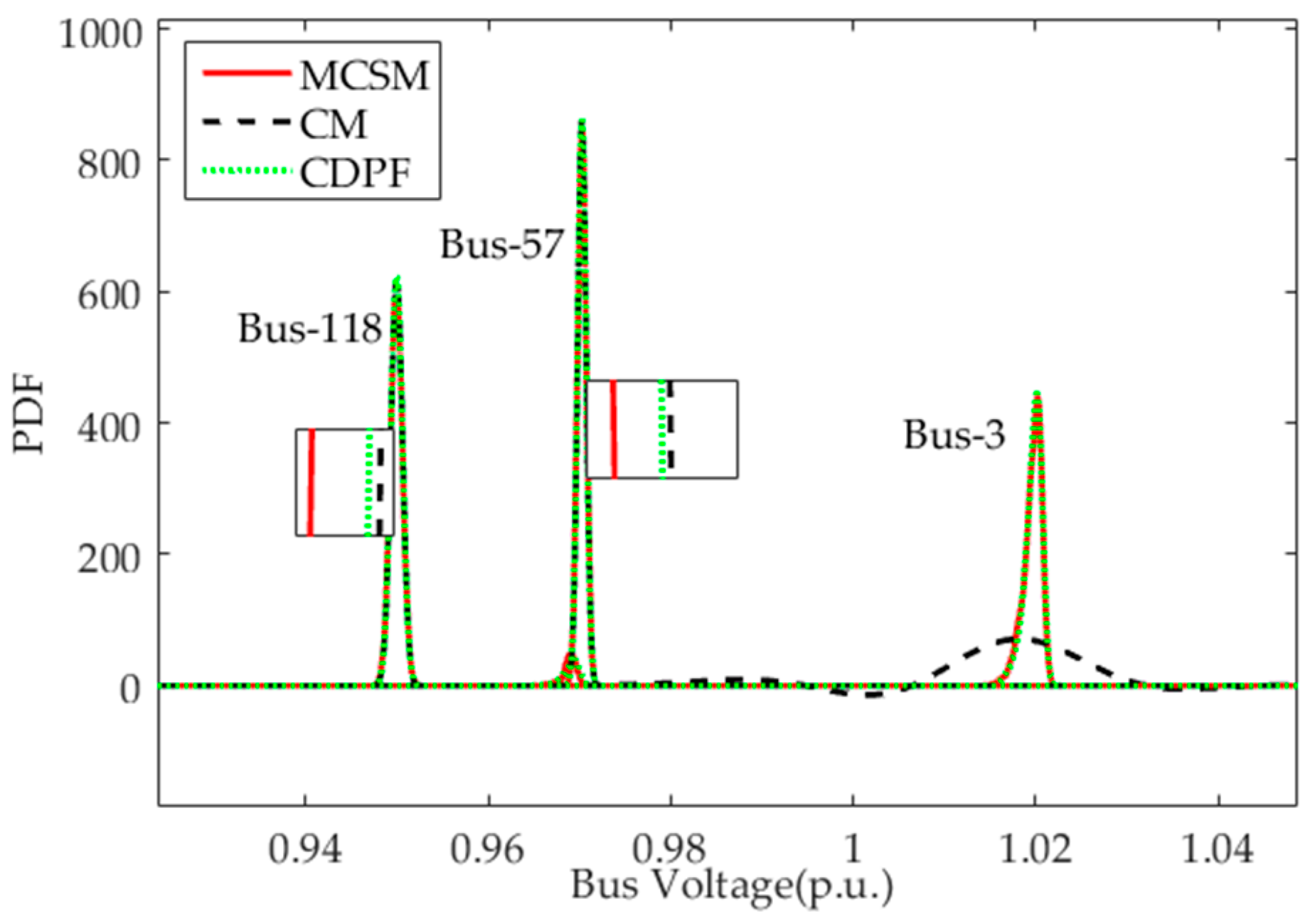
- The accuracy and efficiency of CDPF are verified quite well compared with results of bus voltages and branch power flows obtained by CDPF, CM, and MCSM in IEEE 14-bus and IEEE 118-bus power systems.
2. Probability Distributions of Generations and Loads
2.1. The Output Power PDF of WPGs
2.2. The Active and Reactive Power PDF of Loads
2.3. The Output Power Probability Distribution of FCGs
3. CDPF Method
3.1. Power Flow Responses with Continuous Variables Based on CM
3.1.1. Calculation on Continuous Variable Cumulants
3.1.2. Linear Power Flow Equations
3.1.3. Estimation on Probability Distributions of Power Flow Responses
3.2. Power Flow Responses with Discrete Variables Based on MDPF Calculations
3.2.1. Determination on the Vector of Discrete Variables
3.2.2. Determination on the Active Power and Reactive Power Vector of Generations and Loads
3.2.3. Calculations Based on MDPF
3.3. Convolution of Continuous and Discrete Variables
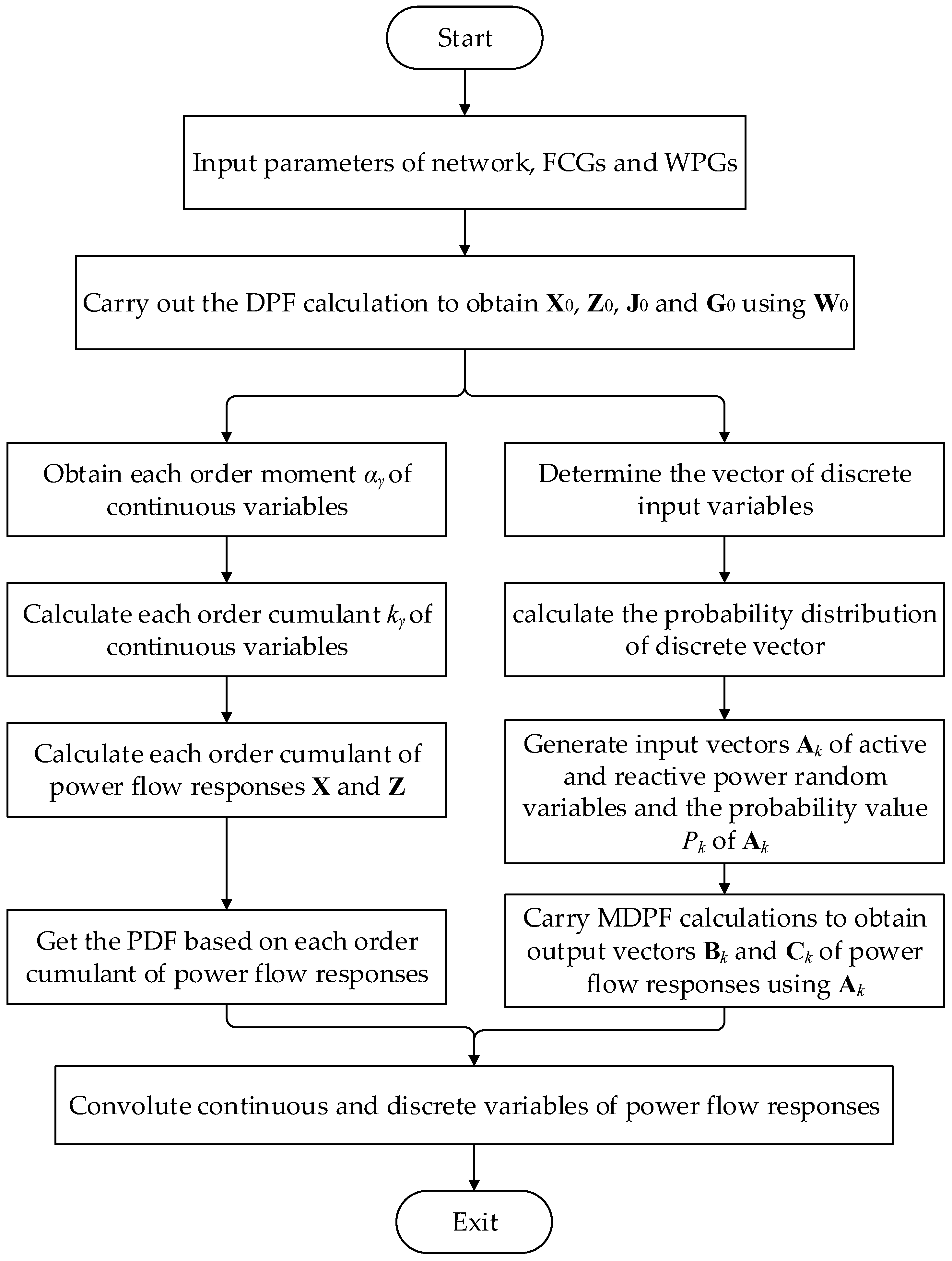
3.4. Implementation Procedure of CDPF
4. Case Studies
4.1. Verification of CDPF by Comparison with MCSM and CM in Accuracy and Efficiency
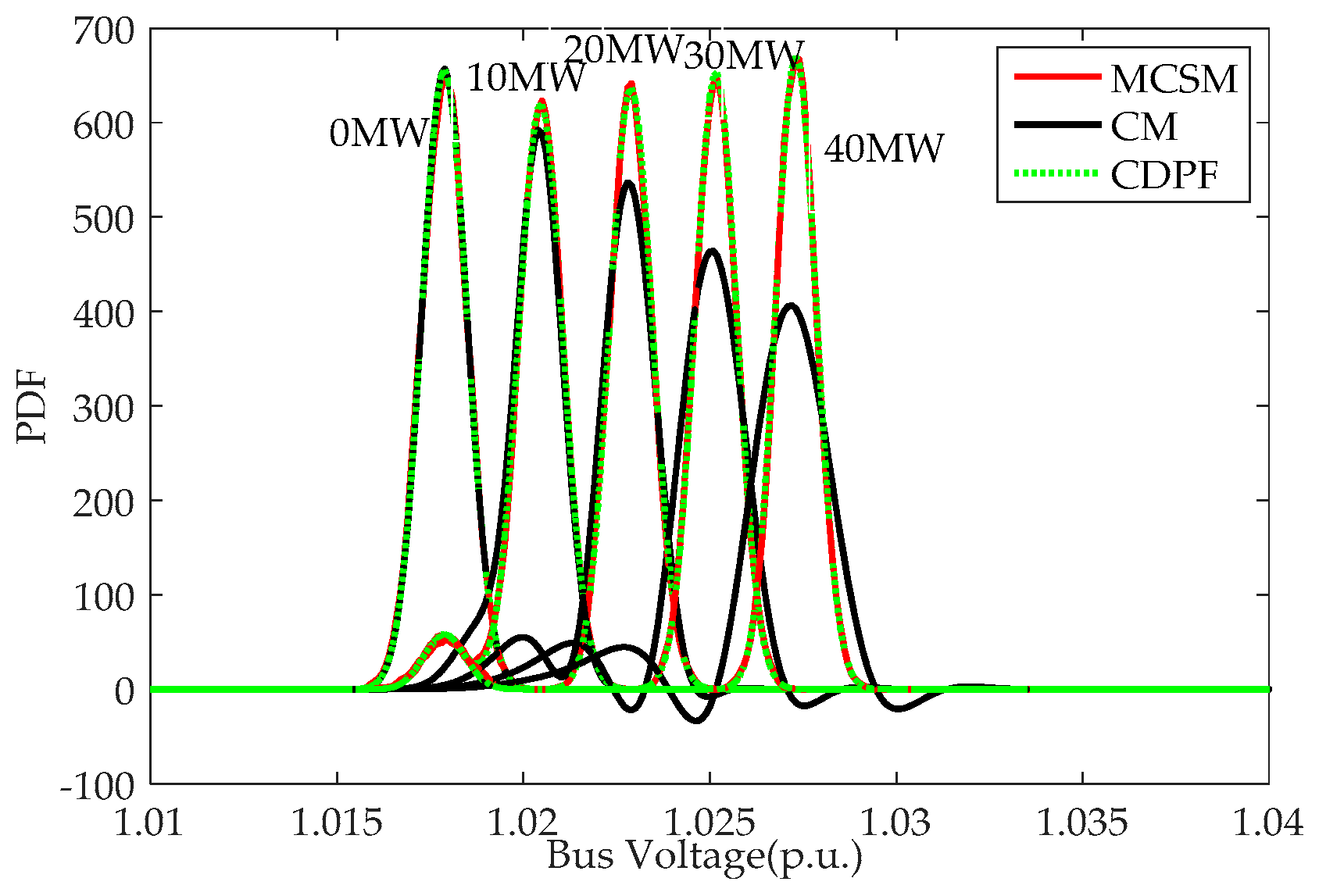
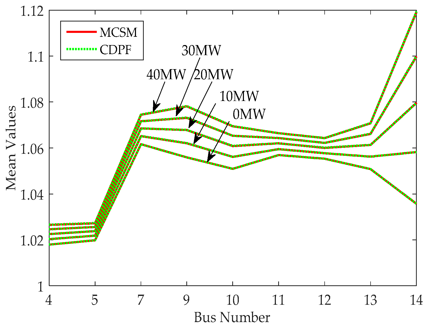
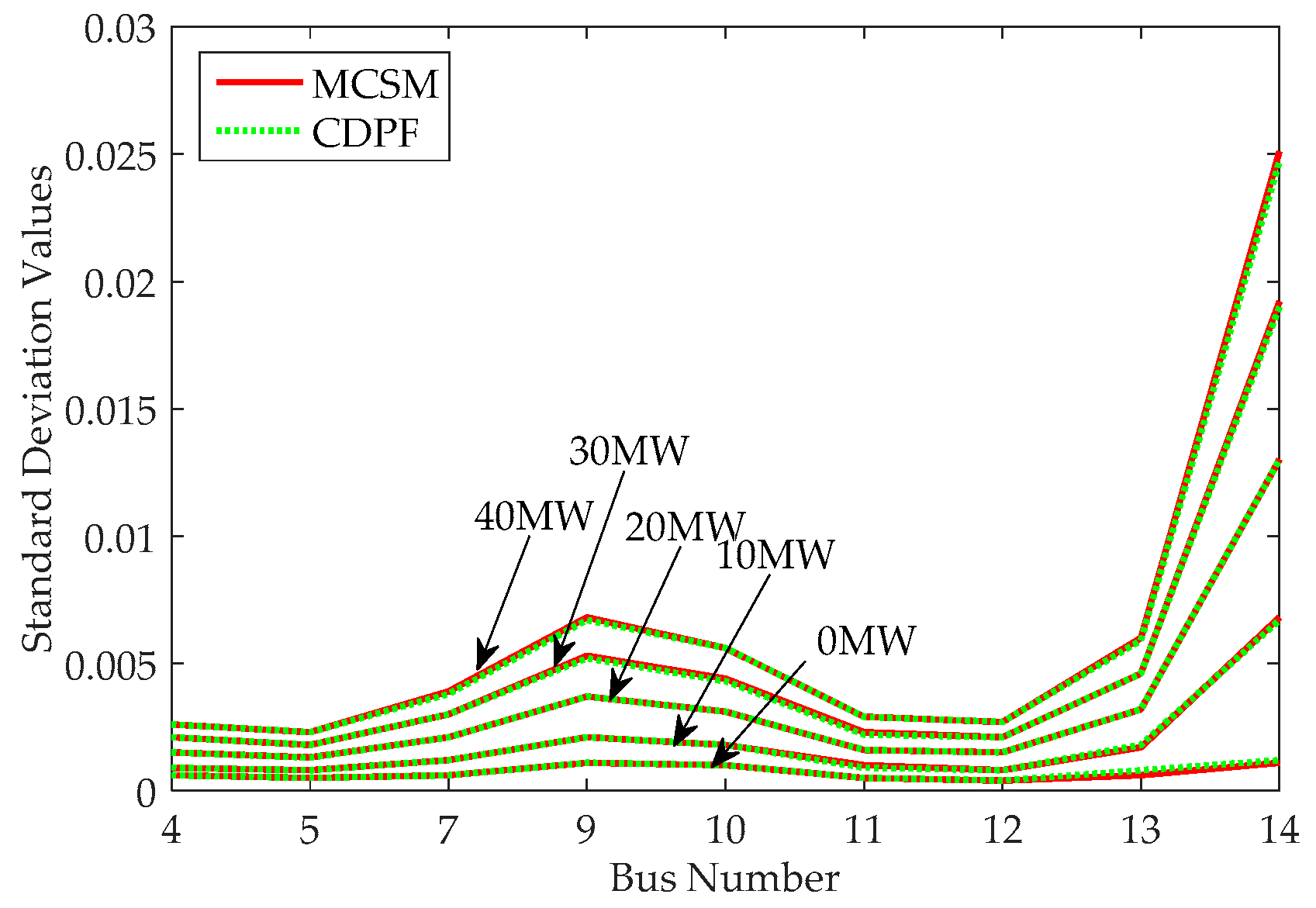
4.2. PPF Analysis on a FCG under Different Rated Powers
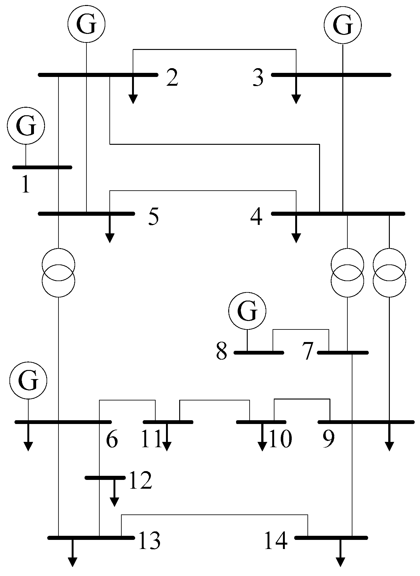
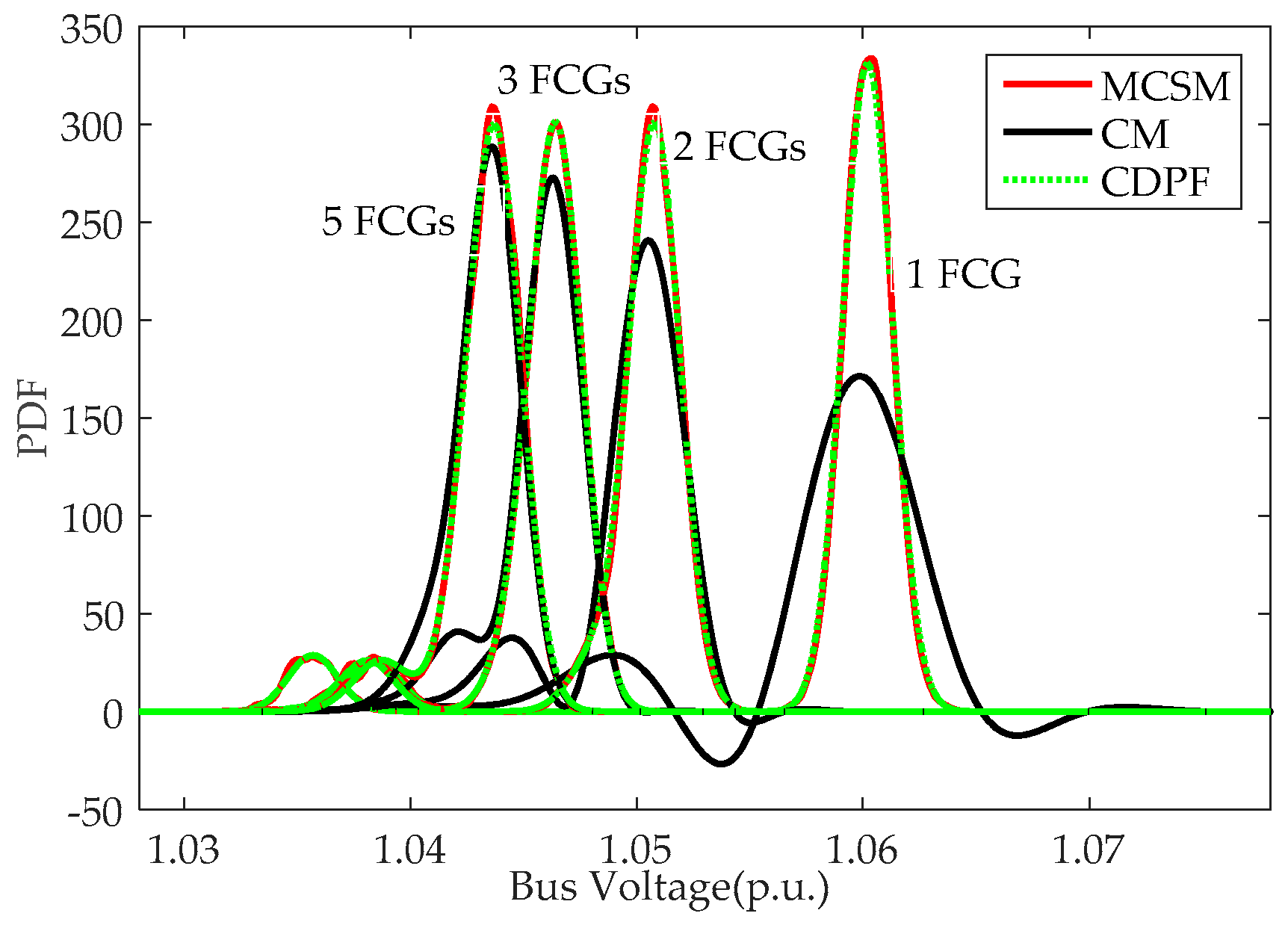
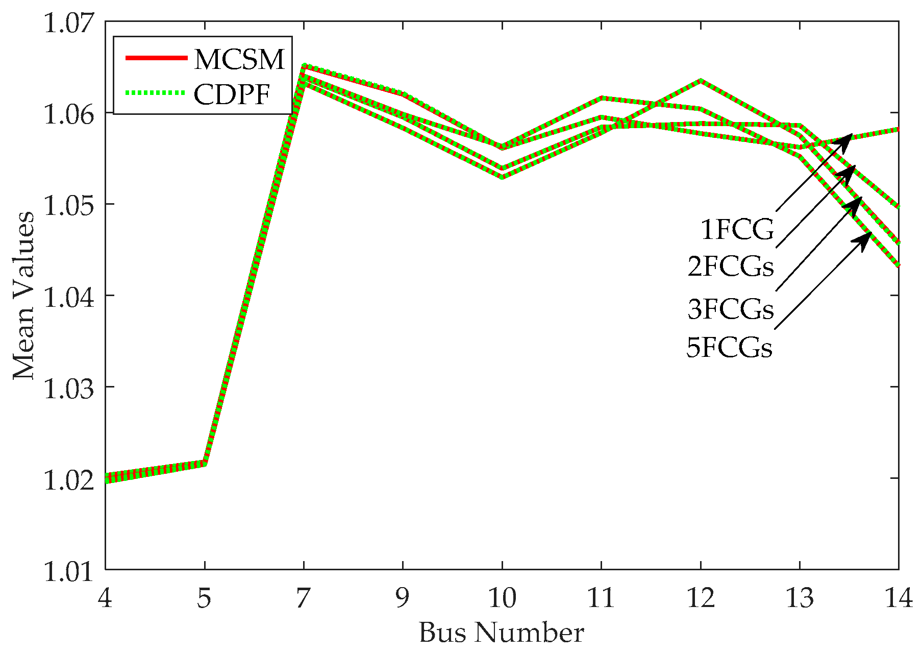
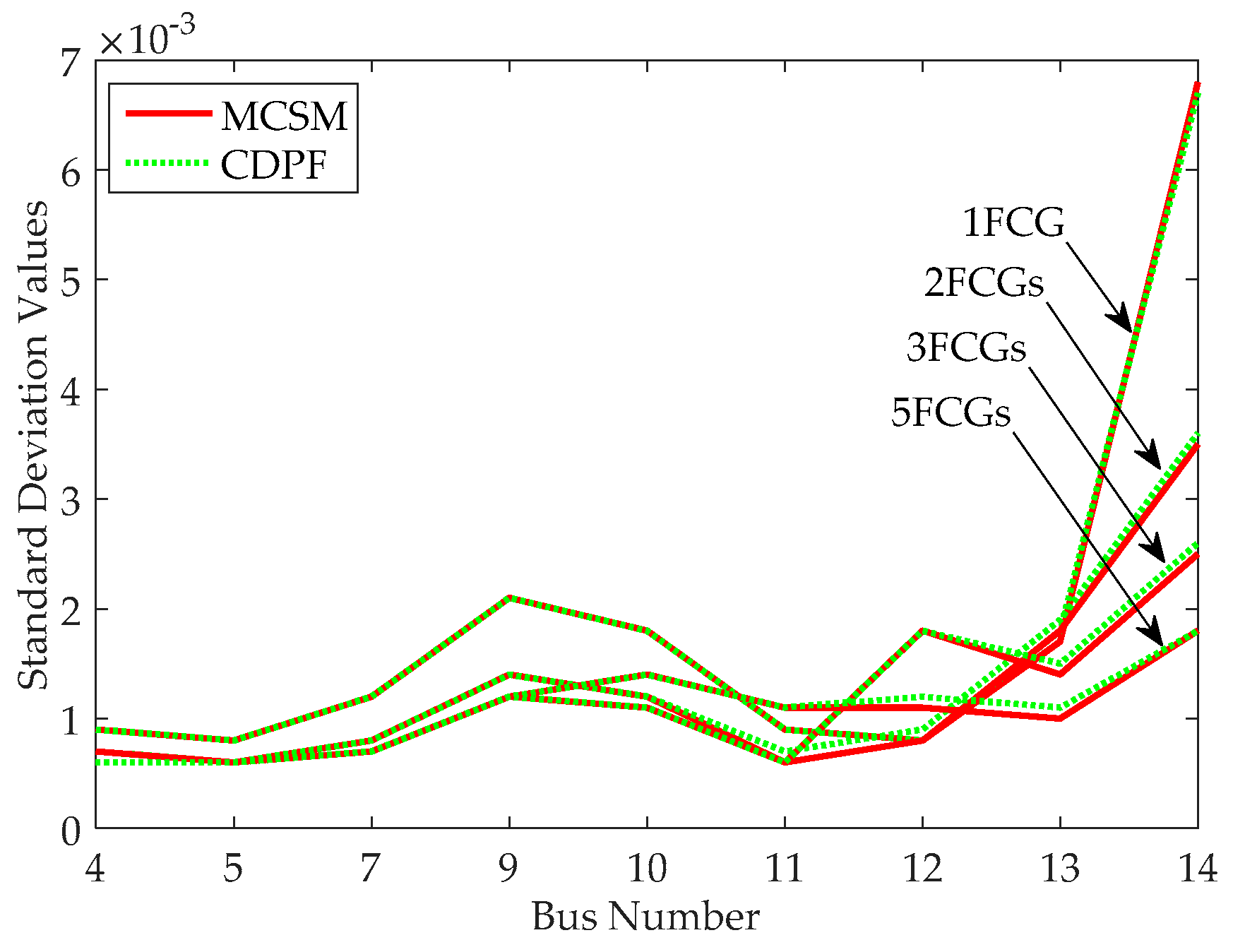
4.3. PPF Analysis on Multiple FCGs in an IEEE 14-Bus Power System
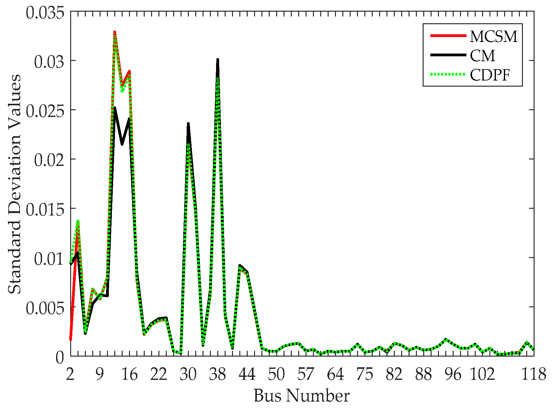
4.4. The Test in the IEEE 118-Bus Power System
5. Conclusions
- (1)
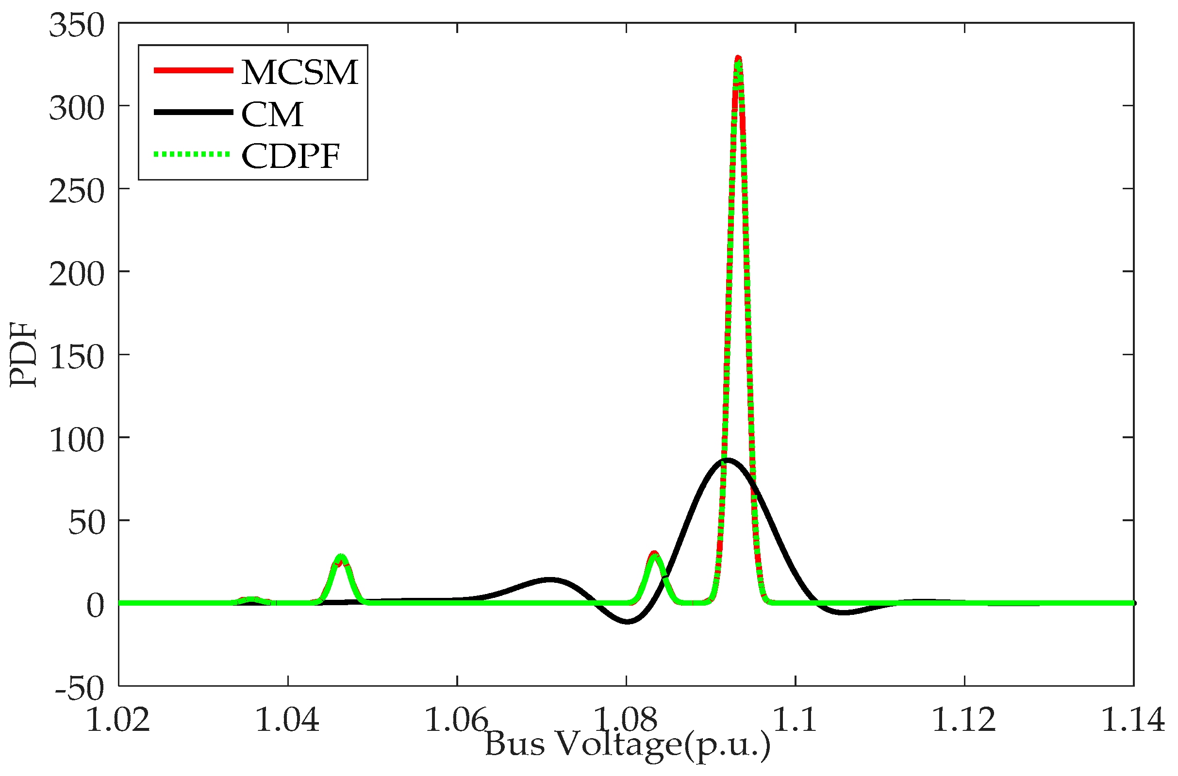
- CDPF has better performance in computation speed compared with MCSM. Additionally, CDPF has a better performance in computation accuracy than CM, especially for the case with the large fluctuation range of input random variables.
- (2)
- CDPF has good performance in the applicability to deal with a discrete variable with different rated powers and multiple discrete variables in power systems.
- (3)
- CDPF has good performance in the applicability to address large power systems with high accuracy and efficiency.
Author Contributions
Conflicts of Interest
Glossary of Acronyms
| PPF | probabilistic power flow |
| CM | cumulant method |
| MCSM | Monte Carlo simulation method |
| CDPF | power flow considering continuous and discrete variables |
| DPF | deterministic power flow |
| MDPF | multiple deterministic power flow |
| probability density function | |
| CDF | cumulative density function |
| GCS | Gram-Charlier series |
| FCG | fuel cell generation |
| WPG | wind power generation |
| CPU | central processing unit |
References
- Borkowska, B. Probabilistic load flow. IEEE Trans. Power Appar. Syst. 1974, 3, 752–759. [Google Scholar] [CrossRef]
- Sun, Y.Y.; Mao, R.; Li, Z.Y.; Tian, W. Constant Jacobian matrix-based stochastic Galerkin method for probabilistic load flow. Energies 2016, 9, 153. [Google Scholar] [CrossRef]
- Chen, Y.; Wen, J.Y.; Cheng, S.J. Probabilistic load flow method based on Nataf transformation and Latin hypercube sampling. IEEE Trans. Sustain. Energy 2013, 4, 294–301. [Google Scholar] [CrossRef]
- Soleimanpour, N.; Mohammadi, M. Probabilistic load flow by using nonparametric density estimators. IEEE Trans. Power Syst. 2013, 28, 3747–3755. [Google Scholar] [CrossRef]
- Zhang, S.X.; Cheng, H.Z.; Zhang, L.B.; Bazargan, M.; Yao, L.Z. Probabilistic evaluation of available load supply capability for distribution system. IEEE Trans. Power Syst. 2013, 28, 3215–3225. [Google Scholar] [CrossRef]
- Zhang, H.; Li, P. Probabilistic analysis for optimal power flow under uncertainty. IET Gener. Transm. Distrib. 2010, 4, 553–561. [Google Scholar] [CrossRef]
- Zou, B.; Xiao, Q. Solving Probabilistic optimal power flow problem using quasi Monte Carlo method and ninth-order polynomial normal transformation. IEEE Trans. Power Syst. 2014, 29, 300–306. [Google Scholar] [CrossRef]
- Kaffashan, I.; Amraee, T. Probabilistic undervoltage load shedding using point estimate method. IET Gener. Transm. Distrib. 2015, 9, 2234–2244. [Google Scholar] [CrossRef]
- Li, Y.M.; Li, W.Y.; Yan, W.; Yu, J.; Zhao, X. Probabilistic optimal power flow considering correlations of wind speeds following different distributions. IEEE Trans. Power Syst. 2014, 29, 1847–1854. [Google Scholar] [CrossRef]
- Hong, Y.Y.; Lin, F.J.; Yu, T.H. Taguchi method-based probabilistic load flow studies considering uncertain renewables and loads. IET Renew. Power Gener. 2016, 10, 221–227. [Google Scholar] [CrossRef]
- Rouhani, M.; Mohammadi, M.; Kargarian, A. Parzen window density estimator-based probabilistic power flow with correlated uncertainties. IEEE Trans. Sustain. Energy 2016, 7, 1170–1181. [Google Scholar] [CrossRef]
- Villanueva, D.; Feijόo, A.E.; Pazos, J.L. An analytical method to solve the probabilistic load flow considering load demand correlation using the DC load flow. Electr. Power Syst. Res. 2014, 110, 1–8. [Google Scholar] [CrossRef]
- Mohammadi, M. Probabilistic harmonic load flow using fast point estimate method. IET Gener. Transm. Distrib. 2015, 9, 1790–1799. [Google Scholar] [CrossRef]
- Ren, Z.Y.; Li, W.Y.; Billinton, R.; Yan, W. Probabilistic power flow analysis based on the stochastic response surface method. IEEE Trans. Power Syst. 2016, 31, 2307–2315. [Google Scholar] [CrossRef]
- Ruiz-Rodriguez, F.J.; Hernández, J.C.; Jurado, F. Probabilistic load flow for photovoltaic distributed generation using the cornish-fisher expansion. Electr. Power Syst. Res. 2012, 89, 129–138. [Google Scholar] [CrossRef]
- Tamtum, A.; Schellenberg, A.; Rosehart, W.D. Enhancements to the cumulant method for probabilistic optimal power flow studies. IEEE Trans. Power Syst. 2009, 24, 1739–1746. [Google Scholar] [CrossRef]
- Hajian, M.; Rosehart, W.D.; Zareipour, H. Probabilistic power flow by Monte Carlo simulation with Latin supercube sampling. IEEE Trans. Power Syst. 2013, 28, 1550–1559. [Google Scholar] [CrossRef]
- Long, C.; Farrag, M.E.A.; Hepburn, D.M.; Zhou, C.K. Point estimate method for voltage unbalance evaluation in residential distribution networks with high penetration of small wind turbines. Energies 2014, 7, 7717–7731. [Google Scholar] [CrossRef]
- Zhang, P.; Lee, S.T. Probabilistic load flow computation using the method of combined cumulants and Gram-Charlier expansion. IEEE Trans. Power Syst. 2004, 19, 676–682. [Google Scholar] [CrossRef]
- Liu, J.; Hao, X.D.; Cheng, P.F.; Fang, W.L.; Niu, S.B. A parallel probabilistic load flow method considering nodal correlations. Energies 2016, 9, 1041. [Google Scholar] [CrossRef]
- Bu, S.Q.; Du, W.; Wang, H.F.; Chen, Z.; Xiao, L.Y.; Li, H.F. Probabilistic analysis of small-signal stability of large-scale power systems as affected by penetration of wind generation. IEEE Trans. Power Syst. 2012, 27, 762–770. [Google Scholar] [CrossRef]
- Fan, M.; Vittal, V.; Heydt, G.T.; Ayyanar, R. Probabilistic power flow analysis with generation dispatch including photovoltaic resources. IEEE Trans. Power Syst. 2013, 28, 1797–1805. [Google Scholar] [CrossRef]
- Hong, Y.Y.; Lin, F.J.; Lin, Y.C.; Hsu, F.Y. Chaotic PSO-based VAR considering renewables using fast probabilistic power flow. IEEE Trans. Power Deliv. 2014, 29, 1666–1674. [Google Scholar] [CrossRef]
- Sanabria, L.A.; Dillon, T.S. Stochastic power flow using cumulants and Von Mises functions. Int. J. Electr. Power Energy Syst. 1986, 8, 47–60. [Google Scholar] [CrossRef]
- Hu, Z.C.; Wang, X.F. A probabilistic load flow method considering branch outages. IEEE Trans. Power Syst. 2006, 21, 507–514. [Google Scholar] [CrossRef]
- Leite da Silva, A.M.; Arienti, V.L. Probabilistic load flow by a multilinear simulation algorithm. Proc. Inst. Electr. Eng. C Gener. Transm. Distrib. 1990, 137, 276–282. [Google Scholar] [CrossRef]
- Li, Y.C.; Sun, G.Q.; Qian, X.R.; Shen, H.P.; Wei, Z.N.; Sun, Y.H. Probabilistic power flow calculation method of power system considering input variables with discrete distribution. Power Syst. Technol. 2015, 39, 3254–3259. [Google Scholar]
- Wu, W.; Wang, K.Y.; Li, G.J.; Jiang, X.C.; Wang, Z.M. Probabilistic load flow calculation using cumulants and multiple integrals. IET Gener. Transm. Distrib. 2016, 10, 1703–1709. [Google Scholar] [CrossRef]
- Cai, D.F.; Chen, J.F.; Shi, D.Y.; Duan, X.Z.; Li, H.J.; Yao, M.Q. Enhancements to the cumulant method for probabilistic load flow studies. In Proceedings of the 2012 IEEE Power and Energy Society General Meeting, San Diego, CA, USA, 22–26 July 2012. [Google Scholar]
- Morales, J.M.; Perez-Ruiz, J. Point estimate schemes to solve the probabilistic power flow. IEEE Trans. Power Syst. 2007, 22, 1594–1601. [Google Scholar] [CrossRef]
- Capitanescu, F.; Wehenkel, L. Sensitivity-based approaches for handling discrete variables in optimal power flow computations. IEEE Trans. Power Syst. 2010, 25, 1780–1789. [Google Scholar] [CrossRef]
- Niknam, T.; Bornapour, M.; Gheisari, A. Combined heat, power and hydrogen production optimal planning of fuel cell power plants in distribution networks. Energy Convers. Manag. 2013, 66, 11–25. [Google Scholar] [CrossRef]
- Fan, M.; Vittal, V.; Heydt, G.T.; Ayyanar, R. Probabilistic power flow studies for transmission systems with photovoltaic generation using cumulants. IEEE Trans. Power Syst. 2012, 27, 2251–2261. [Google Scholar] [CrossRef]
- Ruiz-Rodriguez, F.J.; Hernandez, J.C.; Jurado, F. Probabilistic load flow for radial distribution networks with photovoltaic generators. IET Renew. Power Gener. 2012, 6, 110–121. [Google Scholar] [CrossRef]
- Williams, T.; Crawford, C. Probabilistic load flow modeling comparing maximum entropy and Gram-Charlier probability density function reconstructions. IEEE Trans. Power Syst. 2013, 28, 272–280. [Google Scholar] [CrossRef]


| Bus No. | Mean Values | Standard Deviation Values | ||||
|---|---|---|---|---|---|---|
| MCSM | CM | CDPF | MCSM | CM | CDPF | |
| 1 | 1.0600 | 1.0600 | 1.0600 | 0.0000 | 0.0000 | 0.0000 |
| 2 | 1.0450 | 1.0450 | 1.0450 | 0.0000 | 0.0000 | 0.0000 |
| 3 | 1.0100 | 1.0100 | 1.0100 | 0.0000 | 0.0000 | 0.0000 |
| 4 | 1.0250 | 1.0251 | 1.0250 | 0.0016 | 0.0012 | 0.0016 |
| 5 | 1.0266 | 1.0267 | 1.0266 | 0.0015 | 0.0012 | 0.0015 |
| 6 | 1.0700 | 1.0700 | 1.0700 | 0.0000 | 0.0000 | 0.0000 |
| 7 | 1.0699 | 1.0700 | 1.0699 | 0.0021 | 0.0016 | 0.0021 |
| 8 | 1.0900 | 1.0900 | 1.0900 | 0.0000 | 0.0000 | 0.0000 |
| 9 | 1.0693 | 1.0624 | 1.0693 | 0.0036 | 0.0030 | 0.0036 |
| 10 | 1.0619 | 1.0620 | 1.0619 | 0.0030 | 0.0025 | 0.0030 |
| 11 | 1.0624 | 1.0624 | 1.0624 | 0.0016 | 0.0013 | 0.0016 |
| 12 | 1.0690 | 1.0690 | 1.0690 | 0.0030 | 0.0028 | 0.0030 |
| 13 | 1.0808 | 1.0809 | 1.0809 | 0.0066 | 0.0055 | 0.0065 |
| 14 | 1.0886 | 1.0889 | 1.0887 | 0.0131 | 0.0094 | 0.0131 |
| Bus No. | Mean Values | Standard Deviation Values | ||||
|---|---|---|---|---|---|---|
| MCSM | CM | CDPF | MCSM | CM | CDPF | |
| 1 | 1.2985 | 1.2982 | 1.2987 | 0.0709 | 0.0708 | 0.0712 |
| 2 | 0.6044 | 0.6043 | 0.6046 | 0.0349 | 0.0350 | 0.0352 |
| 3 | 0.6790 | 0.6790 | 0.6791 | 0.0299 | 0.0299 | 0.0300 |
| 4 | 0.4572 | 0.4571 | 0.4572 | 0.0239 | 0.0242 | 0.0241 |
| 5 | 0.3160 | 0.3159 | 0.3161 | 0.0211 | 0.0211 | 0.0213 |
| 6 | 0.2829 | 0.2831 | 0.2830 | 0.0238 | 0.0238 | 0.0239 |
| 7 | 0.5917 | 0.5917 | 0.5917 | 0.0204 | 0.0211 | 0.0205 |
| 8 | 0.1723 | 0.1723 | 0.1724 | 0.0235 | 0.0246 | 0.0237 |
| 9 | 0.0990 | 0.0990 | 0.0991 | 0.0134 | 0.0141 | 0.0135 |
| 10 | 0.2250 | 0.2249 | 0.2253 | 0.0441 | 0.0430 | 0.0446 |
| 11 | 0.0902 | 0.0902 | 0.0902 | 0.0088 | 0.0089 | 0.0090 |
| 12 | 0.0251 | 0.0251 | 0.0252 | 0.0111 | 0.0101 | 0.0113 |
| 13 | 0.0023 | 0.0024 | 0.0021 | 0.0375 | 0.0391 | 0.0380 |
| 14 | 0.0000 | 0.0000 | 0.0000 | 0.0000 | 0.0000 | 0.0000 |
| 15 | 0.1723 | 0.1723 | 0.1724 | 0.0235 | 0.0246 | 0.0237 |
| 16 | 0.0359 | 0.0359 | 0.0360 | 0.0092 | 0.0091 | 0.0093 |
| 17 | 0.0596 | 0.0597 | 0.0595 | 0.0345 | 0.0359 | 0.0348 |
| 18 | 0.0543 | 0.0543 | 0.0543 | 0.0087 | 0.0086 | 0.0088 |
| 19 | 0.0360 | 0.0360 | 0.0359 | 0.0110 | 0.0103 | 0.0112 |
| 20 | 0.0258 | 0.0256 | 0.0258 | 0.0261 | 0.0261 | 0.0263 |
| MCSM | CM | CDPF | |||
|---|---|---|---|---|---|
| NPL | CPU Time (s) | NPL | CPU Time (s) | NPL | CPU Time (s) |
| 10,000 | 181.0645 | 1 | 0.0800 | 5 | 0.3144 |
| FCG Number | MCSM | CM | CDPF | |||
|---|---|---|---|---|---|---|
| NPL | CPU Time (s) | NPL | CPU Time (s) | NPL | CPU Time (s) | |
| 1 | 10,000 | 183.3972 | 1 | 0.0623 | 3 | 0.1461 |
| 2 | 10,000 | 180.8913 | 1 | 0.0624 | 5 | 0.2492 |
| 3 | 10,000 | 182.4137 | 1 | 0.0671 | 9 | 0.4970 |
| 5 | 10,000 | 183.9572 | 1 | 0.0661 | 33 | 2.0045 |
| MCSM | CM | CDPF | |||
|---|---|---|---|---|---|
| NPL | CPU Time (s) | NPL | CPU Time (s) | NPL | CPU Time (s) |
| 10,000 | 526.2479 | 1 | 0.2052 | 513 | 71.2006 |
© 2017 by the authors. Licensee MDPI, Basel, Switzerland. This article is an open access article distributed under the terms and conditions of the Creative Commons Attribution (CC BY) license (http://creativecommons.org/licenses/by/4.0/).
Share and Cite
Zhang, X.; Guo, Z.; Chen, W. Probabilistic Power Flow Method Considering Continuous and Discrete Variables. Energies 2017, 10, 590. https://doi.org/10.3390/en10050590
Zhang X, Guo Z, Chen W. Probabilistic Power Flow Method Considering Continuous and Discrete Variables. Energies. 2017; 10(5):590. https://doi.org/10.3390/en10050590
Chicago/Turabian StyleZhang, Xuexia, Zhiqi Guo, and Weirong Chen. 2017. "Probabilistic Power Flow Method Considering Continuous and Discrete Variables" Energies 10, no. 5: 590. https://doi.org/10.3390/en10050590
APA StyleZhang, X., Guo, Z., & Chen, W. (2017). Probabilistic Power Flow Method Considering Continuous and Discrete Variables. Energies, 10(5), 590. https://doi.org/10.3390/en10050590