A Framework for Real-Time Optimal Power Flow under Wind Energy Penetration

Abstract

Developing a suitable framework for real-time optimal power flow (RT-OPF) is of utmost importance for ensuring both optimality and feasibility in the operation of energy distribution networks (DNs) under intermittent wind energy penetration. The most challenging issue thereby is that a large-scale complex optimization problem has to be solved in real-time. Online simultaneous optimization of the wind power curtailments of wind stations and the discrete reference values of the slack bus voltage which leads to a mixed-integer nonlinear programming (MINLP) problem, in addition to considering variable reverse power flow, make the optimization problem even much more complicated. To address these difficulties, a two-phase solution approach to RT-OPF is proposed in this paper. In the prediction phase, a number of MINLP OPF problems corresponding to the most probable scenarios of the wind energy penetration in the prediction horizon, by taking its forecasted value and stochastic distribution into account, are solved in parallel. The solution provides a lookup table for optional control strategies for the current prediction horizon which is further divided into a certain number of short time intervals. In the realization phase, one of the control strategies is selected from the lookup table based on the actual wind power and realized to the grid in the current time interval, which will proceed from one interval to the next, till the end of the current prediction horizon. Then, the prediction phase for the next prediction horizon will be activated. A 41-bus medium-voltage DN is taken as a case study to demonstrate the proposed RT-OPF approach.

1. Introduction

The dramatic increase of renewable energy penetration represents a significant challenge in the operation of energy distribution networks (DNs). In particular, wind power generation is intermittent, i.e., the DN operator has to correspondingly update the operation strategy. Therefore, it is highly desired to carry out this task by an online optimization framework. However, the optimization problem to be solved is usually high-dimensional and complicated when a large network with a detailed nonlinear model as well as mixed-integer variables is considered. Thus the computation time can be much higher than required for reacting to the fast changes of the wind power generation. Even by using advanced optimization algorithms combined with modern computation facilities, the computation time can still be too high to achieve this target. Furthermore, the feasibility of the solution should be ensured within a specified sampling time. Therefore, a computation framework addressing these difficulties needs to be developed for the implementation of real-time optimal power flow (RT-OPF) under wind energy penetration.

OPF has been widely used for operation planning of power networks with only conventional generators [1,2,3]. OPF with renewable energy generation (REG) was taken into account in [4] and an active-reactive OPF in active DNs introduced in [5]. However, these OPF problems are solved offline for planning or scheduling network operations, and therefore, intermittent wind power generation, which is randomly deviated from the pre-assumed offline situation, cannot be handled.

The concept of RT-OPF was first presented in [6], based on a linear model and a quadratic optimization method. Without considering REG, a real-time implementation of optimal reactive power flow was reported in [7] where the sampling time was between 15 min up to four hours. Using neural networks trained on several scenarios of the uncertain demand and REG, the authors in [8] presented a RT-OPF for a 23-bus radial DN with two wind generators, achieving a sampling time less than three minutes. A real-time energy management system was proposed for mitigating pulse loads in hybrid microgrids by considering REG [9] and uncertainties in plug-in electric vehicle charging parks [10]. Reported in [11] a RT-OPF was implemented for a laboratory microgrid in which a switching scheme for solving the OPF problem was proposed. If the AC optimization problem does not converge, a DC optimization, based on a linearized model, is switched to facilitate the convergence.

A RT-OPF method integrating storage devices and wind generation was presented by using a linear model predictive control (MPC) [12] and tested on a 14-bus transmission network with a sampling time of 5 min. A MPC-based control approach was reported in [13] to dynamically balance, in real-time, demand and supply in a DN with integrated photovoltaic generators and energy storage systems. The objective in [13] was to alleviate the effects of fluctuations in demands and REG. The MPC formulations in [13] were modified in [14] to enable day-ahead power reference tracking functionality. In addition, reference [14] provides the theoretical guarantees on the stability of the control strategy in a simplified setting. The simulation scenarios consider the systems under real working conditions by taking into account the forecasting errors of photovoltaic plants.

Curtailment of REG becomes necessary because of transmission congestion, lack of transmission access, excess renewable generation during low load period, and voltage or interconnection issues [15]. A real-time curtailment reduction scheme was implemented on real substation hardware to manage an active DN [16] by a method of constraint satisfaction and OPF. A disadvantage of a closed-loop scheme is that the system will react only when a constraint violation takes place [16]. The authors in [17] proposed a risk-based RT-OPF scheme by considering a future time horizon in which the REG is described as stochastic variables. The control decision was aimed at minimizing the curtailment while ensuring network constraints within a pre-specified risk level.

Recently, a gradient algorithm for RT-OPF was proposed in [18] which is in principle based on the idea of the quasi-sequential approach proposed in [19] and improved in [20]. The problem is decomposed into a simulation stage where the model equations are solved to provide values of the state variables and an optimization stage where the controls are solved by a NLP solver. Barrier terms are introduced in the objective function to penalize the inequality violations. However, it is well known that a barrier method needs a feasible guess point which may be not easy to obtain. The main advantage of the approach is that the intermediate iterates of the algorithm satisfy the power flow equations and consequently can be utilized in real-time to track evolving network conditions. Although this ensures a low computation time, it should be noted that an intermediate solution is not optimal.

Based on a linear model, a data-driven hourly real-time power dispatch was proposed by using a probabilistic optimization approach under uncertain renewable penetration [21]. The dispatchable range is at first determined, based on which the operating base points for the conventional generators are computed for the next hour. Then the operation strategy will be corrected when the observations of the real renewable energy are available.

The literature on real-time power flow shows a variety of approaches to control slack bus voltage. An automatic adjustment of transformer and variable phase-shifting transformers using Newton-Raphson power flow in transmission networks was reported in [22]. Incorporating the value of slack bus voltage into the calculations, reference [23] presented a hybrid real-complex current injection based load flow formulation. It is noted that the discreteness of the slack bus voltage was not considered in [22,23]. The obtained values of slack bus voltage are then rounded to their nearest discrete values. In contrast, a sensitivity-based current injection power flow was proposed in [24] for the simulation of local voltage controllers in a discrete manner. By calculating load flow, the studies in [22,23,24] give the state of the network based on their input scenarios. However, the determination of optimal reference values of the slack bus voltage in DNs plays an important role in planning the operation of power systems. Therefore, in this paper, it is tried to determine the optimal discrete reference values of the slack bus voltage, in addition to other decision variables.

To reduce the computation effort, a RT-OPF approach considering variable REG and demand between two consecutive scheduling intervals (e.g., 10 min) was used in [25]. The intervals are divided into several subintervals (e.g., 1 min) for which the load and REG forecasts are available. OPF is carried out only once at the start of each scheduling interval aiming at optimizing the participation factors of conventional thermal generators while holding the technical constraints for all the subintervals. This was done by incorporating the generation costs of all the subintervals. The resulting controls can be considered as ‘best-fit’ participation factors [26,27] which are then used for modifying the controls for each subinterval according to the forecasted data for solar, wind generations and loads. Since the curtailment of REG and/or reverse power flow to an upstream network were not considered in [25], the approach is applicable for the cases that the total REG is less than the total demand plus losses in the grid, or the cases with energy storage systems like in [28,29].

In summary, many previous studies have been made on RT-OPF in DNs. However, these available methods do not simultaneously consider online optimization of the wind power curtailments of wind stations (WSs), the discrete reference values of the slack bus voltage (leading to a mixed-integer nonlinear programming (MINLP) problem) and the variable reverse power flow to an upstream network. To bridge this gap, this work extends our previous studies [30,31] and develops a new techno-economic RT-OPF framework to ensure, in real-time, the feasibility of control strategies to be realized to the grid. The contributions of this paper can be summarized as follows:

• A novel RT-OPF framework is developed to address the conflict between the fast changing wind power and the slow optimization computation and consequently to realize an online optimization of energy systems in a very short sampling time;
• Discrete reference values of the slack bus voltage, wind power curtailment of WSs, and reverse power flow are considered simultaneously, leading to a MINLP problem;
• A scenario generation method is integrated in the RT-OPF framework to represent uncertain wind power for the prediction horizon, which leads to a set of uncoupled MINLP problems solved by parallel computing.

The scope of our prediction-realization approach is demonstrated using a 41-bus medium-voltage DN with two WSs located at different buses and positions and thus with different wind speed. The remainder of the paper is organized as follows: Section 2 describes and formulates the OPF problem. The scenario generation method is described in Section 3. The solution framework is presented in Section 4. Results and discussions of a real case study are given in Section 5. The paper is concluded in Section 6.

2. Problem Formulation

The ultimate goal of the RT-OPF framework proposed in this study is to compute optimal operation strategies for DNs which will autonomously be updated according to spontaneous changes of energy penetrated from WSs. Thus, the updating time interval (sampling time) T_s should be kept as short as possible. However, due to its high complexity, the computation time T_OPF needed to solve the optimization problem can be much higher than the sampling time. To address this conflict, we employ the forecasted data of wind energy which are available in advance of a future time horizon T_p. In this paper, this forecasted time horizon is called a prediction horizon. Since the prediction horizon T_p is usually higher than the sampling time T_s, we can divide the prediction horizon into M sampling times, i.e.,:

$$T_p=M{T}_s$$

(1)

In this study, we assume that the total computation time T_OPF is smaller than the prediction horizon T_p. Under this assumption, a prediction-realization approach for RT-OPF will be developed in this paper. In the prediction phase, the optimization problem is solved in advance for a number of probable wind energy scenarios, based on the forecasted data in the prediction horizon and its probability density function (PDF), leading to a lookup table for optional optimal operation strategies. In the realization phase, the actual wind energy data are successively available from one sampling time to the next. In each sampling time, the actual data will be compared with the predefined wind energy scenarios and an optimal operation strategy corresponding to the nearest higher scenario will be selected from the lookup table and realized in the network. In this way, an online update of the operation strategy according to the spontaneously changing wind energy generation is carried out.

In this section, the optimization problem to be solved for each prediction horizon, during the prediction phase, is defined. To explain the complex problem in a clearer way, we define at first a general optimization problem for OPF. A detailed and concrete problem definition of the RT-OPF is given in Section 4. For a prediction horizon, i.e., $t\in [k{T}_p,(k+1)T_p]$, the OPF problem of a DN with wind energy penetration is defined as:

$$\begin{array}{cc}\hfill \underset{\mathrm{u},\mathrm{l}}{\max }& f(x,u,l,\mathsf{\xi })\hfill \\ \hfill s.t.& g(x,u,l,\mathsf{\xi })=0\hfill \\ & x_{\min }\le x\le x_{\max }\hfill \\ & u_{\min }\le u\le u_{\max }\hfill \\ & l\in \{0,1,2,\cdots ,L\}\hfill \end{array}$$

(2)

where $x$ is the vector of state variables, $u$ and $l$ are the vectors of continuous and integer decision variables, respectively. Relating to the OPF under consideration, the state vector $x$ comprises voltages of the PQ buses, active and reactive power at slack bus, and power flows in the feeders, the continuous control vector $u$ consists of curtailment factors of each WS, and the discrete control vector $l$ denotes the reference values of slack bus voltage. The vector $\mathsf{\xi }$ represents random variables of wind energy of each WS which will be generated in the prediction horizon. In this paper, these random variables are regarded as being stochastically distributed with a known PDF $\mathsf{\rho }(\mathsf{\xi })$. Therefore, the optimization problem expressed in Equation (2) is a MINLP problem under uncertainty.

In fact, power demand also needs to be considered as an uncertain parameter, but in comparison to the wind power, its demand value is more predictable in the application of online optimization. Many approaches have been developed for very short-term load forecasting aiming at prediction ranges of a few minutes to an hour [32,33,34,35]. In [32], it is shown that the mean absolute percentage error (MAPE) can be less than 0.2% for a 120-s prediction horizon. Furthermore, MAPE values of 3.23% and 2.44% were obtained in [35] for the prediction of 30-min ahead individual household load and aggregation load, respectively. Considering the accuracy of the forecasts in the abovementioned studies, the variation of demand in short time slots (e.g., 120 s) is not considered in this paper. Thus the forecasted demand for each prediction horizon is used in our RT-OPF framework, but it may change from horizon to horizon.

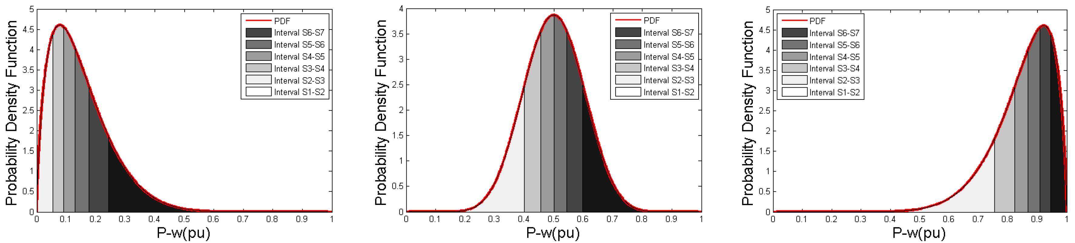
3. Scenario Generation

It is necessary to describe the uncertain vector $\mathsf{\xi }$ in Equation (2) in advance of each prediction horizon. To do this, a set of wind power scenarios for the prediction horizon representing the stochastic behaviors of the wind power need to be generated, for which we need the PDF. The wind power scenarios are generated within the range [0, 1] pu where 1 pu corresponds to the rated power value $P_{w.R}(n_w)$. $N_s$ scenarios are generated for each WS. We define $N_s-1$ intervals for the wind power $P_w(n_w,n_s),n_s=1,\cdots ,N_s$, such that:

$$\mathrm{Pr}\{P_w\left(n_w,n_s\right)-P_w\left(n_w,(n_s-1)\right)\}=\frac{1}{N_s-1},\mathrm{for}{n}_s\ge 2$$

(3)

where Pr is the probability operator. In this way, an equal probability between two adjacent scenarios is ensured. It is noted that (3) can be applied to any type of continuous bounded distribution as far as the area under its PDF curve equals one. Beta distribution is suggested to be highly suitable to represent the forecast errors of wind power ([36,37,38]). Although Beta distribution cannot model the fat tail of the forecast errors perfectly [38], due to its variable kurtosis [38], it is still more suitable than the Gaussian distribution and gives reasonably accurate results [38,39]. Beta PDF has been used in many recent studies [40,41,42,43] and therefore is chosen in this paper to represent wind power forecast errors. The PDF of the Beta distribution is defined as [36]:

$$\mathsf{\rho }\left(y,\mathsf{\alpha }(n_w),\mathsf{\beta }(n_w)\right)=y^{\mathsf{\alpha }(n_w)-1}{(1-y)}^{\mathsf{\beta }(n_w)-1},0\le y\le 1$$

(4)

where $\mathsf{\alpha }(n_w),\mathsf{\beta }(n_w)$ are the first and second shape parameters of the Beta distribution. The corresponding probability distribution function is expressed as:

$$F_{PDF}\left(P_w(n_w,n_s),\mathsf{\alpha }(n_w),\mathsf{\beta }(n_w)\right)={\displaystyle \underset{0}{\overset{P_w(n_w,n_s)}{\int }}\mathsf{\rho }\left(y,\mathsf{\alpha }(n_w),\mathsf{\beta }(n_w)\right)}dy$$

(5)

As a result, the probability in the interval between 0 and scenario $n_s$ is $\frac{n_s-1}{N_s-1}$ and then the scenarios can be generated by:

$$P_w(n_w,n_s)=F_{PDF}{}^{-1}\left(\frac{n_s-1}{N_s-1}\right),\mathrm{for}{n}_s=1,\cdots ,N_s;N_s\ge 2$$

(6)

The parameters $\mathsf{\alpha }(n_w),\mathsf{\beta }(n_w)$ can be determined by [38]:

$$\mathsf{\alpha }(n_w)=\left(\frac{1-P_{w.M}(n_w)}{{\left({\mathsf{\sigma }}_w(n_w)\right)}^2}-\frac{1}{P_{w.M}(n_w)}\right){\left(P_{w.M}(n_w)\right)}^2$$

(7)

$$\mathsf{\beta }(n_w)=\mathsf{\alpha }(n_w)\left(\frac{1}{P_{w.M}(n_w)}-1\right)$$

(8)

where $P_{w.M}(n_w)$ and ${\mathsf{\sigma }}_w(n_w)$ are the values of the mean and standard deviation of the wind power generation, respectively. For the RT-OPF, we take the forecasted values available before each prediction horizon, as $P_{w.M}(n_w)$. It is noted that the value of ${\mathsf{\sigma }}_w(n_w)$ cannot be forecasted, but it can be evaluated from historical data.

Figure 1 illustrates the generated scenarios for three forecasted wind power values when $N_s=7$ and ${\mathsf{\sigma }}_w=0.1$. It can be seen that this scenario generation method leads to more scenarios near the mean value. The scenarios generated are the boundaries of intervals. In this way, the scenarios cover the whole range [0, 1] (i.e., from zero to the rated power). Consequently, our RT-OPF can deal with any actual wind power generation (also see Section 4.2). It is noted that the scenarios here are not those from the Latin hypercube sampling method where the scenarios are randomly generated inside each interval [44]. In addition, it is noted that this scenario generation method is a significant improvement to that used in [30,31] where the scenarios were generated based on a constant width of intervals which cannot cover the whole range when a limited number of scenarios is chosen. For a power system with $N_w$ WSs, the total number of scenario combinations $N_c$ is:

$$N_c={\left(N_s\right)}^{N_w}$$

(9)

Thus, we need to define the power scenarios for individual WSs $P_w(n_w,n_s),n_s=1,\cdots ,N_s$, and the combinations of the scenarios for all WSs, $P_w(n_c),n_c=1,\cdots ,N_c$ (i.e., each combination is a vector), respectively. According to (9), when the number of WSs increases, the number of scenario combinations increases exponentially. In this case, parallel computing seems not reasonable to address the computational problem which is expectedly solved by the next generation of hardware and software, considering the rapid advancement of the computer technology. All scenarios finally generated for the power system is given in

Table 1. The list of wind power scenario combinations for all WSs.

nc	Scenario Combination
	Pw(nw,ns)	Pw(nw,ns)	…	Pw(nw,ns)	Pw(nw,ns)
	nw = 1	nw = 2		nw = Nw − 1	nw = Nw
1	Pw(1,Ns)	Pw(2,Ns)	…	Pw((Nw – 1),Ns)	Pw(Nw,Ns)
2	Pw(1,Ns)	Pw(2,Ns)	...	Pw((Nw – 1),Ns)	Pw(Nw,(Ns − 1))
. . .	. . .	. . .	. . .	. . .	. . .
Nc − 1	Pw(1,1)	Pw(2,1)	…	Pw((Nw – 1),1)	Pw(Nw,2)
Nc	Pw(1,1)	Pw(2,1)	…	Pw((Nw – 1),1)	Pw(Nw,1)

. The rules based on which the scenario combinations are sorted from the first row to row $N_c$ is further cleared by graphical examples in Figure 2. It is noted that the scenarios are listed from the highest to the least wind power values, due to the reason described in Section 4.2. To the best of the authors’ knowledge, the integration of such a scenario generation method into a RT-OPF framework has not yet been considered.

4. Solution Framework

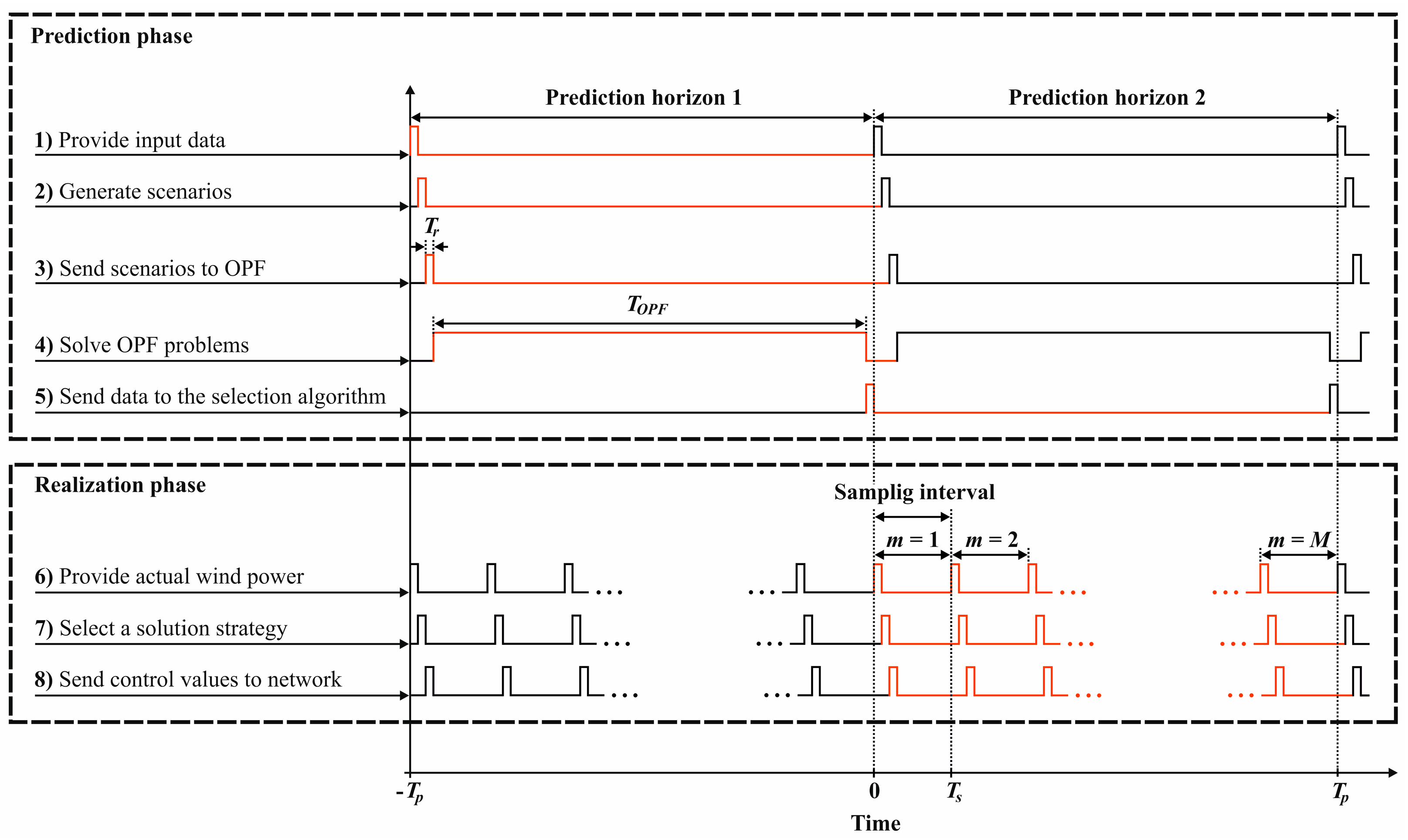
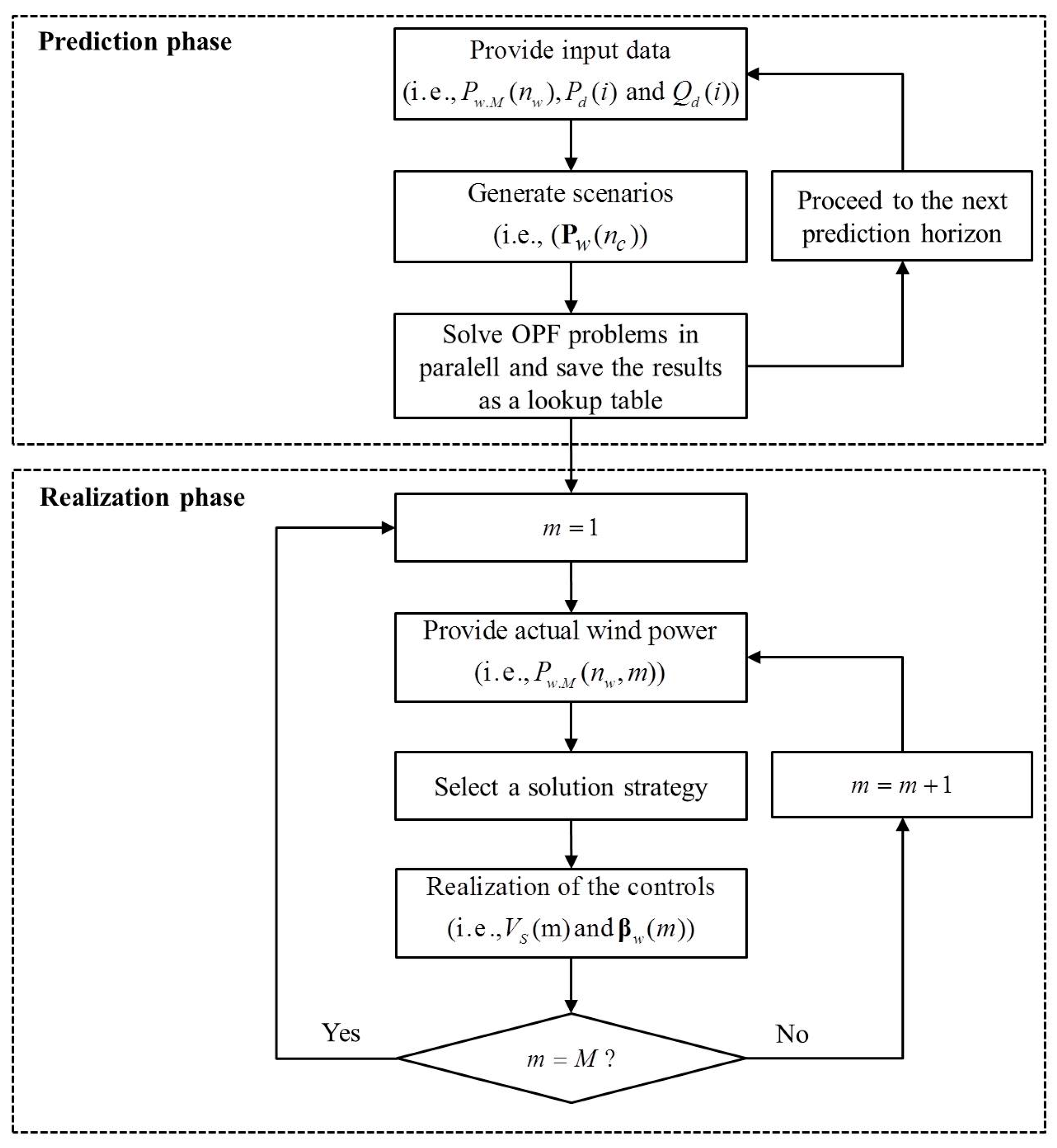
4.1. Prediction Phase

The task of the prediction phase is to solve the OPF problems corresponding to the $N_c$ scenario combinations of wind power (see Table 1) for each prediction horizon. The active and reactive power demand at bus $i$, denoted as ($P_d(i),Q_d(i)$) as well as the active and reactive energy prices ($Pric{e}_P,Pric{e}_Q$) are assumed to be constant in the short prediction horizon. But they may change from horizon to horizon. In addition, the power system model/structure is considered to be as in [5,45] and fixed in the prediction phase. The OPF problem defined in Equation (2) is formulated here in more detail for each scenario combination $n_c,(n_c=1,\cdots ,N_c)$:

$$\underset{{\mathsf{\beta }}_w(i,n_c),V_S(n_c)}{\max }f(n_c)=f_1(n_c)-f_2(n_c)-f_3(n_c)-f_4(n_c)$$

(10)

where:

$$f_1(n_c)=Pric{e}_P{\displaystyle \sum _{i=1}^{N_{bus}}{P}_w(i,n_c){\mathsf{\beta }}_w(i,n_c)}$$

(11)

$$f_2(n_c)=Pric{e}_P{P}_{loss}(n_c)$$

(12)

$$f_3(n_c)=Pric{e}_P{P}_S(n_c)$$

(13)

$$f_4(n_c)=Pric{e}_Q{Q}_S(n_c)$$

(14)

The objective function in Equation (10) aims to maximize the total revenue from the wind power $f_1(n_c)$, and meanwhile to minimize the total cost of the active energy losses in the grid $f_2(n_c)$, the cost of the active energy at slack bus $f_3(n_c)$, and the cost of the reactive energy at slack bus $f_4(n_c)$. Here, $P_{loss}(n_c)$ is the grid total active power losses [5] for scenario combination $n_c$. $P_w(i,n_c)$ is the active power of WS located at bus $i$ for scenario combination $n_c$. $P_S(n_c)$ and $Q_S(n_c)$ are the active and reactive power injected at slack bus, respectively (i.e., the imported active and reactive energy from an upstream high-voltage (HV) network). The vector of discrete decision variables $l$, in Equation (2), consists of slack bus voltage $V_S(n_c)$, representing the controller reference of tap positions of the on-load tap changer. The vector of continuous decision variables $u$ includes the curtailment factors of wind power for each WS, ${\mathsf{\beta }}_w(i,n_c)$. Here, $(0\le {\mathsf{\beta }}_w(i,n_c)\le 1)$, where ${\mathsf{\beta }}_w=1$ when no curtailment and ${\mathsf{\beta }}_w<1$ otherwise [5].

The objective function of Equation (10) is subject to the active and reactive power flow equations at the buses:

$$f_P(n_c)+P_d(i)-P_w(i,n_c){\mathsf{\beta }}_w(i,n_c)-P_S(n_c)=0,i\in sb$$

(15)

$$f_Q(n_c)+Q_d(i)-Q_S(n_c)=0,i\in sb$$

(16)

where $f_P(n_c)$ and $f_Q(n_c)$ are the network active and reactive power functions [5] for scenario combination $n_c$, respectively. $P_S(n_c)$ and $Q_S(n_c)$ are the active and reactive power terms included only for slack bus, respectively. In addition, the following inequality constraints should be held:

Bounds of active and reactive power at slack bus:

$${\left(P_S(n_c)\right)}^2+{\left(Q_S(n_c)\right)}^2\le {\left(S_{S.\max }\right)}^2$$

(17)

$$-{\mathsf{\gamma }}_{Ps,rev}{S}_{S.\max }\le P_S(n_c)\le S_{S.\max },0\le {\mathsf{\gamma }}_{Ps,rev}\le 1$$

(18)

$$-{\mathsf{\gamma }}_{Qs,rev}{S}_{S.\max }\le Q_S(n_c)\le S_{S.\max },0\le {\mathsf{\gamma }}_{Qs,rev}\le 1$$

(19)

Voltage bounds of buses:

$$V_{\min }(i)\le V(i,n_c)\le V_{\max }(i),i\in sb;i\ne 1$$

(20)

$$V_{S.\min }\le V_S(n_c)\le V_{S.\max }$$

(21)

$$V_S(n_c)=1+\Delta V_S(n_c),\Delta V_S(n_c)=\{-0.1,-0.09,\cdots ,0.09,0.1\}$$

(22)

Feeder sections limits:

$$S(i,j,n_c)\le S_{l.\max }(i,j),i,j\in sb;i\ne j$$

(23)

and the limits of the curtailment factors:

$$0\le \mathsf{\beta }(i,n_c)\le 1$$

(24)

In Equations (18) and (19), the parameters ${\mathsf{\gamma }}_{Ps,rev}$ and ${\mathsf{\gamma }}_{Qs,rev}$ define the percentage of the allowable reverse active and reactive power to an upstream HV network. For instance, if ${\mathsf{\gamma }}_{Ps,rev}=1$, active power exported to the HV network is fully allowed and if ${\mathsf{\gamma }}_{Ps,rev}=0$, no active power export is allowed. In addition, based on Equations (21) and (22), for scenario combination $n_c$, an optimal value of slack bus voltage $V_S(n_c)$ is obtained by selecting the best $\Delta V_S(n_c)$ which is a discrete variable. Therefore, the formulation of Equations (10)–(24) leads to a high-dimensional, MINLP problem for each scenario combination $n_c$. The solution of this problem is obtained by using a MINLP solver. Parallel computing can be easily carried out because each scenario is independent of the other scenarios, i.e., multiple processors can be used each of which are responsible for a number of the MINLP OPF problems. The solutions of the MINLP OPF problems lead to a lookup table providing options of operation strategies, one of which will be selected for the grid operation in the realization phase.

4.2. Realization Phase

The lookup table provides $N_c$ solutions corresponding to the scenario combinations generated based on forecasted wind power $P_{w.M}(n_w)$. The actually generated wind power values of the WSs are available at each sampling interval $m$. For each sampling interval, one of the solutions in the lookup table will be selected and the corresponding control values realized to the network. The selection is made by comparing the actual wind power $P_{w.A}(n_w,m)$ with the wind power scenarios of each WS $P_w(n_w,n_s)$, based on the following Algorithm 1:

Algorithm 1 Comparing and selection of wind power

for each WS $n_w=1,\cdots ,N_w$ and $n_s\ge 2$

$\begin{array}{l}\mathrm{If}{P}_w(n_w,(n_s-1))<P_{w.A}(n_w,m)\le P_w(n_w,n_s)\\ \mathrm{then}\mathrm{consider}{P}_{w.A}(n_w,m)\mathrm{as}{P}_w(n_w,n_s)\end{array}$

end

Achieve $P_w(n_c)$

Based on $n_c$, set ${\mathsf{\beta }}_w(m)={\mathsf{\beta }}_w(n_c)\mathrm{and}{V}_S(m)=V_S(n_c)$

This means, for each WS $n_w$, if $P_{w.A}(n_w,m)$ is not equal to $P_w(n_w,(n_s-1))$, then consider it to be the nearest higher scenario. This is because a higher wind power associates with a lower curtailment factor, leading to a feasible operation strategy. Since the scenarios generated in the prediction phase cover the whole range [0, 1], for any actual value of wind power, there is a higher or equal scenario corresponding to an optimal operation strategy. It should be noted that the decision made in this way also has a certain degree of built-in conservativeness, so that feasibility of the selected solution to be realized to the grid can be ensured. This conservativeness will be decreased if more scenarios for each WS are used. But then the number of MINLP problems to be solved will be increased correspondingly.

4.3. Implementation of the Real-Time Optimal Power Flow Framework

The RT-OPF framework of the proposed prediction-realization approach is implemented as shown in Figure 3 where the execution steps are shown by the numbers. It consists of following eight steps:

(1)

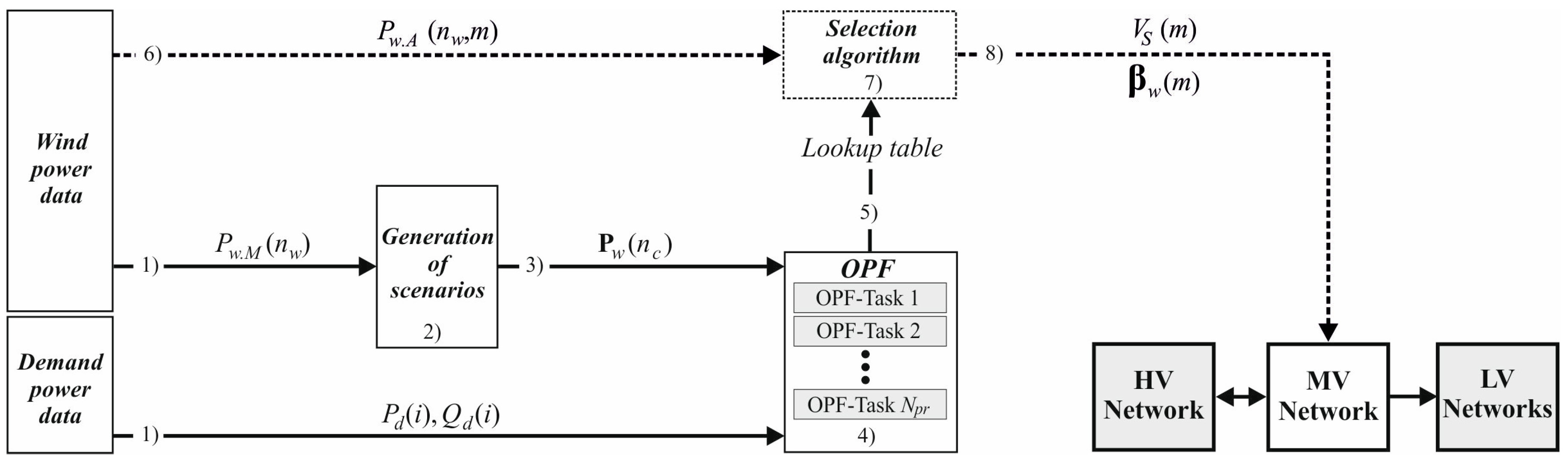
For the current prediction horizon, provide the forecasted active $P_d(i)$ and reactive $Q_d(i)$ demand power and wind power $P_{w.M}(n_w)$.

(2)

Generate $N_c$ wind power scenario combinations based on the Beta distribution as described in Section 3.

(3)

Send the generated scenarios as inputs to formulate $N_c$ MINLP OPF problems.

(4)

Solve the $N_c$ MINLP OPF problems with parallel computing.

(5)

Send the solution results as a lookup table to the selection algorithm.

(6)

Provide the actual wind power of WSs, $P_{w.A}(n_w,m)$, available at the current sampling time $m$ (for $m=1,\cdots ,M$), to the selection algorithm.

(7)

Select one of the solutions from the lookup table based on $P_{w.A}(n_w,m)$ and the selection algorithm (see Section 4.2).

(8)

Send the values of the controls $V_S(m)$ and ${\mathsf{\beta }}_w(m)$ to the grid.

Steps 1–5, as shown with solid lines in Figure 3, correspond to the prediction phase, while steps 6–8, presented with dashed lines, denote the realization phase. Step 8 means that, with an optimal value of the slack bus voltage, an optimal amount of wind power is penetrated to the grid in the current sampling time $m$. When $m=M$, the computation proceeds to the next prediction horizon.

To online realize the computation framework described above, it is necessary to ensure all 8 steps to be completed inside the time slot of $T_p$. The implementation is illustrated in Figure 4, showing two consecutive prediction horizons. In Figure 4, the red lines indicate the execution of the eight tasks along the time. It means when the optimal strategies for the current prediction horizon are realized to the network, the solutions for the upcoming prediction horizon are prepared.

In Figure 4, $T_r$ denotes the length of the time reserved for data management (for our case study $T_r=2s$). For steps 1, 3, 5, 6, and 8, $T_r$ means the communication (i.e., sending/receiving data) time. In steps 2, 4, and 7, $T_r$ means the time for processing data after receiving the corresponding inputs. $T_{OPF}$ is the time to solve the $N_c$ OPF problems, which takes the largest part of the time horizon.

$T_p$ is the prediction horizon for which the forecasted data is available and its length should be the summation of the lengths of all the tasks (including OPF computations as shown in Figure 4) in the prediction phase:

$$T_p=4T_r+T_{OPF}$$

(25)

Here, the greatest time slot is allocated to the computation of the OPF problems corresponding to the generated scenarios (i.e., $T_{OPF}$). It means that, at the end of the prediction phase, the OPF results must be ready for the selection algorithm in the realization phase.

The sampling time $T_s$ in which the actual values of wind power are available, could be very short (even less than a second). However, since the realization is also performed at every $T_s$, the length of $T_s$ should be realistic in order not to damage devices by too frequent control actions in very short time intervals. On the other hand, based on Equation (1), $T_s$ theoretically can be equal to $T_p$ (i.e., $M=1$). However, long sampling intervals could not response the intermittency of the wind power.

The wind power spectrum has been investigated for a long time. Using short term and long term records, the Van der Hoven spectrum [46] shows the diurnal and turbulence effects of wind power. It confirms that there are considerable wind power discrepancies in short term (e.g., 1 min) periods. The spectrum has been also studied to evaluate and improve wind power prediction [47,48]. However, in this study, we assume that the values of wind power prediction are provided by a forecast center. The time period over which the forecasted value is updated, is defined as the prediction horizon. In our case study, the forecasted wind power value is assumed to be available every two minutes. Thus we define the length of the prediction horizon as two minutes. The forecasted wind power profiles for one day are taken from [31] for the case study. Indeed, this is the reason that the blocks ‘Wind power data’ and ‘Demand power data’ are not included in the ‘8 steps’ of the framework in Figure 3. This means that the way how the wind and power demand power data is obtained is not considered in this study.

As mentioned in Section 3, parallel computing is used for solving the individual MINLP problems by multiple processors, each of which solves an equal number of the optimization problems. Therefore, the time needed for the solutions to be available is the maximum time taken by the processors. But we need to allocate $T_{OPF}$ large enough to ensure that none of the processors exceeds this limit. The proposed RT-OPF framework is further described by a flowchart in Figure 5. The flowchart shows the prediction and realization phases.

5. Case Study

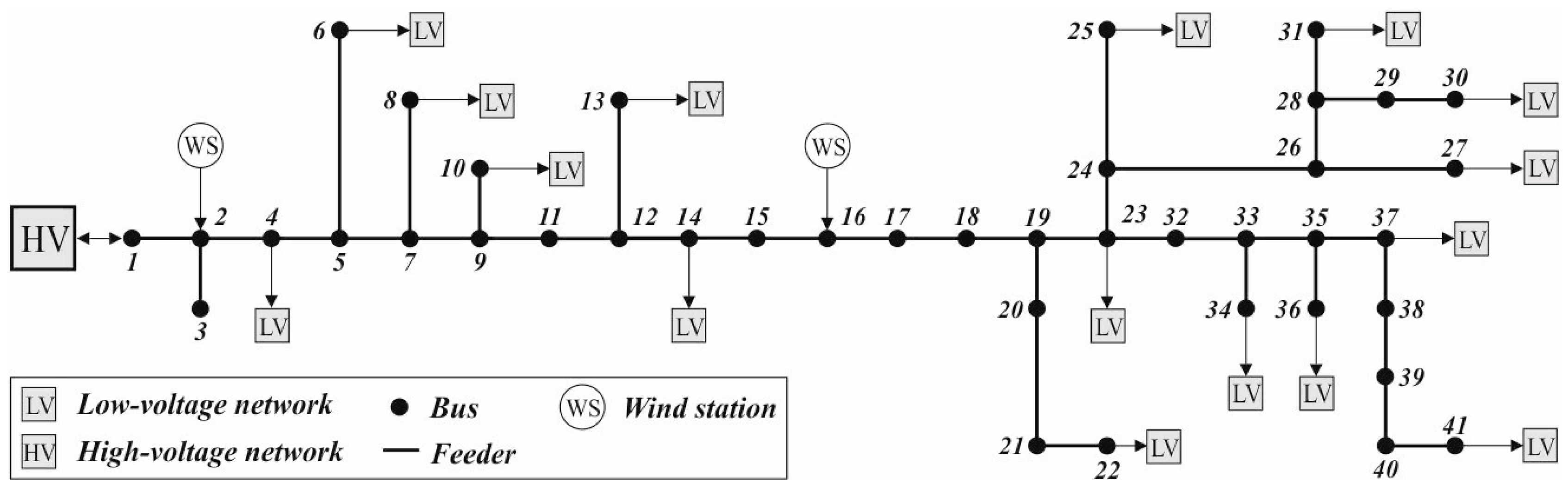
5.1. Network and Input Data

The network for the case study is taken from [49,50]. It is a 41-bus, 27.6 kV typical rural DN, as shown in Figure 6. The peak power demand is 16.25 MVA [5] and the substation rating is 20 MVA. Two WSs each with $P_{w.R}=10\mathrm{MW}$ and unity power factors are located at buses 2 and 16, as shown in Figure 6. The WSs are subject to different wind profiles which make the problem more complicated. The bus number 1 is considered as the slack bus with zero voltage angle [49,50]. The active and reactive energy prices are adapted and fixed with $1.67\$/\mathrm{MW}.T_p$ and $0.4\$/\mathrm{Mvar}.T_p$ [31,49], respectively. We assume that the forecasted and measured values of wind power generation are available in every 120 and 20 s, respectively. Therefore, the length of the prediction horizon $T_p$ and the length of the sampling time $T_s$ are taken as 120 and 20 s, respectively. For generating wind scenarios, we take $N_s=7$ which means we consider seven scenarios for each of the two WSs, leading to $N_c=49$ MINLP OPF problems. To implement parallel computing, we use seven processors to solve the 49 problems (i.e., seven scenario combinations are allocated to each processor). The computations are carried out on a server with 2 Intel Xeon X5690, CPU 3.47 GHz (six cores, 12 threads) and 64 GB random access memory (RAM). The problem is formulated and coded in the general algebraic modeling system (GAMS) [51] framework and the resulting problem solved by the MINLP solver BONMIN [52], using the usual flat start [5]. Based on the BONMIN manual [52], the algorithms are exact when both the objective function and the constraints are convex, otherwise they are heuristics. It is also noted that there are some possible model status messages in GAMS. In solving our MINLP problems, we always got the message No. 8 (integer solution), meaning that a feasible solution has been found to problems with discrete variables, see details in [51]. However, the solution achieved in this way should be considered as a local solution, since the power flow equations are nonconvex.

The active $P_d$ and reactive $Q_d$ power demand are assumed to follow the hourly IEEE-RTS fall season’s days [49]. However, inside each hour, the demand profiles are generated for every bus at every 120 s by adding normally distributed random values (with ${\mathsf{\mu }}_d(i)=0$ and ${\mathsf{\sigma }}_d(i)=0.01$) to the hourly values [31]. The resulting demand trajectories for one day are shown in Figure 7a.

In the reality, the forecasted and actual wind power profiles can be acquired from environmental data centers and online measurements, respectively. The forecasted wind power profiles for one day are taken from [31] and shown as the red-dashed curves in Figure 7b,c. The actual wind power $P_{w.A}(n_w,m)$ for the two WSs are generated at each 20 s using the Beta distribution with the shape parameters $\mathsf{\alpha }(n_w)$ and $\mathsf{\beta }(n_w)$ corresponding to the forecasted wind power, where ${\mathsf{\sigma }}_w(n_w)=0.1\mathrm{pu}=1\mathrm{MW}$ based on Equations (7) and (8). The resulting curves for the two WSs are shown in Figure 7b,c.

5.2. Test Cases

In the case study, possible reverse power flow is considered for the proposed RT-OPF framework. We define the forward and reverse active as well as reactive energy at the slack bus as follows:

• Forward energy flow: The forward active and reactive energy from the HV network to the MV network is to be minimized based on an energy price model.
• Reverse energy flow: The reverse power flow could have impacts on voltage profiles [53] of the upper-level network and may result in specific operational limits being exceeded at the congested primary substations [54]. However, reverse flows have been considered in many studies [45,55,56,57,58] and in reality, they are likely to happen. Therefore, in this paper we consider the cases with and without reverse power flows.

Furthermore, in the optimization problem formulation, the slack bus voltage can be either a parameter with a fixed value or a discrete free variable. Based on these considerations, we carry out RT-OPF for four different cases defined as follows:

Case (1):

Both reverse active and reactive power to the upstream HV network is not allowed (i.e., ${\mathsf{\gamma }}_{Ps,rev}={\mathsf{\gamma }}_{Qs,rev}=0$), and with a fixed value of the slack bus voltage ($V_S(m)=V_S(n_c)=1\mathrm{pu}$).

Case (2):

Both reverse active and reactive power to upstream HV network is not allowed (i.e., ${\mathsf{\gamma }}_{Ps,rev}={\mathsf{\gamma }}_{Qs,rev}=0$), and with the slack bus voltage as a discrete free variable.

Case (3):

Both reverse active and reactive power to upstream HV network is allowed (i.e., ${\mathsf{\gamma }}_{Ps,rev}={\mathsf{\gamma }}_{Qs,rev}=1$), and with a fixed value of the slack bus voltage (i.e., $V_S(m)=V_S(n_c)=1\mathrm{pu}$).

Case (4):

Both reverse active and reactive power to upstream HV network is allowed (i.e., ${\mathsf{\gamma }}_{Ps,rev}={\mathsf{\gamma }}_{Qs,rev}=1$), and with the slack bus voltage as a discrete free variable.

5.3. Results and Discussions

We run the RT-OPF for one day for the aforementioned four cases using the same network in Figure 6 and the input data in Figure 7. To illustrate the prediction phase and the realization phase, we firstly take the first prediction horizon (i.e., $t\in [0,120\mathrm{s}]$) as an example. The forecasted values of wind power for the two WSs in the first prediction horizon are $P_{w.M}(1)=3.8\mathrm{MW}$ and $P_{w.M}(2)=7.05\mathrm{MW}$. The wind power scenario combinations and the corresponding results for the four cases in the first prediction horizon are shown in

Table 2. Lookup table for the first prediction horizon (with P_w.M(1) = 3.8 MW, P_w.M(2) = 7.05 MW) for Case 1.

Scenario Combination			Optimal Results
nc	Pw(nw,ns) (MW) nw = 1	Pw(nw,ns) (MW) nw = 2	βw(1) -	βw(2) -	Vs (pu)	PS (MW)	QS (Mvar)
1	Pw(1,7) = 10	Pw(2,7) = 10	0.379	0.288	1	0	2.375
2	Pw(1,7) = 10	Pw(2,6) = 8.04	0.379	0.358	1	0	2.375
3	Pw(1,7) = 10	Pw(2,5) = 7.55	0.379	0.382	1	0	2.375
4	Pw(1,7) = 10	Pw(2,4) = 7.13	0.379	0.404	1	0	2.375
5	Pw(1,7) = 10	Pw(2,3) = 6.67	0.379	0.432	1	0	2.375
6	Pw(1,7) = 10	Pw(2,2) = 6.07	0.379	0.475	1	0	2.375
7	Pw(1,7) = 10	Pw(2,1) = 0	0.669	1	1	0	2.406
8	Pw(1,6) = 4.79	Pw(2,7) = 10	0.792	0.288	1	0	2.375
9	Pw(1,6) = 4.79	Pw(2,6) = 8.04	0.792	0.358	1	0	2.375
10	Pw(1,6) = 4.79	Pw(2,5) = 7.55	0.792	0.382	1	0	2.375
11	Pw(1,6) = 4.79	Pw(2,4) = 7.13	0.792	0.404	1	0	2.375
12	Pw(1,6) = 4.79	Pw(2,3) = 6.67	0.792	0.432	1	0	2.375
13	Pw(1,6) = 4.79	Pw(2,2) = 6.07	0.792	0.475	1	0	2.375
14	Pw(1,6) = 4.79	Pw(2,1) = 0	1	1	1	1.9	2.419
15	Pw(1,5) = 4.22	Pw(2,7) = 10	0.899	0.288	1	0	2.375
16	Pw(1,5) = 4.22	Pw(2,6) = 8.04	0.899	0.358	1	0	2.375
17	Pw(1,5) = 4.22	Pw(2,5) = 7.55	0.899	0.382	1	0	2.375
18	Pw(1,5) = 4.22	Pw(2,4) = 7.13	0.899	0.404	1	0	2.375
19	Pw(1,5) = 4.22	Pw(2,3) = 6.67	0.899	0.432	1	0	2.375
20	Pw(1,7) = 4.22	Pw(2,2) = 6.07	0.899	0.475	1	0	2.375
21	Pw(1,5) = 4.22	Pw(2,1) = 0	1	1	1	2.476	2.427
22	Pw(1,4) = 3.77	Pw(2,7) = 10	1	0.29	1	0	2.375
23	Pw(1,4) = 3.77	Pw(2,6) = 8.04	1	0.361	1	0	2.375
24	Pw(1,4) = 3.77	Pw(2,5) = 7.55	1	0.385	1	0	2.375
25	Pw(1,4) = 3.77	Pw(2,4) = 7.13	1	0.407	1	0	2.375
26	Pw(1,4) = 3.77	Pw(2,3) = 6.67	1	0.435	1	0	2.375
27	Pw(1,4) = 3.77	Pw(2,2) = 6.07	1	0.478	1	0	2.375
28	Pw(1,4) = 3.77	Pw(2,1) = 0	1	1	1	2.927	2.435
29	Pw(1,3) = 3.33	Pw(2,7) = 10	1	0.334	1	0	2.376
30	Pw(1,3) = 3.33	Pw(2,6) = 8.04	1	0.416	1	0	2.376
31	Pw(1,3) = 3.33	Pw(2,5) = 7.55	1	0.443	1	0	2.376
32	Pw(1,3) = 3.33	Pw(2,4) = 7.13	1	0.469	1	0	2.376
33	Pw(1,3) = 3.33	Pw(2,3) = 6.67	1	0.501	1	0	2.376
34	Pw(1,3) = 3.33	Pw(2,2) = 6.07	1	0.551	1	0	2.376
35	Pw(1,3) = 3.33	Pw(2,1) = 0	1	1	1	3.370	2.444
36	Pw(1,2) = 2.81	Pw(2,7) = 10	1	0.387	1	0	2.379
37	Pw(1,2) = 2.81	Pw(2,6) = 8.04	1	0.481	1	0	2.379
38	Pw(1,2) = 2.81	Pw(2,5) = 7.55	1	0.512	1	0	2.379
39	Pw(1,2) = 2.81	Pw(2,4) = 7.13	1	0.542	1	0	2.379
40	Pw(1,2) = 2.81	Pw(2,3) = 6.67	1	0.58	1	0	2.379
41	Pw(1,2) = 2.81	Pw(2,2) = 6.07	1	0.637	1	0	2.379
42	Pw(1,2) = 2.81	Pw(2,1) = 0	1	1	1	3.895	2.457
43	Pw(1,1) = 0	Pw(2,7) = 10	1	0.67	1	0	2.429
44	Pw(1,1) = 0	Pw(2,6) = 8.04	1	0.833	1	0	2.429
45	Pw(1,1) = 0	Pw(2,5) = 7.55	1	0.887	1	0	2.429
46	Pw(1,1) = 0	Pw(2,4) = 7.13	1	0.939	1	0	2.429
47	Pw(1,1) = 0	Pw(2,3) = 6.67	1	1	1	0.025	2.428
48	Pw(1,1) = 0	Pw(2,2) = 6.07	1	1	1	0.619	2.414
49	Pw(1,1) = 0	Pw(2,1) = 0	1	1	1	6.744	2.554

,

Table 3. Lookup table for the first prediction horizon (with P_w.M(1) = 3.8 MW, P_w.M(2) = 7.05 MW) for Case 2.

Scenario Combination			Optimal Results
nc	Pw(nw,ns) (MW) nw = 1	Pw(nw,ns) (MW) nw = 2	βw(1) -	βw(2) -	Vs (pu)	PS (MW)	QS (Mvar)
1	Pw(1,7) = 10	Pw(2,7) = 10	0.379	0.288	1.06	0	2.352
2	Pw(1,7) = 10	Pw(2,6) = 8.04	0.379	0.359	1.06	0	2.352
3	Pw(1,7) = 10	Pw(2,5) = 7.55	0.379	0.382	1.06	0	2.352
4	Pw(1,7) = 10	Pw(2,4) = 7.13	0.379	0.405	1.06	0	2.352
5	Pw(1,7) = 10	Pw(2,3) = 6.67	0.379	0.432	1.06	0	2.352
6	Pw(1,7) = 10	Pw(2,2) = 6.07	0.379	0.475	1.06	0	2.352
7	Pw(1,7) = 10	Pw(2,1) = 0	0.668	1	1.06	0	2.38
8	Pw(1,6) = 4.79	Pw(2,7) = 10	0.791	0.288	1.06	0	2.352
9	Pw(1,6) = 4.79	Pw(2,6) = 8.04	0.791	0.359	1.06	0	2.352
10	Pw(1,6) = 4.79	Pw(2,5) = 7.55	0.791	0.382	1.06	0	2.352
11	Pw(1,6) = 4.79	Pw(2,4) = 7.13	0.791	0.405	1.06	0	2.352
12	Pw(1,6) = 4.79	Pw(2,3) = 6.67	0.791	0.433	1.06	0	2.352
13	Pw(1,6) = 4.79	Pw(2,2) = 6.07	0.791	0.475	1.06	0	2.352
14	Pw(1,6) = 4.79	Pw(2,1) = 0	1.000	1	1.06	1.896	2.391
15	Pw(1,5) = 4.22	Pw(2,7) = 10	0.898	0.288	1.06	0	2.352
16	Pw(1,5) = 4.22	Pw(2,6) = 8.04	0.898	0.359	1.06	0	2.352
17	Pw(1,5) = 4.22	Pw(2,5) = 7.55	0.898	0.382	1.06	0	2.352
18	Pw(1,5) = 4.22	Pw(2,4) = 7.13	0.898	0.405	1.06	0	2.352
19	Pw(1,5) = 4.22	Pw(2,3) = 6.67	0.898	0.433	1.06	0	2.352
20	Pw(1,7) = 4.22	Pw(2,2) = 6.07	0.898	0.475	1.06	0	2.352
21	Pw(1,5) = 4.22	Pw(2,1) = 0	1	1	1.06	2.471	2.398
22	Pw(1,4) = 3.77	Pw(2,7) = 10	1	0.29	1.06	0	2.352
23	Pw(1,4) = 3.77	Pw(2,6) = 8.04	1	0.361	1.06	0	2.352
24	Pw(1,4) = 3.77	Pw(2,5) = 7.55	1	0.384	1.06	0	2.352
25	Pw(1,4) = 3.77	Pw(2,4) = 7.13	1	0.407	1.06	0	2.352
26	Pw(1,4) = 3.77	Pw(2,3) = 6.67	1	0.435	1.06	0	2.352
27	Pw(1,4) = 3.77	Pw(2,2) = 6.07	1	0.478	1.06	0	2.352
28	Pw(1,4) = 3.77	Pw(2,1) = 0	1	1	1.07	2.921	2.401
29	Pw(1,3) = 3.33	Pw(2,7) = 10	1	0.334	1.06	0	2.353
30	Pw(1,3) = 3.33	Pw(2,6) = 8.04	1	0.416	1.06	0	2.353
31	Pw(1,3) = 3.33	Pw(2,5) = 7.55	1	0.443	1.06	0	2.353
32	Pw(1,3) = 3.33	Pw(2,4) = 7.13	1	0.469	1.06	0	2.353
33	Pw(1,3) = 3.33	Pw(2,3) = 6.67	1	0.501	1.06	0	2.353
34	Pw(1,3) = 3.33	Pw(2,2) = 6.07	1	0.551	1.06	0	2.353
35	Pw(1,3) = 3.33	Pw(2,1) = 0	1	1	1.07	3.364	2.409
36	Pw(1,2) = 2.81	Pw(2,7) = 10	1	0.386	1.06	0	2.355
37	Pw(1,2) = 2.81	Pw(2,6) = 8.04	1	0.480	1.06	0	2.355
38	Pw(1,2) = 2.81	Pw(2,5) = 7.55	1	0.512	1.06	0	2.355
39	Pw(1,2) = 2.81	Pw(2,4) = 7.13	1	0.542	1.06	0	2.355
40	Pw(1,2) = 2.81	Pw(2,3) = 6.67	1	0.579	1.06	0	2.355
41	Pw(1,2) = 2.81	Pw(2,2) = 6.07	1	0.636	1.06	0	2.355
42	Pw(1,2) = 2.81	Pw(2,1) = 0	1	1	1.07	3.888	2.419
43	Pw(1,1) = 0	Pw(2,7) = 10	1	0.669	1.06	0	2.4
44	Pw(1,1) = 0	Pw(2,6) = 8.04	1	0.832	1.06	0	2.4
45	Pw(1,1) = 0	Pw(2,5) = 7.55	1	0.886	1.06	0	2.4
46	Pw(1,1) = 0	Pw(2,4) = 7.13	1	0.938	1.06	0	2.4
47	Pw(1,1) = 0	Pw(2,3) = 6.67	1	1	1.06	0.02	2.399
48	Pw(1,1) = 0	Pw(2,2) = 6.07	1	1	1.06	0.615	2.387
49	Pw(1,1) = 0	Pw(2,1) = 0	1	1	1.07	6.731	2.504

,

Table 4. Lookup table for the first prediction horizon (with P_w.M(1) = 3.8 MW, P_w.M(2) = 7.05 MW) for Case 3.

Scenario Combination			Optimal Results
nc	Pw(nw,ns) (MW) nw = 1	Pw(nw,ns) (MW) nw = 2	βw(1) -	βw(2) -	Vs (pu)	PS (MW)	QS (Mvar)
1	Pw(1,7) = 10	Pw(2,7) = 10	1	1	1	−13.034	3.091
2	Pw(1,7) = 10	Pw(2,6) = 8.04	1	1	1	−11.167	2.863
3	Pw(1,7) = 10	Pw(2,5) = 7.55	1	1	1	−10.697	2.813
4	Pw(1,7) = 10	Pw(2,4) = 7.13	1	1	1	−10.293	2.773
5	Pw(1,7) = 10	Pw(2,3) = 6.67	1	1	1	−9.85	2.731
6	Pw(1,7) = 10	Pw(2,2) = 6.07	1	1	1	−9.27	2.681
7	Pw(1,7) = 10	Pw(2,1) = 0	1	1	1	−3.301	2.439
8	Pw(1,6) = 4.79	Pw(2,7) = 10	1	1	1	−7.96	2.755
9	Pw(1,6) = 4.79	Pw(2,6) = 8.04	1	1	1	−6.069	2.586
10	Pw(1,6) = 4.79	Pw(2,5) = 7.55	1	1	1	−5.593	2.551
11	Pw(1,6) = 4.79	Pw(2,4) = 7.13	1	1	1	−5.184	2.524
12	Pw(1,6) = 4.79	Pw(2,3) = 6.67	1	1	1	−4.736	2.497
13	Pw(1,6) = 4.79	Pw(2,2) = 6.07	1	1	1	−4.148	2.465
14	Pw(1,6) = 4.79	Pw(2,1) = 0	1	1	1	1.9	2.419
15	Pw(1,5) = 4.22	Pw(2,7) = 10	1	1	1	−7.399	2.728
16	Pw(1,5) = 4.22	Pw(2,6) = 8.04	1	1	1	−5.505	2.566
17	Pw(1,5) = 4.22	Pw(2,5) = 7.55	1	1	1	−5.029	2.533
18	Pw(1,5) = 4.22	Pw(2,4) = 7.13	1	1	1	−4.619	2.507
19	Pw(1,5) = 4.22	Pw(2,3) = 6.67	1	1	1	−4.17	2.481
20	Pw(1,7) = 4.22	Pw(2,2) = 6.07	1	1	1	−3.582	2.452
21	Pw(1,5) = 4.22	Pw(2,1) = 0	1	1	1	2.476	2.427
22	Pw(1,4) = 3.77	Pw(2,7) = 10	1	1	1	−6.959	2.708
23	Pw(1,4) = 3.77	Pw(2,6) = 8.04	1	1	1	−5.063	2.551
24	Pw(1,4) = 3.77	Pw(2,5) = 7.55	1	1	1	−4.586	2.519
25	Pw(1,4) = 3.77	Pw(2,4) = 7.13	1	1	1	−4.176	2.495
26	Pw(1,4) = 3.77	Pw(2,3) = 6.67	1	1	1	−3.726	2.47
27	Pw(1,4) = 3.77	Pw(2,2) = 6.07	1	1	1	−3.138	2.442
28	Pw(1,4) = 3.77	Pw(2,1) = 0	1	1	1	2.927	2.435
29	Pw(1,3) = 3.33	Pw(2,7) = 10	1	1	1	−6.527	2.69
30	Pw(1,3) = 3.33	Pw(2,6) = 8.04	1	1	1	−4.629	2.538
31	Pw(1,3) = 3.33	Pw(2,5) = 7.55	1	1	1	−4.151	2.508
32	Pw(1,3) = 3.33	Pw(2,4) = 7.13	1	1	1	−3.741	2.484
33	Pw(1,3) = 3.33	Pw(2,3) = 6.67	1	1	1	−3.29	2.461
34	Pw(1,3) = 3.33	Pw(2,2) = 6.07	1	1	1	−2.701	2.434
35	Pw(1,3) = 3.33	Pw(2,1) = 0	1	1	1	3.37	2.444
36	Pw(1,2) = 2.81	Pw(2,7) = 10	1	1	1	−6.015	2.670
37	Pw(1,2) = 2.81	Pw(2,6) = 8.04	1	1	1	−4.115	2.524
38	Pw(1,2) = 2.81	Pw(2,5) = 7.55	1	1	1	−3.636	2.495
39	Pw(1,2) = 2.81	Pw(2,4) = 7.13	1	1	1	−3.225	2.473
40	Pw(1,2) = 2.81	Pw(2,3) = 6.67	1	1	1	−2.774	2.451
41	Pw(1,2) = 2.81	Pw(2,2) = 6.07	1	1	1	−2.184	2.427
42	Pw(1,2) = 2.81	Pw(2,1) = 0	1	1	1	3.895	2.457
43	Pw(1,1) = 0	Pw(2,7) = 10	1	1	1	−3.239	2.591
44	Pw(1,1) = 0	Pw(2,6) = 8.04	1	1	1	−1.325	2.478
45	Pw(1,1) = 0	Pw(2,5) = 7.55	1	1	1	−0.843	2.457
46	Pw(1,1) = 0	Pw(2,4) = 7.13	1	1	1	−0.429	2.442
47	Pw(1,1) = 0	Pw(2,3) = 6.67	1	1	1	0.025	2.428
48	Pw(1,1) = 0	Pw(2,2) = 6.07	1	1	1	0.619	2.414
49	Pw(1,1) = 0	Pw(2,1) = 0	1	1	1	6.744	2.554

and

Table 5. Lookup table for the first prediction horizon (with P_w.M(1) = 3.8 MW, P_w.M(2) = 7.05 MW) for Case 4.

Scenario Combination			Optimal Results
nc	Pw(nw,ns) (MW) nw = 1	Pw(nw,ns) (MW) nw = 2	βw(1) -	βw(2)-	Vs (pu)	PS (MW)	QS (Mvar)
1	Pw(1,7) = 10	Pw(2,7) = 10	1	1	1.04	−13.057	3.022
2	Pw(1,7) = 10	Pw(2,6) = 8.04	1	1	1.05	−11.187	2.798
3	Pw(1,7) = 10	Pw(2,5) = 7.55	1	1	1.05	−10.715	2.753
4	Pw(1,7) = 10	Pw(2,4) = 7.13	1	1	1.05	−10.31	2.717
5	Pw(1,7) = 10	Pw(2,3) = 6.67	1	1	1.05	−9.866	2.679
6	Pw(1,7) = 10	Pw(2,2) = 6.07	1	1	1.05	−9.284	2.634
7	Pw(1,7) = 10	Pw(2,1) = 0	1	1	1.06	−3.306	2.409
8	Pw(1,6) = 4.79	Pw(2,7) = 10	1	1	1.05	−7.977	2.701
9	Pw(1,6) = 4.79	Pw(2,6) = 8.04	1	1	1.05	−6.079	2.547
10	Pw(1,6) = 4.79	Pw(2,5) = 7.55	1	1	1.05	−5.602	2.516
11	Pw(1,6) = 4.79	Pw(2,4) = 7.13	1	1	1.05	−5.192	2.491
12	Pw(1,6) = 4.79	Pw(2,3) = 6.67	1	1	1.05	−4.742	2.466
13	Pw(1,6) = 4.79	Pw(2,2) = 6.07	1	1	1.06	−4.155	2.432
14	Pw(1,6) = 4.79	Pw(2,1) = 0	1	1	1.06	1.896	2.391
15	Pw(1,5) = 4.22	Pw(2,7) = 10	1	1	1.05	−7.414	2.676
16	Pw(1,5) = 4.22	Pw(2,6) = 8.04	1	1	1.05	−5.515	2.529
17	Pw(1,5) = 4.22	Pw(2,5) = 7.55	1	1	1.05	−5.037	2.499
18	Pw(1,5) = 4.22	Pw(2,4) = 7.13	1	1	1.05	−4.626	2.475
19	Pw(1,5) = 4.22	Pw(2,3) = 6.67	1	1	1.05	−4.176	2.452
20	Pw(1,7) = 4.22	Pw(2,2) = 6.07	1	1	1.06	−3.588	2.42
21	Pw(1,5) = 4.22	Pw(2,1) = 0	1	1	1.06	2.471	2.398
22	Pw(1,4) = 3.77	Pw(2,7) = 10	1	1	1.05	−6.974	2.658
23	Pw(1,4) = 3.77	Pw(2,6) = 8.04	1	1	1.05	−5.072	2.515
24	Pw(1,4) = 3.77	Pw(2,5) = 7.55	1	1	1.05	−4.594	2.487
25	Pw(1,4) = 3.77	Pw(2,4) = 7.13	1	1	1.05	−4.183	2.464
26	Pw(1,4) = 3.77	Pw(2,3) = 6.67	1	1	1.06	−3.733	2.437
27	Pw(1,4) = 3.77	Pw(2,2) = 6.07	1	1	1.06	−3.143	2.412
28	Pw(1,4) = 3.77	Pw(2,1) = 0	1	1	1.07	2.921	2.401
29	Pw(1,3) = 3.33	Pw(2,7) = 10	1	1	1.05	−6.541	2.642
30	Pw(1,3) = 3.33	Pw(2,6) = 8.04	1	1	1.05	−4.637	2.504
31	Pw(1,3) = 3.33	Pw(2,5) = 7.55	1	1	1.05	−4.158	2.476
32	Pw(1,3) = 3.33	Pw(2,4) = 7.13	1	1	1.05	−3.747	2.455
33	Pw(1,3) = 3.33	Pw(2,3) = 6.67	1	1	1.06	−3.297	2.428
34	Pw(1,3) = 3.33	Pw(2,2) = 6.07	1	1	1.06	−2.706	2.405
35	Pw(1,3) = 3.33	Pw(2,1) = 0	1	1	1.07	3.364	2.409
36	Pw(1,2) = 2.81	Pw(2,7) = 10	1	1	1.05	−6.028	2.624
37	Pw(1,2) = 2.81	Pw(2,6) = 8.04	1	1	1.05	−4.122	2.491
38	Pw(1,2) = 2.81	Pw(2,5) = 7.55	1	1	1.05	−3.643	2.465
39	Pw(1,2) = 2.81	Pw(2,4) = 7.13	1	1	1.06	−3.232	2.439
40	Pw(1,2) = 2.81	Pw(2,3) = 6.67	1	1	1.06	−2.78	2.42
41	Pw(1,2) = 2.81	Pw(2,2) = 6.07	1	1	1.06	−2.189	2.398
42	Pw(1,2) = 2.81	Pw(2,1) = 0	1	1	1.07	3.888	2.419
43	Pw(1,1) = 0	Pw(2,7) = 10	1	1	1.05	−3.249	2.551
44	Pw(1,1) = 0	Pw(2,6) = 8.04	1	1	1.06	−1.332	2.443
45	Pw(1,1) = 0	Pw(2,5) = 7.55	1	1	1.06	−0.849	2.425
46	Pw(1,1) = 0	Pw(2,4) = 7.13	1	1	1.06	−0.435	2.411
47	Pw(1,1) = 0	Pw(2,3) = 6.67	1	1	1.06	0.02	2.399
48	Pw(1,1) = 0	Pw(2,2) = 6.07	1	1	1.06	0.615	2.387
49	Pw(1,1) = 0	Pw(2,1) = 0	1	1	1.07	6.731	2.504

.

The lookup tables consist of two sections: “scenario combinations” and “optimal results”. The scenario combinations are obtained as described in Section 3 and optimal results are achieved by solving the corresponding OPF problems (i.e., Equations (10)–(24)). Based on Equation (9), there are 49 scenarios in each lookup table from which one action will be selected in each sampling interval $T_s$. It is noted that the lookup tables are updated in each prediction horizon $T_p$ based on the new values of forecasted wind and demand power.

In the first sampling time interval (i.e., $t\in [0,20\mathrm{s}]$), the real wind power are $P_{w.A}(1,1)=3.74\mathrm{MW}$ and $P_{w.A}(2,1)=4.17\mathrm{MW}$, respectively. Therefore, the selection algorithm (shown as Step 7 in Figure 3) selects the scenario combination 27 which corresponds to the level higher than the real value of wind power for both WSs. Then the control strategy corresponding to this scenario combination will be realized to the grid.

It can be seen in Table 2 and Table 3 that, for this prediction horizon, the active power at the slack bus is zero when the wind power of WSs is high. This is because of the low total active power demand (6.65 MW) and high active wind power generation. In addition, the high wind power generation leads to high curtailment (i.e., low values of the curtailment factors) to ensure feasibility. In contrast, if reverse power flow is allowed, as in Cases (3) and (4), the surplus active wind power will not be curtailed, i.e., ${\mathsf{\beta }}_w(n_c)=1$, and it is exported to the upstream HV network, showing negative active power at the slack bus. The reactive power at the slack bus is always positive for all scenarios of the four cases in this time horizon, i.e., it will be imported from the upstream network. This is because of using unity power factors of the WSs and the reactive power compensation of feeder capacitive susceptance [49] (the total reactive power demand is 2.46 Mvar in this time horizon). From another perspective, for this prediction horizon, in Cases (2) and (4) where the optimization problems are formulated as MINLP, the values of slack bus voltage tend to be more than 1 pu. This is due the fact that a higher slack bus voltage results in less power losses and consequently higher values of the objective function.

Based on the input profiles as shown in Figure 7, the optimal strategies are computed online for the network for 24 h. The resulting trajectories for the four cases are shown in Figure 8, Figure 9, Figure 10 and Figure 11. In these figures, subplots (a)–(c) show the curtailment factors of WSs and the slack bus voltages, respectively. From the economic point of view, the optimal strategy has some degree of conservativeness due to the (limited) number of scenarios. This can be seen from the resulting active power imported from the upstream network, shown in subplot (d) in Figure 8 and Figure 9, which means in most time the really imported value is higher than the expectedly imported value.

However, when the total wind power is much higher than the forecasted value but lower than the total demand plus the losses, the really imported active power will be lower than the expected value, leading to higher total revenue for such sampling intervals as shown in subplots (f) in Figure 8 and Figure 9. In Cases (3) and (4) where ${\mathsf{\gamma }}_{Ps,rev}={\mathsf{\gamma }}_{Qs,rev}=1$, i.e., the reverse power flow to upstream HV network is allowed, there will be no wind power curtailment, i.e., ${\mathsf{\beta }}_w(n_c)={\mathsf{\beta }}_w(m)=1$. Thus, high amount of energy is exported through the slack bus leading to negative values of active power as shown in subplots (d) in Figure 10 and Figure 11. As clearly shown in subplots (e), there is no significant difference between the forecasted and actual values of reactive power at the slack bus. This is due to unity power factors of WSs which means the reactive power imported from the upstream HV network is not sensitive to wind power fluctuations and it mostly follows the same trend as the total reactive power demand in the network. However, comparing subplots (e) in Figure 8 and Figure 9 with the ones in Figure 10 and Figure 11, it is clearly seen that the reactive power at the slack bus is increased when the reverse power is allowed. The reason is that increasing the power flow in the network increases both the active and reactive power losses in the grid. Therefore, most of the reactive power losses must be supplied by the upstream network.

As shown in subplots (c) of Figure 9 and Figure 11, when the slack bus voltage is taken into account as a discrete free variable, it tends to take the values higher than 1 pu which leads to decrease in power losses. At the same time, the slack bus voltage must lead to satisfying the constraints of voltage at PQ buses (i.e., $V_{\min }(i)=0.94\mathrm{pu}$ and $V_{\max }(i)=1.06\mathrm{pu}$). When the reverse power flow is not allowed, the slack bus voltage varies between 1.06 and 1.07 as shown in Figure 9c. Allowing reverse power flow results in increasing the range to be between 1.03 and 1.07 as shown in Figure 11c. This is because power flows from buses with a higher voltage to a lower one, which means that in the case of reverse power flow, the slack bus voltage must be lower than the voltage at bus 2.

As mentioned earlier, the optimization results from the proposed approach ensure feasible operations. To illustrate this, we compare our results with those by the operation strategies based on the forecasted wind power. In the latter approach, the forecasted wind power is used for the optimization and the results are directly applied to the grid. Since no correction of the solutions is made based on the realized wind power, we call it the forecasted approach. The results of the feasibility obtained by the new approach and by the forecasted approach are compared in subplots (g) of Figure 8, Figure 9, Figure 10 and Figure 11. In Case (1), as shown in Figure 8g, using the results of the forecasted approach leads to 2066 infeasible sampling intervals. This takes place because the actual wind power is higher than the forecasted value at these sampling intervals, and thus, the forecasted curtailment factors cannot satisfy the active power balance (Equation (15)). In Figure 9g, there are 2110 infeasible sampling intervals for Case (2), most of which are violating the active power balance (Equation (15)) and the others are violating the other inequality constraints, in particular the voltage bounds at bus 2. This happens when the realized wind power is higher than the forecasted value, and meanwhile, the forecasted active power at the slack bus is greater than zero. Thus, in the reality, the active power from the slack bus is decreased and the voltage drop in the cables between the slack bus and bus 2 is reduced. Since the voltage at the slack bus is fixed, the voltage at bus 2 has to be increased which leads to violating its upper bound. This situation also occurs in Case (4) in the sampling intervals during which the forecasted active power at the slack bus is greater than zero.

Moreover, in Case (4), during the time in which the forecasted active power at the slack bus is negative, if the total actual wind power is higher than the forecasted value, the exported power to the HV network will be increased (i.e., $P_S(m)$ is increased in the reverse direction). Again, the voltage drop in the feeders between the slack bus and bus 2 is increased which leads to violating the upper bound of the voltage at this bus. In Case (4), totally 625 infeasible sampling intervals are observed, among which none of them is due to the power balance since the surplus power can be exported to the HV network. In Case (3), as shown in Figure 10g, the control strategies by the forecasted approach are also feasible, since the slack bus voltage is fixed in the middle position (i.e., 1 pu) and the surplus wind power can be exported to the HV network.

The feasibility of the control strategies by the proposed prediction-realization approach for all the four cases are shown with the blue line in subplots (g) of Figure 8, Figure 9, Figure 10 and Figure 11. It can be seen that there is no infeasible operations at all, i.e., the proposed approach can ensure the operation feasibility in any case of the wind power generation.

Subplots (h) of Figure 8, Figure 9, Figure 10 and Figure 11 give the computation time taken by the seven processors to solve the MINLP OPF problems for 49 scenario combinations in real-time. It can be seen that the computation time of each processor is less than the reserved time ($T_{OPF}=112\mathrm{s}$) which ensures the applicability of the RT-OPF.

Table 6. Comparison of results of one day for four cases.

Case	Ploss Average (kW)	F1 ($/day)	F2 ($/day)	F3 ($/day)	F4 ($/day)	F ($/day)
1	29.61	7654.76	35.54	1540.61	773.73	5304.88
2	26	7651.96	31.2	1539.07	766.30	5315.39
3	97.94	14,007.64	117.52	−4730.28	821.61	17,798.78
4	88.95	14,007.63	106.74	−4741.06	811.02	17,830.94

compares the results in the scope of profitability of one-day operation in the four cases. It is shown that, in Cases (2) and (4), the total yield (i.e., the objective function value) will be increased in comparison to Cases (1) and (3), if the slack bus voltage is considered as a variable and optimized, since, in this way, the active power losses are decreased. In contrary, when the reverse power flow is allowed (i.e., Cases (3) and (4)), the active power losses increase dramatically owing to higher power flow in the network. However, the effect of allowable reverse power flow is much more significant as the total yield is increased by more than three times, due to the export of the surplus wind power to the upstream HV network.

6. Conclusions

RT-OPF is indispensable for network operations under intermittent wind power, but its numerical implementation poses a significant challenge. In this paper, a prediction-realization approach RT-OPF is introduced for energy systems to deal with fast changing wind power. In addition, our OPF simultaneously considers curtailment factors as continuous free variables, the reference voltage at the slack bus as discrete free variables, and possible reverse power flow to an upstream network. This leads to a large-scale MINLP OPF problem with uncertain wind power generation. To address this problem, we employ the available information of wind power, i.e., forecasted value in a long time cycle (as the prediction horizon) and measured value in a short time cycle (as the sampling time interval), and developed a two-phase solution approach. In the prediction phase, most probable wind power scenarios are generated based on the Beta distribution for the prediction horizons. The corresponding MINLP OPF problems are then solved in parallel. The results are saved as a lookup table which provides a base for selecting a decision when the actual wind power value is available from one sampling interval to the next. As a result, the proposed RT-OPF framework ensures feasible solutions for the cases with and without reverse power flow to an upstream network. The solutions can be realized in a very short sampling time. The results from a case study demonstrate the applicability of the proposed RT-OPF framework.

One important point we discussed in the paper is the insurance of the operation feasibility. A series of wind power scenarios are generated according to the stochastic distribution of wind power and the corresponding optimization problems are solved in a predictive way. In the realization phase, when the measured wind power is different from the predefined scenarios, we choose the solution of the optimization problem with the scenario exactly higher than the measured value. The selection leads to a higher curtailment of the generated wind power, i.e., it guarantees the feasibility with a certain degree of conservativeness (with a lower yield). In fact, a reservation of some conservativeness to ensure feasibility is also commonly used in industrial practice.

References

1. Dommel, H.W.; Tinney, W.F. Optimal power flow solutions. IEEE Trans. Power Appar. Syst. 1968, PAS-87, 1866–1876. [Google Scholar] [CrossRef]
2. Jolissaint, C.H.; Arvanitidis, N.V.; Luenberger, D.G. Decomposition of real and reactive power flows: A method suited for on-line applications. IEEE Trans. Power Appar. Syst. 1972, PAS-91, 661–670. [Google Scholar] [CrossRef]
3. Shoults, R.R.; Sun, D.T. Optimal power flow based upon P-Q decomposition. IEEE Trans. Power Appar. Syst. 1982, PAS-101, 397–405. [Google Scholar] [CrossRef]
4. Atwa, Y.M.; El-Saadany, E.F. Optimal allocation of ESS in distribution systems with a high penetration of wind energy. IEEE Trans. Power Syst. 2010, 25, 1815–1822. [Google Scholar] [CrossRef]
5. Gabash, A.; Li, P. Active-reactive optimal power flow in distribution networks with embedded generation and battery storage. IEEE Trans. Power Syst. 2012, 27, 2026–2035. [Google Scholar] [CrossRef]
6. Bacher, R.; van Meeteren, H.P. Real-time optimal power flow in automatic generation control. IEEE Trans. Power Syst. 1988, 3, 1518–1529. [Google Scholar] [CrossRef]
7. Sharif, S.S.; Taylor, J.H.; Hill, E.F.; Scott, B.; Daley, D. Real-time implementation of optimal reactive power flow. IEEE Power Eng. Rev. 2000, 20, 47–51. [Google Scholar] [CrossRef]
8. Siano, P.; Cecati, C.; Yu, H.; Kolbusz, J. Real time operation of smart grids via FCN networks and optimal power flow. IEEE Trans. Ind. Inform. 2012, 8, 944–952. [Google Scholar] [CrossRef]
9. Mohamed, A.; Salehi, V.; Mohammed, O.A. Real-time energy management algorithm for mitigation of pulse loads in hybrid microgrids. IEEE Trans. Smart Grid 2012, 3, 1911–1922. [Google Scholar] [CrossRef]
10. Mohamed, A.; Salehi, V.; Ma, T.; Mohammed, O.A. Real-time energy management algorithm for plug-in hybrid electric vehicle charging parks involving sustainable energy. IEEE Trans. Sustain. Energy 2014, 5, 577–586. [Google Scholar] [CrossRef]
11. Salehi, V.; Mohamed, A.; Mohammed, O.A. Implementation of real-time optimal power flow management system on hybrid AC/DC smart microgrid. In Proceedings of the IEEE Industry Applications Society (ISA) Annual Meeting, Las Vegas, NV, USA, 7–11 October 2012; pp. 1–8. [Google Scholar]
12. Di Giorgio, A.; Liberati, F.; Lanna, A. Real time optimal power flow integrating large scale storage devices and wind generation. In Proceedings of the 23th Mediterranean Conference (MED) on Control and Automation, Torremolinos, Spain, 16–19 June 2015; pp. 480–486. [Google Scholar]
13. Di Giorgio, A.; Liberati, F.; Lanna, A. Electric energy storage systems integration in distribution grids. In Proceedings of the 15th IEEE International Conference on Environment and Electrical Engineering. Torremolinos, Rome, Italy, 10–13 June 2015; pp. 1279–1284. [Google Scholar]
14. Di Giorgio, A.; Liberati, F.; Lanna, A.; Pietrabissa, A.; Delli Priscoli, F. Model predictive control of energy storage systems for power tracking and shaving in distribution grids. IEEE Trans. Sustain. Energy 2016, 8, 496–504. [Google Scholar] [CrossRef]
15. Bird, L.; Cochran, J.; Wang, X. Wind and Solar Energy Curtailment: Experience and Practices in the United States. 2014. Available online: http://www.nrel.gov/docs/fy14osti/60983.pdf (accessed on 10 December 2016).
16. Dolan, M.J.; Davidson, E.M.; Kockar, I.; Ault, G.W.; McArthur, S.D.J. Reducing distributed generator curtailment through active power flow management. IEEE Trans. Smart Grid 2014, 5, 149–157. [Google Scholar] [CrossRef]
17. Alnaser, S.W.; Ochoa, L.F. Advanced network management systems: A risk-based AC OPF approach. IEEE Trans. Power Syst. 2015, 30, 409–418. [Google Scholar] [CrossRef]
18. Gan, L.; Low, S.H. An online gradient algorithm for optimal power flow on radial networks. IEEE J. Sel. Areas Commun. 2016, 34, 625–638. [Google Scholar] [CrossRef]
19. Hong, W.; Wang, S.; Li, P.; Wozny, G.; Biegler, L.T. A quasi-sequential approach to large-scale dynamic optimization problems. AIChE J. 2006, 52, 255–268. [Google Scholar] [CrossRef]
20. Bartl, M.; Li, P.; Biegler, L.T. Improvement of state profile accuracy in nonlinear dynamic optimization with the quasi-sequential approach. AIChE J. 2011, 57, 2185–2197. [Google Scholar] [CrossRef]
21. Li, Z.; Qiu, F.; Wang, J. Data-driven real-time power dispatch for maximizing variable renewable generation. Appl. Energy 2016, 170, 304–313. [Google Scholar] [CrossRef]
22. Peterson, N.M.; Scott Meyer, W. Automatic adjustment of transformer and phase-shifter taps in the newton power flow. IEEE Trans. Power Appar. Syst. 1971, PAS-90, 103–108. [Google Scholar] [CrossRef]
23. Gómez-Expósito, A.; Romero-Ramos, E.; Džafić, I. Hybrid real-complex current injection-based load flow formulation. Electr. Power Syst. Res. 2015, 119, 237–246. [Google Scholar] [CrossRef]
24. Jabr, R.A.; Džafić, I.; Karaki, S. Tracking transformer tap position in real-time distribution network power flow applications. IEEE Trans. Smart Grid 2016, PP. [Google Scholar] [CrossRef]
25. Surender Reddy, S.; Bijwe, P.R. Day-Ahead and real time optimal power flow considering renewable energy resources. Int. J. Electr. Power Energy Syst. 2016, 82, 400–408. [Google Scholar] [CrossRef]
26. Surender Reddy, S.; Bijwe, P.R.; Abhyankar, A.R. Real-time economic dispatch considering renewable power generation variability and uncertainty over scheduling period. IEEE Syst. J. 2014, 9, 1440–1451. [Google Scholar] [CrossRef]
27. Surender Reddy, S.; Bijwe, P.R. Real time economic dispatch considering renewable energy resources. Renew. Energy 2015, 83, 1215–1226. [Google Scholar] [CrossRef]
28. Surender Reddy, S.; Momoh, J.A. Realistic and transparent optimum scheduling strategy for hybrid power system. IEEE Trans. Smart Grid 2015, 6, 3114–3125. [Google Scholar] [CrossRef]
29. Surender Reddy, S. Optimal scheduling of thermal-wind-solar power system with storage. Renew. Energy 2016, 101, 1357–1368. [Google Scholar] [CrossRef]
30. Mohagheghi, E.; Gabash, A.; Li, P. Real-time optimal power flow under wind energy penetration-Part I: Approach. In Proceedings of the 16th IEEE International Conference on Environment and Electrical Engineering, Florence, Italy, 7–10 June 2016; pp. 1–6. [Google Scholar]
31. Mohagheghi, E.; Gabash, A.; Li, P. Real-time optimal power flow under wind energy penetration-Part II: Implementation. In Proceedings of the 16th IEEE International Conference on Environment and Electrical Engineering, Florence, Italy, 7–10 June 2016; pp. 1–6. [Google Scholar]
32. Taylor, J.W. An evaluation of methods for very short-term load forecasting using minute-by-minute British data. Int. J. Forecast. 2008, 24, 645–658. [Google Scholar] [CrossRef]
33. Alamaniotis, M.; Ikonomopoulos, A.; Tsoukalas, L.H. Evolutionary multiobjective optimization of Kernel-based very-short-term load forecasting. IEEE Trans. Power Syst. 2012, 27, 1477–1484. [Google Scholar] [CrossRef]
34. Guan, C.; Luh, P.B.; Michel, L.D.; Chi, Z. Hybrid Kalman filters for very short-term load forecasting and prediction interval estimation. IEEE Trans. Power Syst. 2013, 28, 3806–3817. [Google Scholar] [CrossRef]
35. Hsiao, Y.H. Household electricity demand forecast based on context information and user daily schedule analysis from meter data. IEEE Trans. Ind. Inform. 2015, 11, 33–43. [Google Scholar] [CrossRef]
36. Bofinger, S.; Luig, A.; Beyer, H. Qualification of wind power forecasts. In Proceedings of the Global Wind Power Conference, Paris, France, 2–5 April 2002. [Google Scholar]
37. Fabbri, A.; San Roman, T.G.; Abbad, J.R.; Quezada, Y.H.M. Assessment of the cost associated with wind generation prediction errors in a liberalized electricity market. IEEE Trans. Power Syst. 2005, 20, 1440–1446. [Google Scholar] [CrossRef]
38. Bludszuweit, H.; Domínguez-Navarro, J.A.; Llombart, A. Statistical analysis of wind power forecast error. IEEE Trans. Power Syst. 2008, 23, 983–991. [Google Scholar] [CrossRef]
39. Menemenlis, N.; Huneault, M.; Robitaille, A. Computation of dynamic operating balancing reserve for wind power integration for the time-horizon 1–48 hours. IEEE Trans. Sustain. Energy 2012, 3, 692–702. [Google Scholar] [CrossRef]
40. Wu, X.; Wang, X.; Qu, C. A Hierarchical framework for generation scheduling of microgrid. IEEE Trans. Power Deliv. 2014, 29, 2448–2457. [Google Scholar] [CrossRef]
41. Wang, Z.; Chen, B.; Wang, J.; Begovic, M.M.; Chen, C. Coordinated energy management of networked Microgrids in distribution systems. IEEE Trans. Smart Grid 2015, 6, 45–53. [Google Scholar] [CrossRef]
42. Li, P.; Guan, X.H.; Wu, J.; Zhou, X.X. Modeling dynamic spatial correlations of geographically distributed wind farms and constructing ellipsoidal uncertainty sets for optimization-based generation scheduling. IEEE Trans. Sustain. Energy 2015, 6, 1594–1605. [Google Scholar] [CrossRef]
43. Xiong, P.; Jirutitijaroen, P.; Singh, C. A distributionally robust optimization model for unit commitment considering uncertain wind power generation. IEEE Trans. Power Syst. 2017, 32, 39–49. [Google Scholar] [CrossRef]
44. McKay, M.D.; Beckman, R.; Conover, W. A comparison of three methods for selecting values of input variables in the analysis of output from a computer code. Technometrics 1979, 21, 239–245. [Google Scholar] [CrossRef]
45. Gabash, A.; Li, P. On variable reverse power flow-part I: Active-reactive optimal power flow with reactive power of wind stations. Energies 2016, 3, 121. [Google Scholar] [CrossRef]
46. Van der Hoven, I. Power spectrum of horizontal wind speed in the frequency range from 0.0007 to 900 cycles per hour. J. Meteorol. 1957, 14, 160–164. [Google Scholar] [CrossRef]
47. Kaya, E.; Barutçu, B.; Menteş, S.S. A method based on the Van der Hoven spectrum for performance evaluation in prediction of wind speed. Turk. J. Earth Sci. 2013, 22, 681–689. [Google Scholar]
48. Tao, Y.; Chen, H. A hybrid wind power prediction method. In Proceedings of the IEEE Power and Energy Society General Meeting, Boston, MA, USA, 17–21 July 2016; pp. 1–5. [Google Scholar]
49. Gabash, A. Flexible Optimal Operations of Energy Supply Networks: With Renewable Energy Generation and Battery Storage; Südwestdeutscher Verlag: Saarbrücken, Germany, 2014. [Google Scholar]
50. Atwa, Y.M.; El-Saadany, E.F. Probabilistic approach for optimal allocation of wind-based distributed generation in distribution systems. IET Renew. Power Gener. 2011, 5, 79–88. [Google Scholar] [CrossRef]
51. General Algebraic Modeling System (GAMS). Available online: http://www.gams.com/ (accessed on 7 January 2017).
52. Bonami, P.; Lee, J. BONMIN User’s Manual. 2009. Available online: https://projects.coin-or.org/Bonmin/browser/stable/0.1/Bonmin/doc/BONMIN_UsersManual.pdf?format=raw (accessed on 17 March 2017).
53. Eurelectric. Active Distribution System Management: A Key Tool for the Smooth Integration of Distributed Generation. 2013. Available online: www.eurelectric.org/media/74356/asm_full_report_discussion_paper_final-2013-030-0117-01-e.pdf (accessed on 15 March 2016).
54. Northern Ireland Electricity. NIE Briefing on Connecting Renewable Generation to the Electricity Network. 2015. Available online: http://www.niassembly.gov.uk/globalassets/documents/enterprise-trade-and-investment/inquiry---corp-tax/written-submissions/20150503-response-to-the-inquiry-from-nie.pdf (accessed on 1 March 2017).
55. Distributed Generation Technical Interconnection Requirements: Interconnections at Voltages 50 kV and Below. 2013. Available online: http://www.hydroone.com/Generators/Documents/Distribution/Distributed%20Generation%20Technical%20Interconnection%20Requirements.pdf (accessed on 4 December 2015).
56. Gabash, A.; Alkal, M.E.; Li, P. Impact of allowed reverse active power flow on planning PVs and BSSs in distribution networks considering demand and EVs growth. In Proceedings of the IEEE PESS, Bielefeld, Germany, 24–25 January 2013; pp. 11–16. [Google Scholar]
57. Arefifar, S.A.; Mohamed, Y.A.I.; El-Fouly, T.H.M. Supply-adequacy-based optimal construction of microgrids in smart distribution systems. IEEE Trans. Smart Grid 2012, 3, 1491–1502. [Google Scholar] [CrossRef]
58. Shaaban, M.F.; Atwa, Y.M.; El-Saadany, E.F. DG allocation for benefit maximization in distribution networks. IEEE Trans. Power Syst. 2013, 28, 639–649. [Google Scholar] [CrossRef]
Figure 1. Illustration of wind power scenarios (i.e., S1, …, S7), for a WS with σ w = 0.1 , P w . M = 0.15 (left), P w . M = 0.5 (middle), and P w . M = 0.85 (right).
Energies 10 00535 g001
Figure 2. Graphical examples of wind power scenario combinations for (a) N w = 2 , N s = 7 and (b) N w = 3 , N s = 4 . Here, dark to light colors denote high to low wind power scenarios, respectively.
Energies 10 00535 g002
Figure 3. Framework of the proposed real-time optimal power flow (RT-OPF) for a prediction horizon. Here, HV, MV and LV denote high-voltage, medium-voltage and low-voltage, respectively.
Energies 10 00535 g003
Figure 4. Time allocation for the computational tasks of the 8 steps in Figure 3.
Energies 10 00535 g004
Figure 5. The flowchart of the proposed RT-OPF framework.
Energies 10 00535 g005
Figure 6. Distribution network (DN) for the case study.
Energies 10 00535 g006
Figure 7. Trajectories of one day: (a) total active (blue-solid) and reactive (red-dashed) power demand; (b) forecasted (red-dashed) and actual (blue-solid) wind power of the first WS; and (c) forecasted (red-dashed) and actual (blue-solid) wind power of the second WS.
Energies 10 00535 g007
Figure 8. Trajectories of one day for Case 1. (a) Forecasted (red-dashed) and actual (blue-solid) curtailment factors for first WS; (b) Forecasted (red-dashed) and actual (blue-solid) curtailment factors for second WS; (c) Forecasted (red-dashed) and actual (blue-solid) values of voltage at the slack bus; (d) Forecasted (red-dashed) and actual (blue-solid) slack bus active power; (e) Forecasted (red-dashed) and actual (blue-solid) slack bus reactive power; (f) Forecasted (red-dashed) and actual (blue-solid) total objective function value; (g) Feasibility status of the deterministic (red-dashed) and prediction-realization (blue-solid) approaches when applying actual wind power. Here, 1 denotes feasible and 0 denotes infeasible solution; and (h) computational time of the seven processors.
Energies 10 00535 g008
Figure 9. Trajectories of one day for Case 2. (a) Forecasted (red-dashed) and actual (blue-solid) curtailment factors for first WS; (b) Forecasted (red-dashed) and actual (blue-solid) curtailment factors for second WS; (c) Forecasted (red-dashed) and actual (blue-solid) values of voltage at the slack bus; (d) Forecasted (red-dashed) and actual (blue-solid) slack bus active power; (e) Forecasted (red-dashed) and actual (blue-solid) slack bus reactive power; (f) Forecasted (red-dashed) and actual (blue-solid) total objective function value; (g) Feasibility status of the deterministic (red-dashed) and prediction-realization (blue-solid) approaches when applying actual wind power. Here, 1 denotes feasible and 0 denotes infeasible solution; and (h) computational time of the seven processors.
Energies 10 00535 g009
Figure 10. Trajectories of one day for Case 3. (a) Forecasted (red-dashed) and actual (blue-solid) curtailment factors for first WS; (b) Forecasted (red-dashed) and actual (blue-solid) curtailment factors for second WS; (c) Forecasted (red-dashed) and actual (blue-solid) values of voltage at the slack bus; (d) Forecasted (red-dashed) and actual (blue-solid) slack bus active power; (e) Forecasted (red-dashed) and actual (blue-solid) slack bus reactive power; (f) Forecasted (red-dashed) and actual (blue-solid) total objective function value; (g) Feasibility status of the deterministic (red-dashed) and prediction-realization (blue-solid) approaches when applying actual wind power. Here, 1 denotes feasible and 0 denotes infeasible solution; and (h) computational time of the seven processors.
Energies 10 00535 g010
Figure 11. Trajectories of one day for Case 4. (a) Forecasted (red-dashed) and actual (blue-solid) curtailment factors for first WS; (b) Forecasted (red-dashed) and actual (blue-solid) curtailment factors for second WS; (c) Forecasted (red-dashed) and actual (blue-solid) values of voltage at the slack bus; (d) Forecasted (red-dashed) and actual (blue-solid) slack bus active power; (e) Forecasted (red-dashed) and actual (blue-solid) slack bus reactive power; (f) Forecasted (red-dashed) and actual (blue-solid) total objective function value; (g) Feasibility status of the deterministic (red-dashed) and prediction-realization (blue-solid) approaches when applying actual wind power. Here, 1 denotes feasible and 0 denotes infeasible solution; and (h) computational time of the seven processors.
Energies 10 00535 g011