A New Method for Distribution Network Reconfiguration Analysis under Different Load Demands

Abstract

The strategies of distribution network reconfiguration are applicable for minimizing power loss and saving electrical energy in the distribution system. Network reconfiguration is usually represented by constant load demand so ignoring the variability of load demand causes uncertainty and misleading results in the minimization of power loss. This paper consists of two parts: first, the reconfiguration was accomplished using an optimization framework based on constant load to find sets of optimal switches. The minimization of active power loss was taken as an objective function while bus voltage, branch current and system radiality were taken as system constraints. The study was applied to a 33-bus test distribution network, which is exceedingly used as test examples for solving reconfiguration problems. Second, lists of the configurations set obtained from the first part, as well as other different optimization methods proposed earlier under constant load demand were taken as test switches. Additionally, the network in the presence of distributed generators was taken to analyze the reconfiguration under an active network. Two types of load demands; the variable load and voltage-dependent load, are proposed to represent the practical load demands. This paper presents a new method for good analysis as it defines the effect of loading levels and loading patterns on a distribution system performance for passive and active networks. The proposed approach tries to find the actual power loss under different characteristics of loads. Therefore, the probable benefit of this approach is the contribution to providing more flexibility for electrical utilities in terms of distribution system operation, while also opening new prospects in the automation of smart distribution systems.

1. Introduction

Loss minimization is currently utilized in order to enhance the efficiency of the distribution system. Capacitor placement, conductor grading, feeder reconfiguration and distributed generator (DG) allocation are good techniques for minimizing power loss [1]. However, adding these techniques into the distribution system requires a high installation cost. Network reconfiguration can be accomplished through the reconfiguration of sectionalizing and tie switches. Through this procedure, power loss is minimized and the voltage profile is improved by considering the operating constraints without any additional costs [2]. Reconfiguration may become fundamental in order to reduce stress on some system components, for example, line or transformer units. Reconfiguration is traditionally done by knowledge-based operators; therefore, solving reconfiguration problems by conventional methods takes a long time [3]. In order to obtain better results and reduce the computational burden, optimization methods are extensively used to solve this problem. Previous studies addressing network reconfiguration have tended to minimize power loss with constant load demand. Distribution network reconfiguration is a complex constrained optimization process in the operation of a power system. It is an alternative used to reduce technical loss in distribution feeders [4]. Therefore, reconfiguration is an efficient and necessary approach to saving electrical power and enhancing the performance of a distribution system [5]. It plays a major role in reducing loss and improving the voltage profile without any additional costs. Therefore, the research on distribution networks has focused on loss minimization and voltage regulation using the reconfiguration [1]. Different techniques for minimizing loss and enhancing voltage using reconfiguration have been developed and published in the literature via various routes; however, only a few reconfiguration procedures are looking at this issue. Network reconfiguration in distribution systems was first proposed by Merlin and Back [6] by using a branch and bound method; the methodology that followed was to start with a meshed network. A new radial network was made by initially closing all switches in the network, before the switches were opened one at a time. The Merlin method requires more time to compute and was later modified by Shirmohammadi and Hong [6] by opening the switches one after another without the simultaneous switching of the feeder reconfiguration and shaping the optimal flow design in the network. Imran and Kowsalya [2], proposed a good concept for enhancing the voltage profile and reducing active power loss in distribution networks by using the Fireworks Algorithm (FWA) for the reconfiguration of the distribution network. The FWA was applied on two standard systems with the aim of minimizing power loss and voltage deviation in the distribution network. Kumar and Jayabarathi [7] proposed a new method for optimal configuration with the aim of minimizing the loss based on the Bacterial Foraging Optimization Algorithm (BFOA). Naveen et al. [8] proposed network reconfiguration for loss minimization via modification in the BFOA. Gupta et al. [9] and Duan et al. [10] presented their methods to reduce power loss based on the Enhanced Genetic Algorithm (EGA). Saffar et al. [11] proposed a new combined method between fuzzy and ant colony search-based algorithms where power loss reduction and load balancing were the main objectives. Carpaneto and Chicco [12] proposed the application of a hyper-cube ant colony optimization framework on the test system to find the optimal configuration with the objective of power loss minimization. The Cuckoo Search Algorithm (CSA) proposed by Nguyen and Truong [13] for network reconfiguration had two objectives, which were to enhance the voltage profile and reduce power loss. de Oliveira et al. [4] presented a methodology with the aim of minimizing energy loss by applying Artificial Immune (AI) on a 33-bus test network.

The available literature investigating network reconfiguration for power loss minimization usually considers a constant load demand scenario. The representation of load demands in network reconfiguration has received less attention in the available literature. Thus, these methods consist of drawbacks with respect to the practical load demand. All the above mention papers have focused only on the constant load demand and the variation in load demand has not been considered. Ignoring the variability of the load demand causes uncertainty in the distribution system for the minimization of power loss. In addition, eliminating the variation could underestimate the total power loss for electrical utilities. Furthermore, the reconfiguration switches set obtained using the different methods are not the same due to the dissimilarity in the objectives. In this paper, the modified particle swarm optimization (MPSO) algorithm is proposed as a way in which to overcome the limitations of network reconfiguration to obtain an optimal solution with the objective of minimizing active power loss. A comparative study was conducted based on static loads, variable demand levels, different loading patterns in the presence of DGs. The MPSO based technique has been applied to a 33-bus network with the aim of reducing the active power loss. The system was created, programmed and implemented using a MATLAB R2014a environment. The voltages were calculated at every bus in the distribution network under steady state and balanced three phase load demand conditions; the program calculated both the current and the active power loss in each branch. The results obtained by applying the optimization framework have been compared to results from other parallel methods for network reconfiguration with a constant load demand, which was available in the literature. Depending upon the season, day time, and weather, the characteristics of the practical load values are changed. For variable load demand (constant load multiplied by the ratio µ), where µ represents the value of the load variation ratio, the feeder loads are linearly changed from the light load level (µ = 0.75) up to peak load level (µ = 1.25) with a step change of 12.5%. In each step change, the total active power loss, total reactive power loss, total apparent power loss, average voltage and minimum voltage were evaluated. The voltage-dependent load is one of the load demand characteristics which effects active and reactive loads, although there are different types of loads that exist in actual power systems. Therefore, load type and voltage exponents are identified as part of new load demands. In this paper, the residential and commercial load classes with different exponent values are given to represent different load patterns. The main point of this work is to analysis the network reconfiguration under different perspective view with respect to load models. This approach enables a predefined set of multiple reconfigurations to be interchanged, therefore, it is required for an automated modern distribution network for operation and planning. This work manages the proposition above to highlight proficient arrangements, and is arranged as follows.

The problem formulation will be discussed in Section 2 and include power flow equations, the objective function, the constraints that were taken in this work and the new average voltage concept. The proposed reconfiguration technique is outlined in Section 3. In Section 4, the simulations of the study carried out on the 33-bus standard distribution network and in the presence of DGs with static, variable load and different pattern demands is presented. Section 5 provides the results that show that an improved configuration can be realized in comparison with other methods with a discussion of these results. Finally, Section 6 concludes this paper.

2. Problem Formulation

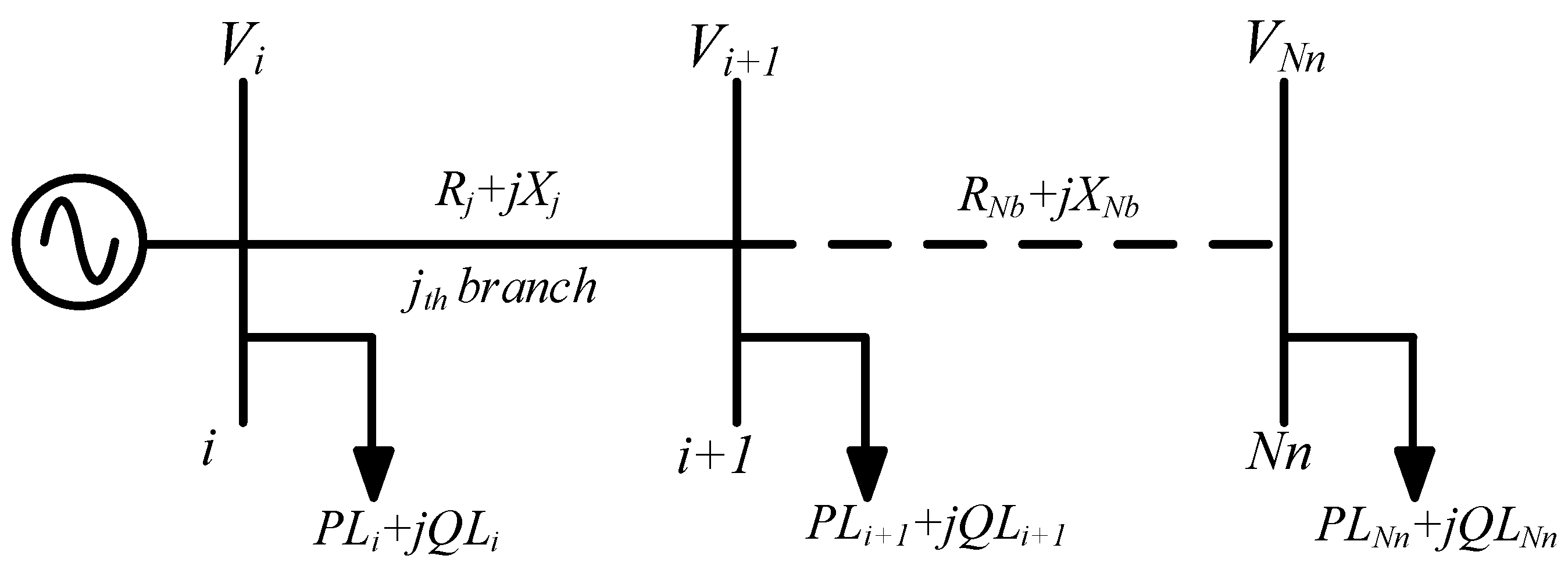
2.1. Power Flow

By applying the load flow, total power loss can be calculated from Figure 1. The voltages at nodes i and i + 1 are $V_i\angle {\delta }_i$ and $V_{i+1}\angle {\delta }_{i+1}$, respectively and given in Equations (1) and (2); where $V_i\angle {\delta }_i$ and $V_{i+1}\angle {\delta }_{i+1}$ are the sending end and the receiving end node voltages. The current I_j from node i to node i+1 is given in Equation (3), and the Total Active Power Loss (TPL); Total Reactive Power Loss (TQL); and Total Apparent Power Loss (TSL) in the system for a number of branches N_b are given in Equations (4)–(6), respectively:

$$V_{i+1}=\sqrt{\frac{V_i{}^2}{2}-\left(P{L}_{i+1}.R_j+Q{L}_{i+1}.X_j\right)+\sqrt{{\left\{\frac{V_i{}^2}{2}-\left(P{L}_{i+1}.R_j+Q{L}_{i+1}.X_j\right)\right\}}^2-\left(R_j^2+X_j^2\right)\left(P{L}_{i+1}^2+Q{L}_{i+1}^2\right)}}$$

(1)

$${\delta }_{i+1}={\delta }_i-{\tan }^{-1}\left[\frac{P_{i+1}{X}_j-Q_{i+1}{R}_j}{V_{i+1}{}^2+P_{i+1}{R}_j+Q_{i+1}{X}_j}\right]$$

(2)

$$I_j=\frac{V_i\angle {\delta }_i-V_{i+1}\angle {\delta }_{i+1}}{Z_j}$$

(3)

$$TPL={\displaystyle \sum _{j=1}^{N_b}{R}_j}{I}_j^2$$

(4)

$$TQL={\displaystyle \sum _{j=1}^{N_b}{X}_j}{I}_j^2$$

(5)

$$TSL={\displaystyle \sum _{j=1}^{N_b}{Z}_j}{I}_j^2$$

(6)

where R_j, X_j and Z_j are the resistance, reactance and impedance of jth branch, respectively; PL_i, QL_i are the active and reactive power, respectively at the node i; PL₁ = 0, QL₁ = 0, V₁ = 1, ${\delta }_1$ = 0; TPL, TQL, TSL are the total active power loss, total reactive power loss and total apparent for all N_b branches; and I_j is the total current of the active and reactive component flowing between ith and (i + 1)th buses.

2.2. Objective Function

The reconfiguration can be defined as the process of changing the status of the network switches to achieve a required aim. Loss minimization, load balancing, a maximum of minimum bus voltage, and maximum voltages up to nominal are the most frequent objective functions for network reconfiguration. In this paper, the objective function was to minimize the active power loss while overcoming the operational limitations. The objective function applied to find the minimum value of total power loss is shown in Equation (7).

$$f(x)=min TPL$$

(7)

x = [Tie₁; Tie₂; …; Tie_Ntie; Sw₁; Sw₂; …; Sw_NSw]

where x is the control variables vector; Tie_i is the state of the ith tie switch; and Sw_i is the switch number.

Most similar distribution network reconfiguration algorithms combine the index of TPL with the index of minimum voltage as a multi-objective optimal problem. The proposed objective is a mono-objective function; therefore, this design is more reasonable. According to the following case study, it is disclosed that the algorithm being compared with the proposed cannot achieve the minimum TPL due to the compromise with the index voltage. In fact, pursuing a voltage that is as high as possible in range is unreasonable. The reason lies in the fact that the utility has provided qualified power to the customer by means of the allowable voltage range limitation. Thus, the utility needs to pursue its maximum profit, that is, the single minimum TPL should be an appropriate goal. As for the power quality, different from the minimum voltage, an index of average voltage should replace it, which should be a reasonable index to evaluate the power quality from the viewpoint of utility and customers, which should be designed as follows.

2.3. Constraints

In any network reconfiguration, the power flow analysis can be achieved by calculating the bus voltage, branch current and power loss of a network of every branch. The requirements of the objective function:

• Bus voltage ought to be inside the upper and lower limits as shown in Equation (8).

  $$V_{i,\min }\le \left|V_i\right|\le V_{i,\max };i=1,2,\dots .N_n$$

  (8)

  where V_i,min and V_i,max are the minimum and maximum voltage boundaries of bus i; N_b represents the total number of branches.
• Branch current magnitudes should not exceed the designed overcurrent limitation of each branch as shown in Equation (9).

  $$\left|I_j\right|\le I_{j,\max };j=1,2,\dots .N_b$$

  (9)

  where I_j,max is the current upper limit of branch j; N_n represents the total number of buses in distribution network.
• Always keep the network structure as radial as shown in Equation (10).

  $$\begin{array}{ccc}\det (A)=1\hfill & or-1\hfill & radialsystem\hfill \\ \det (A)=0& & notradialsystem\hfill \end{array}$$

  (10)

  where A is the incidence bus matrix.

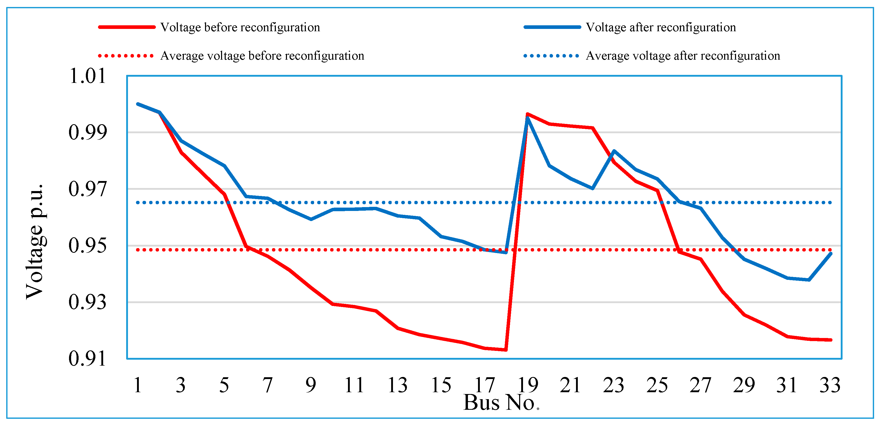
2.4. Average Voltage Concept

The V_min index is usually used in distribution network voltage studies. In network reconfiguration analysis, the V_min index is not good enough to choose the best solution because the resources of negative power compensation is inadequate to boost the V_min above 0.95, which is the code voltage. In addition, it is hard to deal with many bus voltages to decide whether or not there has been a voltage improvement in the distribution network as voltage improvement may have taken place in some buses and not in others, or may have even become worse in some buses. In this paper, a new index of average voltage is proposed to manage all buses voltages and satisfy most of the electrical utility constraints. The index is given in Equation (11).

$$V_{av}=\frac{{\displaystyle \sum _{i=1}^{N_n}{V}_i}}{N_n}$$

(11)

where V_av is the average voltage of the system; V_i is the voltages at bus i; N_n is the number of network buses.

3. Reconfiguration Method

Network reconfiguration is a method of changing the topological regulation of the distribution network’s feeders by changing the state of switches (designed for both security and configuration managing) with an operating system guarantee of satisfying the constraints [13]. Therefore, the switching operation for branch exchange is the basic control action in network reconfiguration [1]. For a large network, the difficulty of network reconfiguration is finding in the status (open or closed) the optimal configuration and the ability to handle switches to assure sections of the network. The primary aim of network reconfiguration is to determine the topology in which the active power loss is minimized to be as low as possible [14]. To reach optimal configuration, any proposed algorithm for optimization should be run a few times with a different random parameter set each time [15], where the random values of the parameters may give better or worse results to the reference objective [16]. The switches set are chosen based on the enhancement in the objective function. In the MPSO algorithm, particles move to be close to the best position and find the global minimum point [17]. The worse result is neglected while the better one is stored and recorded as the optimal result unless a better one is obtained, and is represented by Pbest_i. Thus far, the best global position of the swarm initiate is indicated by Gbest_i.

The particle swarm optimization (PSO) was first proposed by Eberhart and Kennedy [17]. The PSO algorithm was developed as an optimization technique, and was inspired by the collective behavior of free animals. The PSO has been broadly recognized as a global optimization algorithm, and is a population-based, self-versatile, stochastic optimization method [18]. The mathematical modeling and simulation swarm of birds look for food (particles) [19] and the particles move around the multi-dimension look space until they locate the ideal result. Based on the discussion above, the velocity equation for the PSO is as follows:

$$v_{ij}{}^{k+1}=w^{old}{v}_{ij}{}^k+c_1^{old}{r}_1(Pbes{t}_{ij}{}^k-S_{ij}{}^k)+c_2^{old}{r}_2(Gbes{t}_i{}^k-S_{ij}{}^k)$$

(12)

where old inertia weight w^old = constant; old learning factors $c_1^{old}$ = constant; $c_2^{old}$ = constant.

The equations for the MPSO is as follows:

-

Velocity upgrading of each particle per Equation (13)

$$v_{ij}{}^{k+1}=w^{new}{v}_{ij}{}^k+c_1^{new}{r}_1(Pbes{t}_{ij}{}^k-S_{ij}{}^k)+c_2^{new}{r}_2(Gbes{t}_i{}^k-S_{ij}{}^k)$$

(13)

i = 1, 2, …, N_D, j = 1, 2,…, N_par

-

Position updating according to Equation (14)

$$S_{ij}{}^{k+1}=S_{ij}{}^k+v_{ij}{}^{k+1}$$

(14)

-

Inertia weight updating according to Equation (15)

$$w^{new}=w_{max}-\frac{\left(w_{max}-w_{min}\right). k}{k_{max}}$$

(15)

$$c_1^{new}=Rand()$$

(16)

$$c_2^{new}=Rand()$$

(17)

The implementation of the network reconfiguration in real-time simulation required fast evaluation of the configuration. In addition, in distribution system automation, fast optimization is required to manage configuration issues. Therefore, in this paper, the inertia weight is modified to w^new, according to Equation (15) to enhance the speed control performance of the previous record of velocities on the present velocity. Gradually, during the simulation, the value of w^new decreases linearly from w_max to w_min by increasing the iteration k. $c_1^{new}$, $c_2^{new}$ given in Equations (16) and (17), which are the new learning factors of the stochastic acceleration terms coefficients. The old learning factors are modified to a random value between [0, 1] instated of constant values. This randomly increases the probability of the PSO algorithm to reach the optimal solution faster than the constant values.

where k is the iteration count; k_max is the maximum iteration; v_ij^k+1 is dimension i of the velocity of particle j at iteration k; S_ij^k+1 is dimension i of the position of particle j at iteration k; w^new is the inertia weight; w_max is maximum inertia; w_min is minimum inertia; Pbest_ij^k is dimension i of the own best position of particle j until iteration k; Gbest_ij^k is dimension i of the best particle in the swarm at iteration k; N_D dimension of the optimization issue; N_par number of particles in the swarm; and r₁, r₂ are the irregular quality created between [0, 1].

The algorithm of the MPSO is written below in Algo1.

Algo1

Step 1: Start.

Step 2: Set initial (generation of the swarm, velocity, Pbest matrix, random Gbest, wmax and wmin).

Step 3: Read system data and perform load flow.

Step 4: Set maximum iterations = iter.

Step 5: Calculate fitness function for Pbest.

Step 6: Iter = iter − 1.

Step 7: Update (velocity using Equation (13), position using Equation (14) and weight coefficient using Equation (15)).

Step 8: Calculate fitness function for each particle.

Step 9: If not satisfying all constraints in Equations (8)–(10) then go to Step 6; otherwise go to Step 10.

Step 10: If particle fitness > Pbest fitness then go to Step 6; otherwise go to Step 11.

Step 11: Pbest fitness = particle fitness.

Step 12: If iter = 0 then go to Step 13; otherwise go to Step 6.

Step 13: Print the results (switches sets, TPL, TQL, TSL, Vav, Vmin).

Step14: Stop.

3.1. MPSO Parameters

The parameters of the PSO and MPSO algorithms for the standard 33-bus network are given in

Table 1. Particle swarm optimization (PSO) and modified particle swarm optimization (MPSO) parameters.

No.	Parameters	PSO Values	MPSO Values
1	No. of birds (Npar)	20	20
2	Maximum number of bird steps	100	100
3	$c_1^{old}$, $c_2^{old}$	1.2, 0.12	-
4	$c_1^{new}$, $c_2^{new}$	-	Rand, Rand
5	wold	0.8	-
6	wmax, wmin	-	1, 0.05
7	Dimensions (ND)	5	5
8	$r_1$, $r_2$	Rand, Rand	Rand, Rand

.

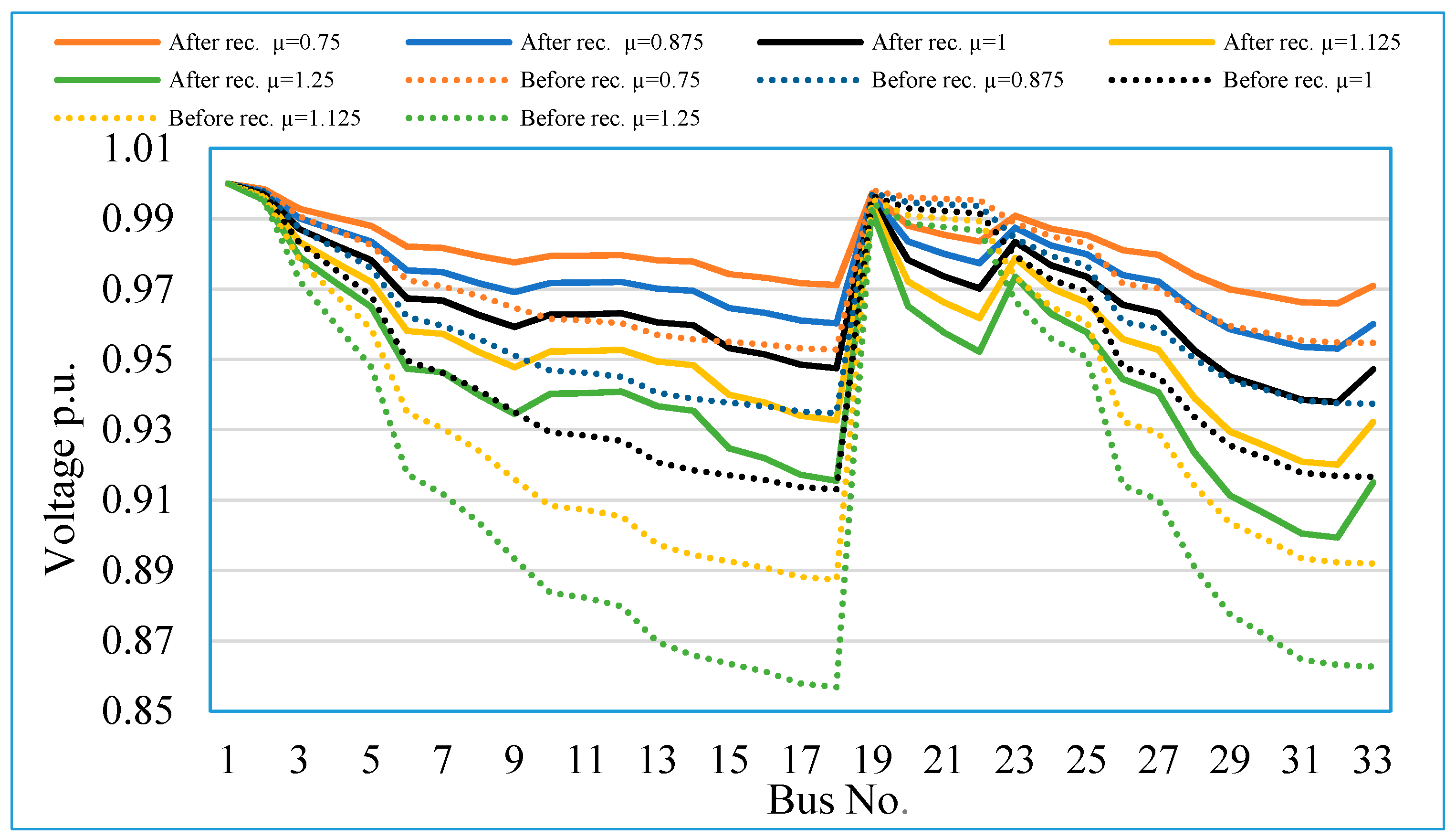
3.2. Load Demand Variation

3.2.1. Case 1

The load demands (active and reactive) in the buses are changed linearly from the light load (µ = 0.75) up to the peak (µ = 1.25) load demand with a step change of 12.5%. In each load demand level, the status of opened switches, total active power loss, total reactive power loss, total apparent power loss, average voltage and minimum voltage are calculated under different configurations. Where the proposed approach supports the operators in distribution systems to select the best configuration that provides minimum power loss under the changes in load demand level by µ. The load demand varies as in Equations (18) and (19).

$$P{L}_i=\mu P{L}_{i0}$$

(18)

$$Q{L}_i=\mu Q{L}_{i0}$$

(19)

where µ represents the value of the load variation ratio; and PL_i0 and QL_i0 represent the reference constant active and reactive power of the ith load.

The algorithm of Case 1 is written below in Algo2.

Algo2

Step 1: Start.

Step 2: Read line and load data of the test network.

Step 3: Compute the new PLi and QLi using Equations (18) and (19).

Step 4: Read the tie-lines configuration set.

Step 5: Perform load flow on new load demand (active and reactive).

Step 6: Print the results (switches sets, TPL, TQL, TSL, Vav, Vmin).

Step 7: Repeat steps 4–6 and find the results based on the different configurations.

Step 8: Find the optimal switches set based on the objective function.

Step 9: Repeat steps 2–8 and find the results based on the different ratio µ.

Step 10: Stop.

3.2.2. Case 2

Modern power systems are a complex mixture of static and dynamic elements, working in different configurations [20]. A constant load model that represents the power relationship to voltage magnitude and frequency can be defined as a polynomial load [21]. The general form of a load model, consisting of real and reactive power dependences on voltage (V) and frequency (f), is as shown in Equations (20) and (21).

$$P{L}_i=f_{PL}(V,f)$$

(20)

$$Q{L}_i=f_{QL}(V,f)$$

(21)

where (PL_i) and (QL_i) are the active and reactive load demand; f_PL, f_QL are the functions of active and reactive load demand of the system.

A load dependence on frequency is often neglected since voltage changes are much more frequent and more noticeable than the changes in system frequency [22]. In this work, the frequency is kept constant by the main grid connection; therefore, Equations (22) and (23) represent the load model depending on the changes in bus voltages. Demands were changed to be voltage-dependent, and network reconfiguration was modified to the voltage profile of the network buses. Therefore, demand behavior changed with the network reconfiguration. To perform the actual active and reactive load, the load was represented as voltage-dependent as given in Equations (22) and (23).

$$P{L}_i=P{L}_{i0}\left[p_1{\left(\frac{V_i}{V_{i0}}\right)}^2+p_2{\left(\frac{V_i}{V_{i0}}\right)}^1+p_3{\left(\frac{V_i}{V_{i0}}\right)}^0\right]$$

(22)

$$Q{L}_i=Q{L}_{i0}\left[q_1{\left(\frac{V_i}{V_{i0}}\right)}^2+q_2{\left(\frac{V_i}{V_{i0}}\right)}^1+q_3{\left(\frac{V_i}{V_{i0}}\right)}^0\right]$$

(23)

$$p_1+p_2+p_3=1$$

(24)

$$q_1+q_2+q_3=1.$$

(25)

Additionally, Equations (22) and (23) represent a ZIP model, where Z, I, and P represent the load components of constant impedance, constant current, and constant power, respectively. The parameters (p₁ and q₁), (p₂ and q₂), and (p₃ and q₃) in Equations (24) and (25) represent the relative participation of constant impedance load, the constant current load, and the constant power for the active and reactive loads, respectively. PL_i0 and QL_i0 are the references active and reactive power of the ith consumer at rated voltage V_i0 = 1 per unit. V_i is the per unit supplying voltage of the ith consumer.

Equations (22) and (23) can be rewritten as Equations (26) and (27), respectively, for the voltage-exponential load.

$$P{L}_i=P{L}_{i0}{\left[\frac{V_i}{V_{i0}}\right]}^{\alpha }$$

(26)

$$Q{L}_i=Q{L}_{i0}{\left[\frac{V_i}{V_{i0}}\right]}^{\beta }$$

(27)

where

$$\alpha \cong \frac{p_1\times 2+p_2\times 1+p_3\times 0}{p_1+p_2+p_3}$$

(28)

$$\beta \cong \frac{q_1\times 2+q_2\times 1+q_3\times 0}{q_1+q_2+q_3}$$

(29)

α and β in Equations (26) and (27) represent the voltage-exponents characteristics of active (PL_i) and reactive (QL_i) load demand, respectively; α and β can be calculated in Equations (28) and (29), respectively. The values of the active and reactive power exponents used in this work are shown in

Table 2. Load types and exponent values [23].

Load Type	Condition	α	β
Residential Consumer	Spring and Summer/Day	0.72	2.96
	Spring and Summer/Night	0.92	4.04
	Autumn and Winter/Day	1.04	4.19
	Autumn and Winter/Night	1.30	4.38
Commercial Consumer	Spring and Summer/Day	1.25	3.50
	Spring and Summer/Night	0.99	3.95
	Autumn and Winter/Day	1.50	3.15
	Autumn and Winter/Night	1.51	3.40

.

The algorithm of Case 2 is written below in Algo3.

Algo3

Step 1: Start.

Step 2: Read line data and system data (including PLi0 and QLi0), α and β.

Step 3: Set Vi0 = 1.

Step 4: Read the tie-lines configuration set.

Step 5: Perform load flow and calculate Vi.

Step 6: Compute active and reactive power demand (PLi0 and QLi0).

Step 7: Compute the new PLi and QLi using Equations (26) and (27).

Step 8: Perform load flow based on new PLi and QLi.

Step 9: Print the results (switches sets, TPL, TQL, TSL, Vav, Vmin).

Step 10: Repeat steps 4–9 and find the results based on the different configurations.

Step 11: Find the optimal switches set based on the objective function.

Step 12: Repeat steps 2–11 and find the results based different α and β.

Step 13: Stop.

3.2.3. Case 3

DGs are an alternative technique for loss minimization in distribution networks. Few types of research have been done on reconfiguration in parallel with the DG placement [24]. In this case, multiple DGs were taken (calculated by other researchers) to analyze and demonstrate the proposed approach on the active network by applying both Algo2 and Algo3 separately to the test network.

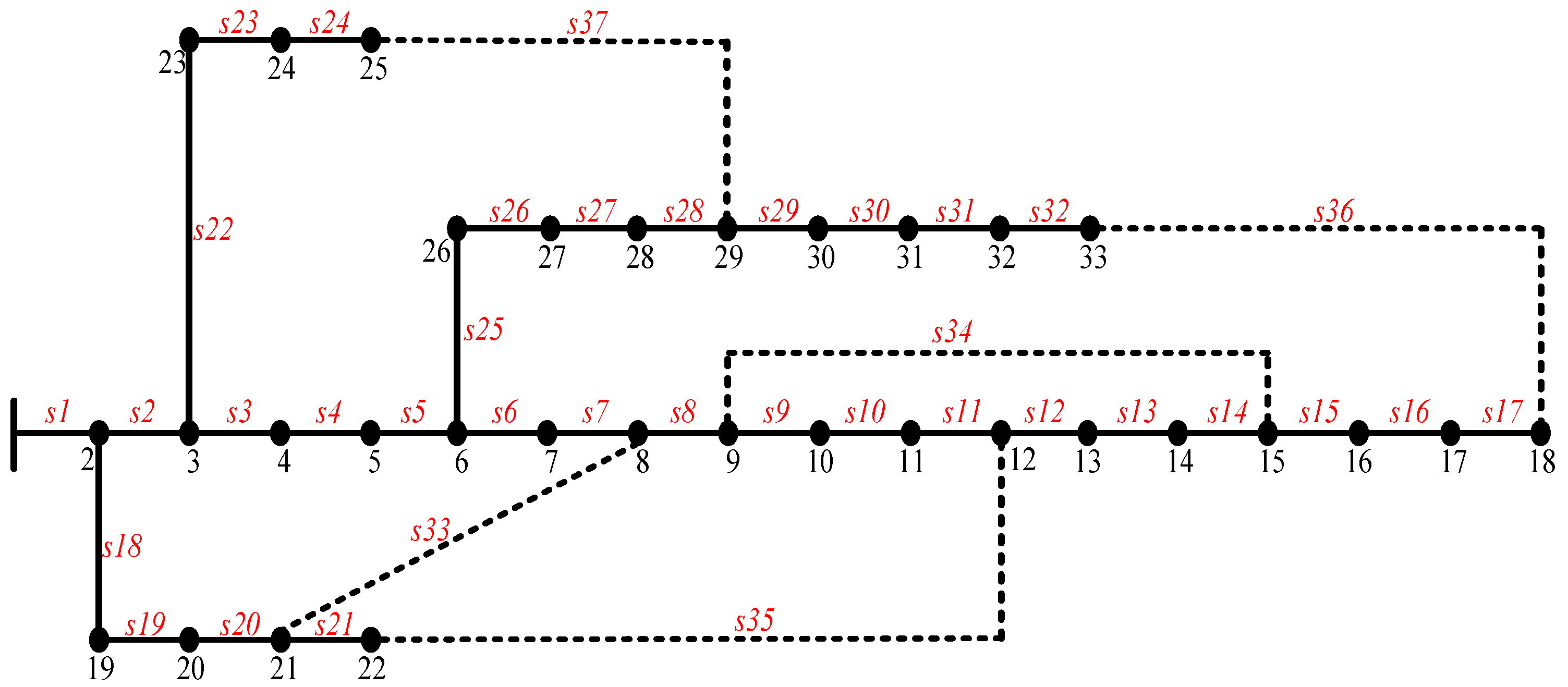
4. Case Study

In order to achieve the effectiveness of the proposed method, the operating example was set on a medium voltage distribution network. The standard 33-bus as medium scale distribution network was used here, whose base topology is shown in Figure 2. It is exceedingly used as a test example in solving network reconfiguration problems to estimate the efficiency of the proposed approach for minimizing the active power loss in distribution networks.

The sectionalizing and tie switches were put as examination switches for the reconfiguration issue. Where the N_n = 33 number of buses and N_b = 37 number of branches including 32 branches, which are usually closed switches with five redundant branches normally being open switches. The closed switches that represent the 32 branches were from s1 to s32, the opened switches that represent the tie switches were (s33, s34, s35, s36, s37) and are illustrated by the dotted lines in Figure 2. The applied test system operated at the nominal voltage of 12.66 kV. The bus number 1 represented the substation, where the voltage was considered as 1 (p.u.). The minimum voltage V_min = 0.9 (p.u.) and maximum voltage V_max = 1 (p.u.) were set as voltage constraint ranges. The line and load data of the standard 33-bus system are given in Reference [13]. The total general active and reactive loads in the network were 3615 kW and 2300 kVar, respectively. By applying the load flow in the test network, it was noticed that the total active power loss of the test network was 202.67 kW, the total reactive power loss was 135.14 kVar, and the total apparent loss was 243.60 kVA. The active power loss was equivalent to 5.45% of the active power of the loads fed by the network, and the test network had an average voltage of V_av = 0.9485 (p.u.), a minimum voltage of V₁₈ = 0.9131 (p.u.) and a maximum voltage drop by 8.69% on bus 18.

5. Results and Discussion

Network reconfiguration based on constant load demand for the standard 33-bus test network is implemented for both the conventional PSO and the MPSO. Figure 3 shows that both the PSO and MPSO reached optimal power loss (139.55 kW); PSO reaches the optimal solution after 71 iterations, while MPSO reaches the optimal solution after only 31 iterations. Therefore, the proposed MPSO is faster than the conventional PSO by 230%.

Table 3. Results of the 33-bus with different methods at constant load demands (α = 0, β = 0), µ = 1.

Methods	Open Switches	TPL (kW)	TQL (kVar)	TSL (kVA)	Vav (p.u.)	Vmin (p.u.)
Initial	s33, s34, s35, s36, s37	202.67	135.14	243.60	0.9485	0.9092
Proposed method	s07, s09, s14, s32, s37	139.55	102.30	173.03	0.9652	0.9378
FWA [2]	s07, s09, s14, s28, s32	139.98	104.88	174.91	0.9674	0.9413
MBFOA [8]	s07, s09, s14, s28, s36	141.91	105.03	176.55	0.9678	0.9378
ITS [13]	s07, s09, s14, s36, s37	142.16	102.71	175.39	0.9653	0.9336
SLR [25]	s07, s10, s14, s36, s37	142.67	103.05	176.00	0.9651	0.9336

explains the contrast between the proposed algorithm and some other algorithms mentioned in References [2,8,13,25], regarding the switches status, active power loss, reactive power loss, apparent power loss, average voltage and minimum voltage. The V_min of all the methods is just below 0.95, which means that V_min is not sufficient to be an index that is desirable, while the index of V_av is ideal for showing whole grid situations. It was noticed that the best reconfiguration of switches set was (s07, s09, s14, s32, s37) for the test network with constant feeder load demands because of its minimal apparent power loss, while V_av meets the code voltage restriction. The active power loss of the ideal reconfiguration compared with the original case, showed a reduction of active power loss by 31% from 202.67 kW to 139.55 kW with a net decrease of active power loss being 63.12 kW. The minimum voltage was improved by 2.47% from 0.9131 to 0.9378 (p.u.). The average voltage of 33 buses improved by 2% from 0.9485 to 0.9652 (p.u.). The voltage profiles of the network for the initial and optimal configuration are compared and shown in Figure 4. It can be seen that the voltage profile at all buses (except for buses 19, 20, 21, 22) were enhanced after reconfiguration.

5.1. Result of Case 1

The simulation results were compared with other algorithms which have considered reconfiguration under constant load level. There are four levels of load demand starting from µ = 0.75 to µ = 1.25 with step changes of 12.5%.

Table 4. The 33-bus network results with load factor µ = 0.75.

Methods	Open Switches	TPL (kW)	TQL (kVar)	TSL (kVA)	Vav (p.u.)	Vmin (p.u.)
Initial	s33, s34, s35, s36, s37	109.75	73.13	131.89	0.9621	0.9362
Proposed method	s07, s09, s14, s32, s37	76.61	56.16	94.99	0.9742	0.9540
FWA [2]	s07, s09, s14, s28, s32	76.87	57.58	96.05	0.9758	0.9566
MBFOA [8]	s07, s09, s14, s28, s36	77.88	57.64	96.89	0.9762	0.9540
ITS [13]	s07, s09, s14, s36, s37	77.97	56.34	96.20	0.9743	0.9510
SLR [25]	s07, s10, s14, s36, s37	78.25	56.52	96.53	0.9742	0.9510

,

Table 5. The 33-bus network results with load factor µ = 0.875.

Methods	Open Switches	TPL (kW)	TQL (kVar)	TSL (kVA)	Vav (p.u.)	Vmin (p.u.)
Initial	s33, s34, s35, s36, s37	152.20	101.45	182.92	0.9553	0.9248
Proposed method	s07, s09, s14, s32, s37	105.54	77.36	130.86	0.9698	0.9460
FWA [2]	s07, s09, s14, s28, s32	105.88	79.32	132.30	0.9716	0.9490
MBFOA [8]	s07, s09, s14, s28, s36	107.31	79.42	133.50	0.9720	0.9460
ITS [13]	s07, s09, s14, s36, s37	107.46	77.64	132.58	0.9698	0.9423
SLR [25]	s07, s10, s14, s36, s37	107.84	77.90	133.04	0.9697	0.9423

,

Table 6. The 33-bus network results with load factor µ = 1.125.

Methods	Open Switches	TPL (kW)	TQL (kVar)	TSL (kVA)	Vav (p.u.)	Vmin (p.u.)
Initial	s33, s34, s35, s36, s37	261.69	174.54	314.56	0.9414	0.9011
Proposed method	s07, s09, s14, s32, s37	178.84	131.11	221.76	0.9606	0.9295
FWA [2]	s07, s09, s14, s28, s32	179.36	134.40	224.13	0.9631	0.9335
MBFOA [8]	s07, s09, s14, s28, s36	181.91	134.63	226.31	0.9636	0.9295
ITS [13]	s07, s09, s14, s36, s37	182.29	131.70	224.89	0.9607	0.9247
SLR [25]	s07, s10, s14, s36, s37	182.95	132.14	225.69	0.9605	0.9247

and

Table 7. The 33-bus network results with load factor µ = 1.250.

Methods	Open Switches	TPL (kW)	TQL (kVar)	TSL (kVA)	Vav (p.u.)	Vmin (p.u.)
Initial	s33, s34, s35, s36, s37	329.85	220.08	396.53	0.9342	0.8889
Proposed method	s07, s09, s14, s32, s37	223.64	163.97	277.31	0.9560	0.9211
FWA [2]	s07, s09, s14, s28, s32	224.25	168.06	280.24	0.9587	0.9256
MBFOA [8]	s07, s09, s14, s28, s36	227.52	168.39	283.06	0.9593	0.9211
ITS [13]	s07, s09, s14, s36, s37	228.08	164.77	281.38	0.9561	0.9156
SLR [25]	s07, s10, s14, s36, s37	228.92	165.33	282.39	0.9558	0.9156

show the switch set (s07, s09, s14, s32, s37) had minimum active power loss compared with other methods at different load levels. Table 3 shows the results of Case 1 at µ = 1.

The voltage profile of the 33-bus network under different load steps before (with configuration set s33, s34, s35, s36, s37) and after (with configuration set s07, s09, s14, s32, s37) are shown in Figure 5. From Table 4, Table 5, Table 6 and Table 7, it is noticed that the average voltage improved by decreasing µ. The total active power loss was the minimum when µ = 0.75, and was the maximum when µ = 1.25.

5.2. Result of Case 2

Table 8. The 33-bus network results with α = 0.72, β = 2.96.

Methods	Open Switches	TPL (kW)	TQL (kVar)	TSL (kVA)	Vav (p.u.)	Vmin (p.u.)
Initial	s33, s34, s35, s36, s37	164.41	109.27	197.41	0.9557	0.9221
Proposed method	s07, s09, s14, s32, s37	120.97	88.87	150.11	0.9675	0.9432
FWA [2]	s07, s09, s14, s28, s32	121.05	91.54	151.76	0.9694	0.9459
MBFOA [8]	s07, s09, s14, s28, s36	123.05	91.21	153.17	0.9698	0.9430
ITS [13]	s07, s09, s14, s36, s37	122.26	88.57	150.97	0.9677	0.9397
SLR [25]	s07, s10, s14, s36, s37	122.71	88.86	151.50	0.9675	0.9397

,

Table 9. The 33-bus network results with α = 0.92, β = 4.04.

Methods	Open Switches	TPL (kW)	TQL (kVar)	TSL (kVA)	Vav (p.u.)	Vmin (p.u.)
Initial	s33, s34, s35, s36, s37	154.45	102.54	185.39	0.9552	0.9246
Proposed method	s07, s09, s14, s32, s37	115.72	85.07	143.62	0.9682	0.9449
FWA [2]	s07, s09, s14, s28, s32	116.94	87.75	146.20	0.9700	0.9474
MBFOA [8]	s07, s09, s14, s28, s36	117.71	87.30	146.55	0.9705	0.9446
ITS [13]	s07, s09, s14, s36, s37	116.69	84.61	144.14	0.9684	0.9416
SLR [25]	s07, s10, s14, s36, s37	117.11	84.89	144.65	0.9682	0.9416

,

Table 10. The 33-bus network results with α = 1.04, β = 4.19.

Methods	Open Switches	TPL (kW)	TQL (kVar)	TSL (kVA)	Vav (p.u.)	Vmin (p.u.)
Initial	s33, s34, s35, s36, s37	151.64	100.65	182.01	0.9556	0.9254
Proposed method	s07, s09, s14, s32, s37	114.34	84.05	141.92	0.9684	0.9453
FWA [2]	s07, s09, s14, s28, s32	115.56	86.70	144.47	0.9702	0.9477
MBFOA [8]	s07, s09, s14, s28, s36	116.28	86.24	144.77	0.9706	0.9450
ITS [13]	s07, s09, s14, s36, s37	115.26	83.58	142.37	0.9686	0.9420
SLR [25]	s07, s10, s14, s36, s37	115.67	83.85	142.87	0.9684	0.9420

,

Table 11. The 33-bus network results with α = 1.30, β = 4.38.

Methods	Open Switches	TPL (kW)	TQL (kVar)	TSL (kVA)	Vav (p.u.)	Vmin (p.u.)
Initial	s33, s34, s35, s36, s37	146.47	97.16	175.76	0.9564	0.9268
Proposed method	s07, s09, s14, s32, s37	111.86	82.20	138.81	0.9688	0.9460
FWA [2]	s07, s09, s14, s28, s32	113.02	84.77	141.28	0.9705	0.9484
MBFOA [8]	s07, s09, s14, s28, s36	113.68	84.30	141.53	0.9709	0.9457
ITS [13]	s07, s09, s14, s36, s37	112.68	81.70	139.18	0.9689	0.9428
SLR [25]	s07, s10, s14, s36, s37	113.05	81.96	139.65	0.9688	0.9428

,

Table 12. The 33-bus network results with α = 1.25, β = 3.50.

Methods	Open Switches	TPL (kW)	TQL (kVar)	TSL (kVA)	Vav (p.u.)	Vmin (p.u.)
Initial	s33, s34, s35, s36, s37	152.23	101.04	182.72	0.9555	0.9253
Proposed method	s07, s09, s14, s32, s37	115.13	84.54	142.83	0.9683	0.9449
FWA [2]	s07, s09, s14, s28, s32	116.14	87.07	145.16	0.9701	0.9474
MBFOA [8]	s07, s09, s14, s28, s36	116.96	86.69	145.59	0.9705	0.9446
ITS [13]	s07, s09, s14, s36, s37	116.16	84.16	143.44	0.9685	0.9416
SLR [25]	s07, s10, s14, s36, s37	116.56	84.41	143.92	0.9683	0.9416

,

Table 13. The 33-bus network results with α = 0.99, β = 3.95.

Methods	Open Switches	TPL (kW)	TQL (kVar)	TSL (kVA)	Vav (p.u.)	Vmin (p.u.)
Initial	s33, s34, s35, s36, s37	153.79	102.10	184.60	0.9553	0.9248
Proposed method	s07, s09, s14, s32, s37	115.50	84.89	143.34	0.9683	0.9449
FWA [2]	s07, s09, s14, s28, s32	116.68	87.54	145.87	0.9701	0.9474
MBFOA [8]	s07, s09, s14, s28, s36	117.45	87.10	146.23	0.9705	0.9446
ITS [13]	s07, s09, s14, s36, s37	116.47	84.44	143.86	0.9684	0.9416
SLR [25]	s07, s10, s14, s36, s37	116.89	84.71	144.36	0.9683	0.9416

,

Table 14. The 33-bus network results with α = 1.50, β = 3.15.

Methods	Open Switches	TPL (kW)	TQL (kVar)	TSL (kVA)	Vav (p.u.)	Vmin (p.u.)
Initial	s33, s34, s35, s36, s37	150.52	99.88	180.64	0.9557	0.9258
Proposed method	s07, s09, s14, s32, s37	114.58	84.07	142.12	0.9684	0.9449
FWA [2]	s07, s09, s14, s28, s32	115.45	86.50	144.26	0.9702	0.9475
MBFOA [8]	s07, s09, s14, s28, s36	116.30	86.16	144.74	0.9706	0.9447
ITS [13]	s07, s09, s14, s36, s37	115.66	83.74	142.79	0.9685	0.9414
SLR [25]	s07, s10, s14, s36, s37	116.04	83.98	143.25	0.9684	0.9417

and

Table 15. The 33-bus network results with α = 1.51, β = 3.40.

Methods	Open Switches	TPL (kW)	TQL (kVar)	TSL (kVA)	Vav (p.u.)	Vmin (p.u.)
Initial	s33, s34, s35, s36, s37	148.81	98.72	178.58	0.9560	0.9263
Proposed method	s07, s09, s14, s32, s37	113.63	83.39	140.94	0.9685	0.9452
FWA [2]	s07, s09, s14, s28, s32	114.54	85.83	143.13	0.9703	0.9478
MBFOA [8]	s07, s09, s14, s28, s36	115.34	85.47	143.56	0.9707	0.9450
ITS [13]	s07, s09, s14, s36, s37	114.63	83.02	141.54	0.9687	0.9420
SLR [25]	s07, s10, s14, s36, s37	115.02	83.26	141.99	0.9685	0.9420

show a comparison between the reconfiguration for different methods and different load patterns (all seasons). It was noticed from these tables that the reconfiguration pattern (s07, s09, s14, s32, s37) had the minimum TPL compared to other methods and outperformed them in terms of active power loss reduction. It was also observed that both the TQL and TSL for the optimal set were the minima for Table 8, Table 9, Table 10, Table 11, Table 12, Table 13, Table 14 and Table 15. In addition, it was observed that with different configurations, there are different TPL. This variation resulted from the variation in load demand, which is one of the characteristics of practical loads.

The voltage profiles of the 33-bus network with different load patterns at normally opened switches (s33, s34, s35, s36, s37) before and after at the best optimal reconfiguration (s07, s09, s14, s32, s37) are shown in Figure 6.

5.3. Result of Case 3

In this case, multiple DGs were calculated by Reference [24] and both Algo2 and Algo3 were applied to the new network separately. Reference [24] considered the DGs placement with reconfiguration under constant load level. The amount of active power of the DGs at unity power factor were 0.5996 MW at bus 32, 0.3141 MW at bus 33 and 0.1591 MW at bus 18, with configuration set (s07, s09, s14, s28, s32). In addition, other DG sets (1.125 MW at bus 30, 0.592 MW at bus 15 and 0.526 MW at bus 12) with configuration set (s07, s09, s14, s32, s37) were taken to compare the results under different load demands which represent what may happen during the year (all seasons). The results given in

Table 16. The 33-bus network results with distributed generators (DGs) and different load levels (set s07, s09, s14, s28, s32).

Load Levels	µ	TPL (kW)	TQL (kVar)	TSL (kVA)	Vav (p.u.)	Vmin (p.u.)
Peak load level	1.250	143.66	105.03	177.96	0.9696	0.9467
Pre-peak level	1.125	111.29	81.45	137.91	0.9738	0.9542
Constant load [24]	1	83.90	61.59	104.08	0.9779	0.9612
Pre-light level	0.875	61.32	45.31	76.24	0.9820	0.9681
Light load level	0.750	43.37	32.49	54.19	0.9860	0.9749

,

Table 17. The 33-bus network results with DGs and different load levels (set s07, s09, s14, s32, s37).

Load Levels	µ	TPL (kW)	TQL (kVar)	TSL (kVA)	Vav (p.u.)	Vmin (p.u.)
Peak load level	1.250	108.01	75.70	131.89	0.9778	0.9601
Pre-peak level	1.125	84.98	59.83	103.93	0.9822	0.9680
Constant load [24]	1	66.59	47.33	81.70	0.9865	0.9758
Pre-light level	0.875	52.68	38.10	65.02	0.9907	0.9819
Light load level	0.750	43.10	32.02	53.69	0.9950	0.9852

,

Table 18. The 33-bus network results with DGs and different exponent values (set s07, s09, s14, s28, s32).

Load Type		α	β	TPL (kW)	TQL (kVar)	TSL (kVA)	Vav (p.u.)	Vmin (p.u.)
	Constant load [24]	0	0	83.90	61.59	104.08	0.9779	0.9612
Residential	Spring and Summer/Day	0.72	2.96	73.41	53.98	91.12	0.9792	0.9642
	Spring and Summer/Night	0.92	4.04	70.21	51.66	87.17	0.9796	0.9652
	Autumn and Winter/Day	1.04	4.19	69.53	51.16	86.32	0.9797	0.9654
	Autumn and Winter/Night	1.30	4.38	68.37	50.33	84.90	0.9799	0.9658
Commercial	Spring and Summer/Day	1.25	3.50	70.58	51.93	87.63	0.9797	0.9652
	Spring and Summer/Night	0.99	3.95	70.23	51.67	87.19	0.9796	0.9652
	Autumn and Winter/Day	1.50	3.15	70.76	52.07	87.85	0.9797	0.9652
	Autumn and Winter/Night	1.51	3.40	70.12	51.60	87.06	0.9798	0.9654

and

Table 19. The 33-bus network results with DGs and different exponent values (set s07, s09, s14, s32, s37).

Load Type		α	β	TPL (kW)	TQL (kVar)	TSL (kVA)	Vav (p.u.)	Vmin (p.u.)
	Constant load [21]	0	0	66.59	47.33	81.70	0.9865	0.9758
Residential	Spring and Summer/Day	0.72	2.96	61.18	43.33	75.13	0.9873	0.9778
	Spring and Summer/ Night	0.92	4.04	59.39	42.37	72.96	0.9876	0.9784
	Autumn and Winter/ Day	1.04	4.19	50.10	42.18	72.61	0.9876	0.9786
	Autumn and Winter/ Night	1.30	4.38	58.67	41.89	72.09	0.9878	0.9789
Commercial	Spring and Summer/Day	1.25	3.50	60.03	42.84	73.75	0.9876	0.9784
	Spring and Summer/ Night	0.99	3.95	59.49	42.45	73.08	0.9876	0.9784
	Autumn and Winter/ Day	1.50	3.15	60.44	43.14	74.26	0.9876	0.9784
	Autumn and Winter/ Night	1.51	3.40	60.05	42.87	73.78	0.9877	0.9786

demonstrate the effectiveness of the proposed approach for analyzing the system under different load demand conditions with multiple DG units. Additionally, the set (s07, s09, s14, s32, s37) with its mentioned DGs had minimum active power loss compared with the others under the same conditions of load variation.

6. Conclusions

This paper presented the performance analysis of distribution system under different load demands. The main contributions of this paper are highlighted as follows: Firstly, in the field of distribution network reconfiguration, the variable load modeling technique is introduced in this paper, which is presently missing in the literature of this field. Second, a suitable objective function, the minimization of the active power loss in electrical utilities, is chosen as the objective function of distribution network reconfiguration, which is more reasonable from the viewpoint of utility since the benefit of the customers has been ensured by means of the given voltage limitation. Pursuing a higher minimum voltage through sacrificing the TPL further is unfair to the utility. Third, an average voltage is proposed to replace the minimum voltage as a new index to evaluate power quality, which is a more appropriate index from the viewpoint of both sides. Fourth, in order to estimate the effect of the proposed approach, the PSO and MPSO were successfully applied to the standard 33-bus network based on constant load demand. In order to enhance the speed control performance of the previous record of velocities on the present velocity, an inertia weight is designed. It is found that the proposed MPSO is faster than the traditional PSO by 230%. Fifth, the configuration set obtained from the MPSO, with other different optimization methods under constant load demand, is taken as test switches based on variable loads, different pattern loads without and within the presence of DGs, in order to be used by distribution operators. Different values of the load variation ratio and different exponent values are used in this analysis to illustration the practical load behavior. The results were compared with other, different sets available from an investigation of articles on distribution network reconfiguration for power loss minimization. From the test results of the test network, it was observed that the proposed solution was the best optimal configuration and had the greatest minimum power loss based on different cases. Therefore, the proposed approach can provide good analysis as well as find the best set solution for optimal distribution operation under different load conditions.

References

- Kalambe, S.; Agnihotri, G. Loss minimization techniques used in distribution network: Bibliographical survey. Renew. Sustain. Energy Rev. 2014, 29, 184–200. [Google Scholar] [CrossRef]
- Mohamed Imran, A.; Kowsalya, M. A new power system reconfiguration scheme for power loss minimization and voltage profile enhancement using fireworks algorithm. Int. J. Electr. Power Energy Syst. 2014, 62, 312–322. [Google Scholar] [CrossRef]
- Niknam, T.; Azadfarsani, E.; Jabbari, M. A new hybrid evolutionary algorithm based on new fuzzy adaptive PSO and NM algorithms for distribution feeder reconfiguration. Energy Convers. Manag. 2012, 54, 7–16. [Google Scholar] [CrossRef]
- De Oliveira, L.W.; de Oliveira, E.J.; Gomes, F.V.; Silva, I.C.; Marcato, A.L.M.; Resende, P.V.C. Artificial immune systems applied to the reconfiguration of electrical power distribution networks for energy loss minimization. Int. J. Electr. Power Energy Syst. 2014, 56, 64–74. [Google Scholar] [CrossRef]
- Tomoiagă, B.; Chindriş, M.; Sumper, A.; Sudria-Andreu, A.; Villafafila-Robles, R. Pareto optimal reconfiguration of power distribution systems using a genetic algorithm based on NSGA-II. Energies 2013, 6, 1439–1455. [Google Scholar] [CrossRef]
- Shirmohammadi, D.; Hong, H.W. Reconfiguration of electric distribution networks for resistive line losses reduction. IEEE Trans. Power Deliv. 1989, 4, 1492–1498. [Google Scholar] [CrossRef]
- Sathish Kumar, K.; Jayabarathi, T. Power system reconfiguration and loss minimization for an distribution systems using bacterial foraging optimization algorithm. Int. J. Electr. Power Energy Syst. 2012, 36, 13–17. [Google Scholar] [CrossRef]
- Naveen, S.; Sathish Kumar, K.; Rajalakshmi, K. Distribution system reconfiguration for loss minimization using modified bacterial foraging optimization algorithm. Int. J. Electr. Power Energy Syst. 2015, 69, 90–97. [Google Scholar] [CrossRef]
- Gupta, N.; Swarnkar, A.; Niazi, K.R. Distribution network reconfiguration for power quality and reliability improvement using genetic Algorithms. Int. J. Electr. Power Energy Syst. 2014, 54, 664–671. [Google Scholar] [CrossRef]
- Duan, D.-L.; Ling, X.-D.; Wu, X.-Y.; Zhong, B. Reconfiguration of distribution network for loss reduction and reliability improvement based on an enhanced genetic algorithm. Int. J. Electr. Power Energy Syst. 2015, 64, 88–95. [Google Scholar] [CrossRef]
- Saffar, A.; Hooshmand, R.; Khodabakhshian, A. A new fuzzy optimal reconfiguration of distribution systems for loss reduction and load balancing using ant colony search-based algorithm. Appl. Soft Comput. 2011, 11, 4021–4028. [Google Scholar] [CrossRef]
- Carpaneto, E.; Chicco, G. Distribution system minimum loss reconfiguration in the hyper-cube ant colony optimization framework. Electr. Power Syst. Res. 2008, 78, 2037–2045. [Google Scholar] [CrossRef]
- Nguyen, T.T.; Truong, A.V. Distribution network reconfiguration for power loss minimization and voltage profile improvement using cuckoo search algorithm. Int. J. Electr. Power Energy Syst. 2015, 68, 233–242. [Google Scholar] [CrossRef]
- Salazar, H.; Gallego, R.; Romero, R. Artificial neural networks and clustering techniques applied in the reconfiguration of distribution systems. IEEE Trans. Power Deliv. 2006, 21, 1735–1742. [Google Scholar] [CrossRef]
- Fang, H.; Chen, L.; Shen, Z. Application of an improved PSO algorithm to optimal tuning of PID gains for water turbine governor. Energy Convers. Manag. 2011, 52, 1763–1770. [Google Scholar] [CrossRef]
- Cai, J.; Ma, X.; Li, Q.; Li, L.; Peng, H. A multi-objective chaotic particle swarm optimization for environmental/economic dispatch. Energy Convers. Manag. 2009, 50, 1318–1325. [Google Scholar] [CrossRef]
- Niknam, T.; Mojarrad, H.D.; Meymand, H.Z. A novel hybrid particle swarm optimization for economic dispatch with valve-point loading effects. Energy Convers. Manag. 2011, 52, 1800–1809. [Google Scholar] [CrossRef]
- Selvakumar, A.I.; Thanushkodi, K. A new particle swarm optimization solution to Nonconvex economic dispatch problems. IEEE Trans. Power Syst. 2007, 22, 42–51. [Google Scholar] [CrossRef]
- Deepa, S.N.; Sugumaran, G. Model order formulation of a multivariable discrete system using a modified particle swarm optimization approach. Swarm Evol. Comput. 2011, 1, 204–212. [Google Scholar] [CrossRef]
- Savio, A.; Bignucolo, F.; Sgarbossa, R.; Mattavelli, P.; Cerretti, A.; Turri, R. A novel measurement-based procedure for load dynamic equivalent identification. In Proceedings of the 2015 IEEE 1st International Forum on Research and Technologies for Society and Industry Leveraging a better tomorrow (RTSI), Torino, Italy, 16–18 September 2015. [Google Scholar]
- Price, W.W.; Chiang, H.-D.; Clark, H.K.; Vaahedi, E. Load representation for dynamic performance analysis (of power systems). IEEE Trans. Power Syst. 1993, 8, 472–482. [Google Scholar]
- Milanović, I.V.; Matevosiyan, J.; Borghetti, A.; Djokić, S.Z.; Dong, Z.Y. Modelling and Aggregation of Loads in Flexible Power Networks; CIGRE Technical Brochure 566; CIGRE: Paris, Frace, 2014. [Google Scholar]
- Mousavi, S.M.; Abyaneh, H.A. Effect of load models on probabilistic characterization of Aggregated load patterns. IEEE Trans. Power Syst. 2011, 26, 811–819. [Google Scholar] [CrossRef]
- Bayat, A.; Bagheri, A.; Noroozian, R. Optimal siting and sizing of distributed generation accompanied by reconfiguration of distribution networks for maximum loss reduction by using a new UVDA-based heuristic method. Int. J. Electr. Power Energy Syst. 2016, 77, 360–371. [Google Scholar] [CrossRef]
- Dall’Anese, E.; Giannakis, G.B. Sparsity-Leveraging reconfiguration of smart distribution systems. IEEE Trans. Power Deliv. 2014, 29, 1417–1426. [Google Scholar] [CrossRef]