
Orchestrating an Effective Formulation to Investigate the Impact of EMSs (Energy Management Systems) for Residential Units Prior to Installation

 , , , , and
Abstract
:1. Introduction
- have knowledge regarding the use of EMSs (awareness),
- be able to install EMS (investment) and then,
- get monetary benefits (cost savings).
1.1. Motivation
2. Related Work
2.1. Problem Statement and Contribution
3. Performance Metric for EMS: UCL
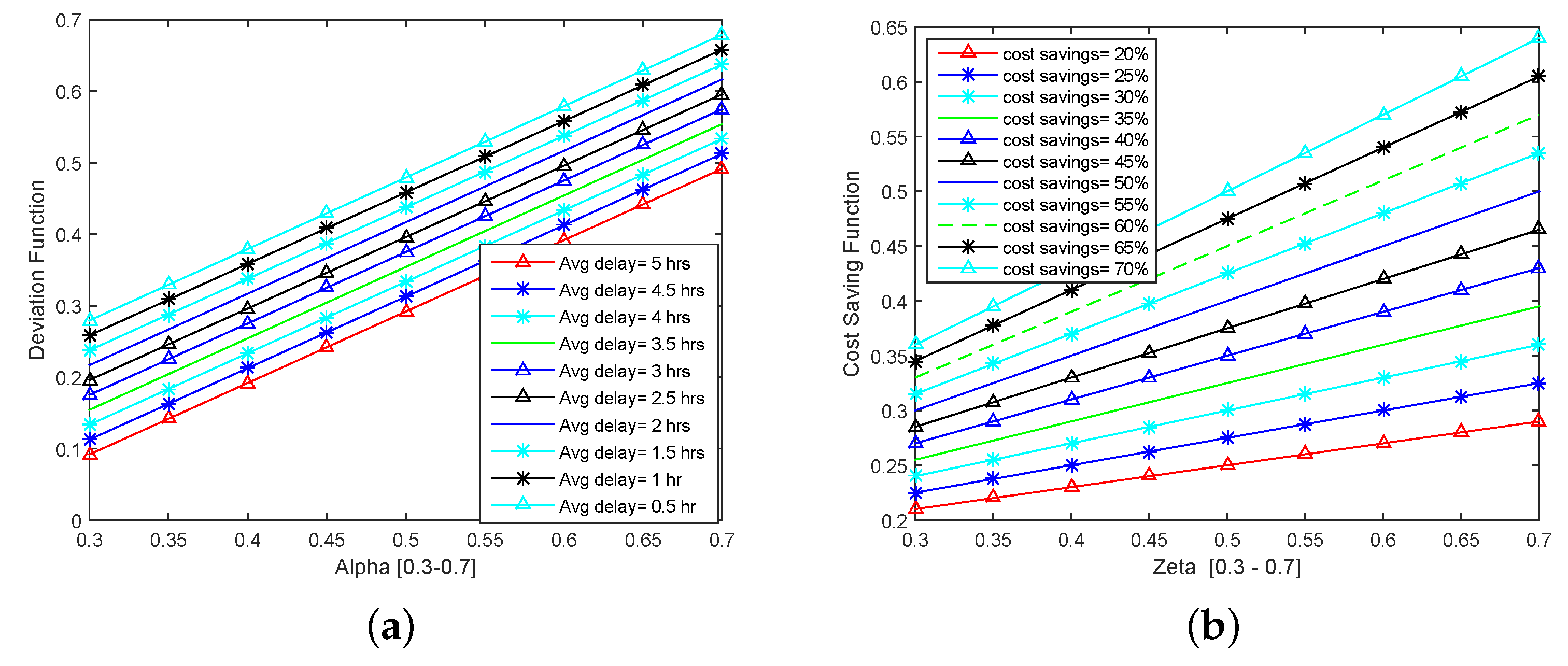
- Deviation function: appliance delay in ToU,
- Cost saving function:
- Saving function: reduction in utility bills.
- Investment function: Return On Investment (ROI) period.
3.1. User Comfort Level
3.1.1. Deviation Function
3.1.2. Cost Saving Function
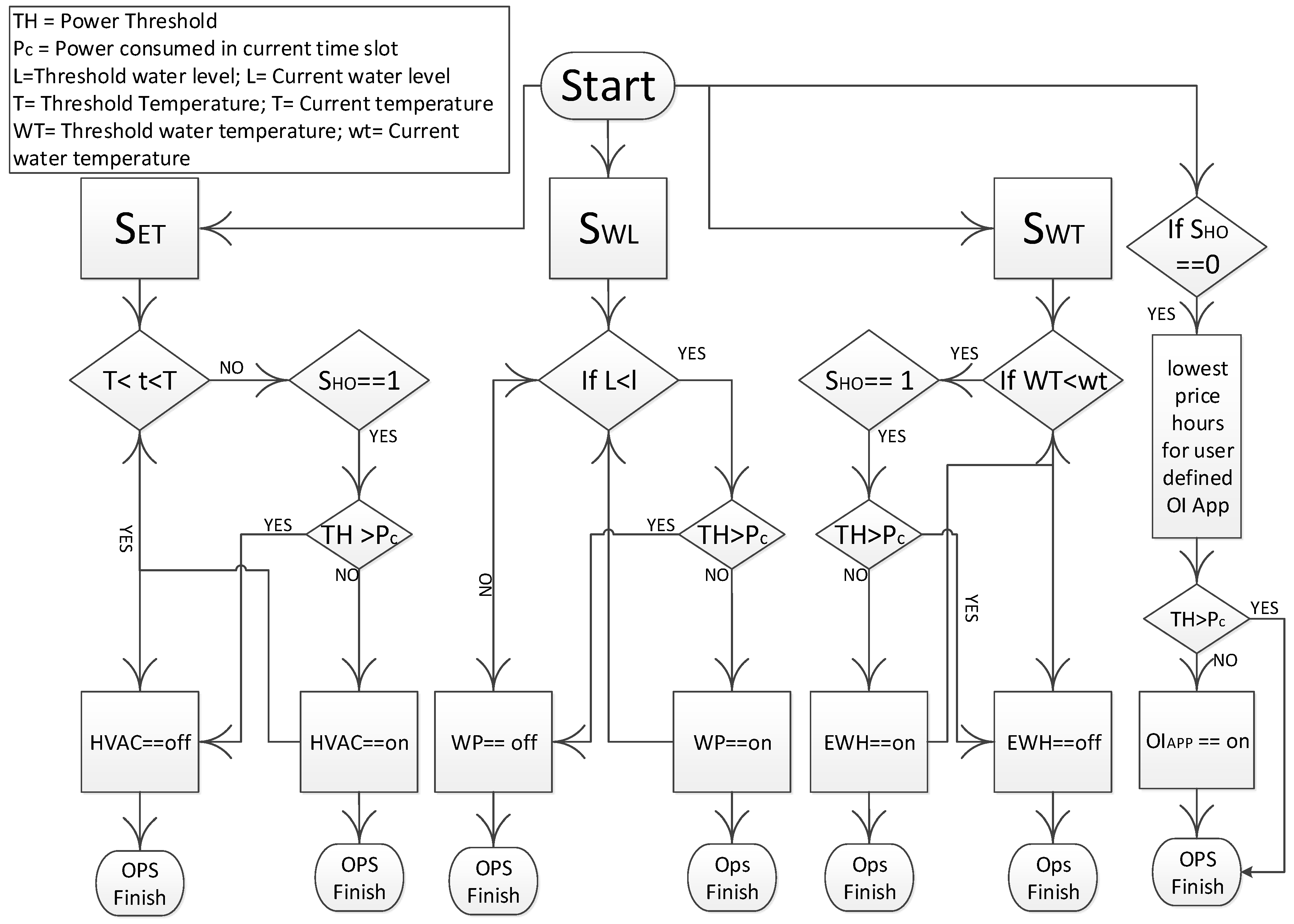
3.2. Algorithm: UCL
| Algorithm 1 Calculate . |
|
4. Basic Building Blocks: EMS
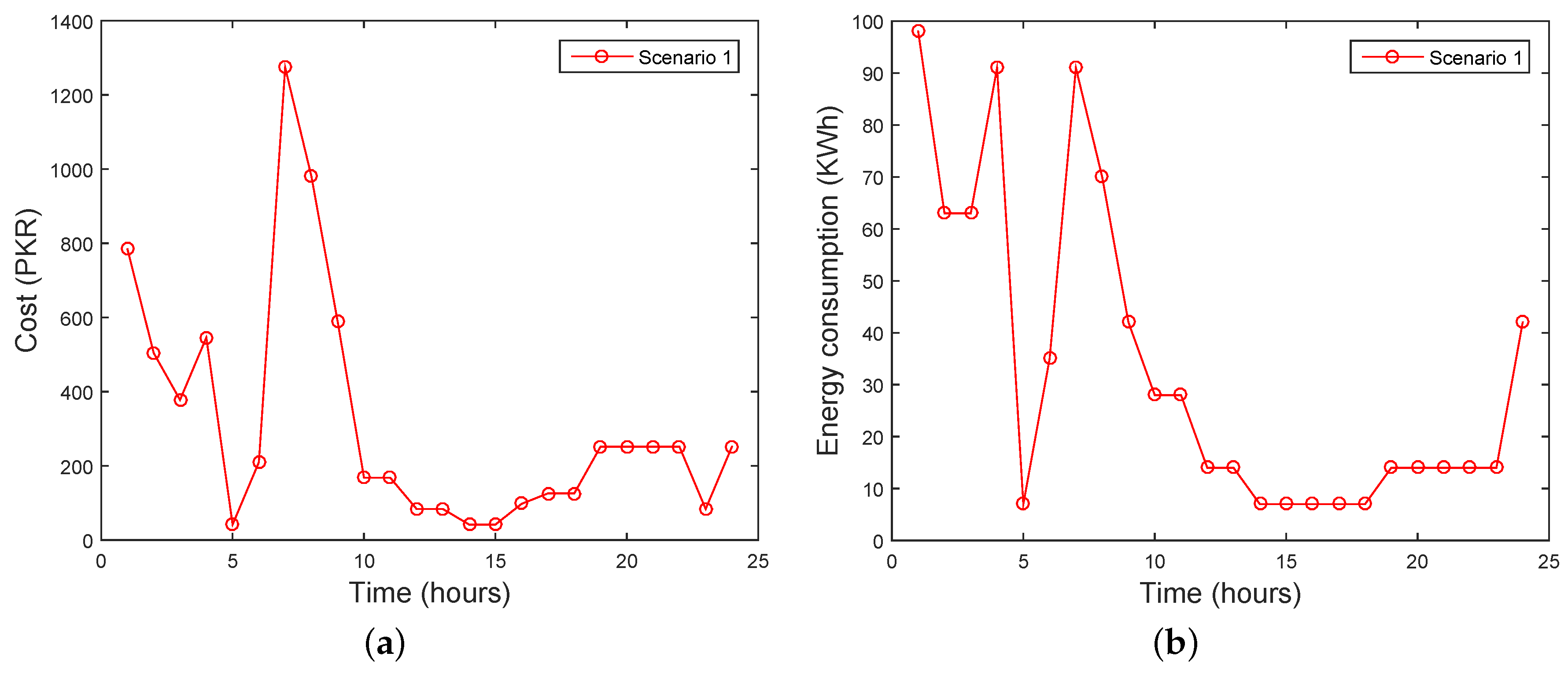
- Scenario 1: without EMS (baseline model),
- Scenario 2: EMS by using sensors,
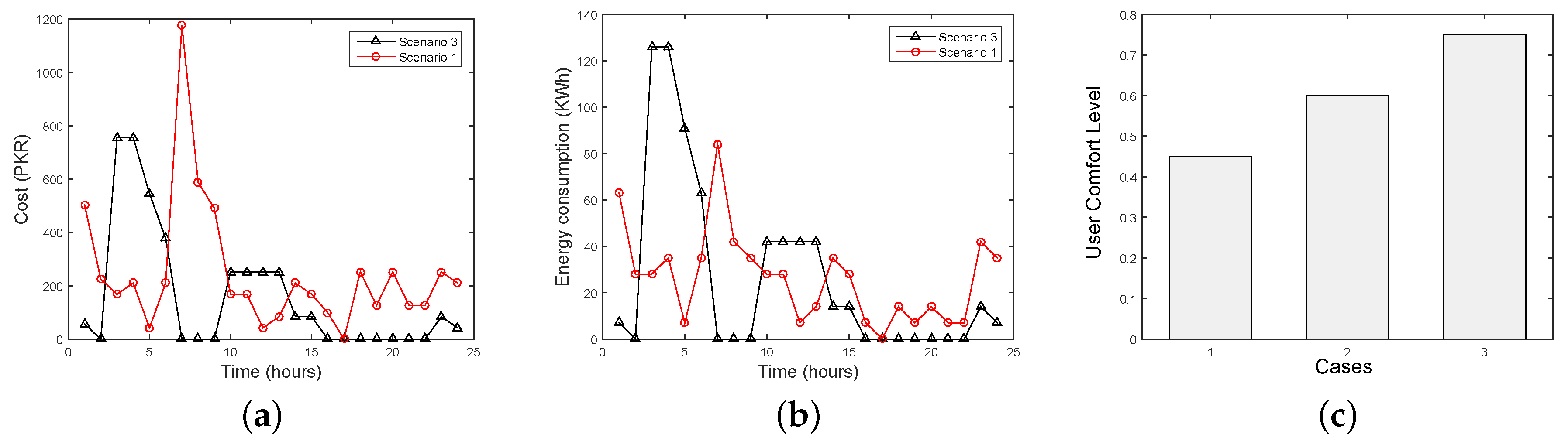
- Scenario 3: EMS by using optimization techniques,
- Scenario 4: EMS by using Scenario 2 + Scenario 3,
- Scenario 5: EMS by using storage device + Scenario 3,
- Scenario 6: EMS by using storage device + Scenario 4
4.1. Scenario 1: Without EMS
4.2. Scenario 2: EMS by Using Sensors
4.3. Scenario 3: EMS by Using Optimization Techniques
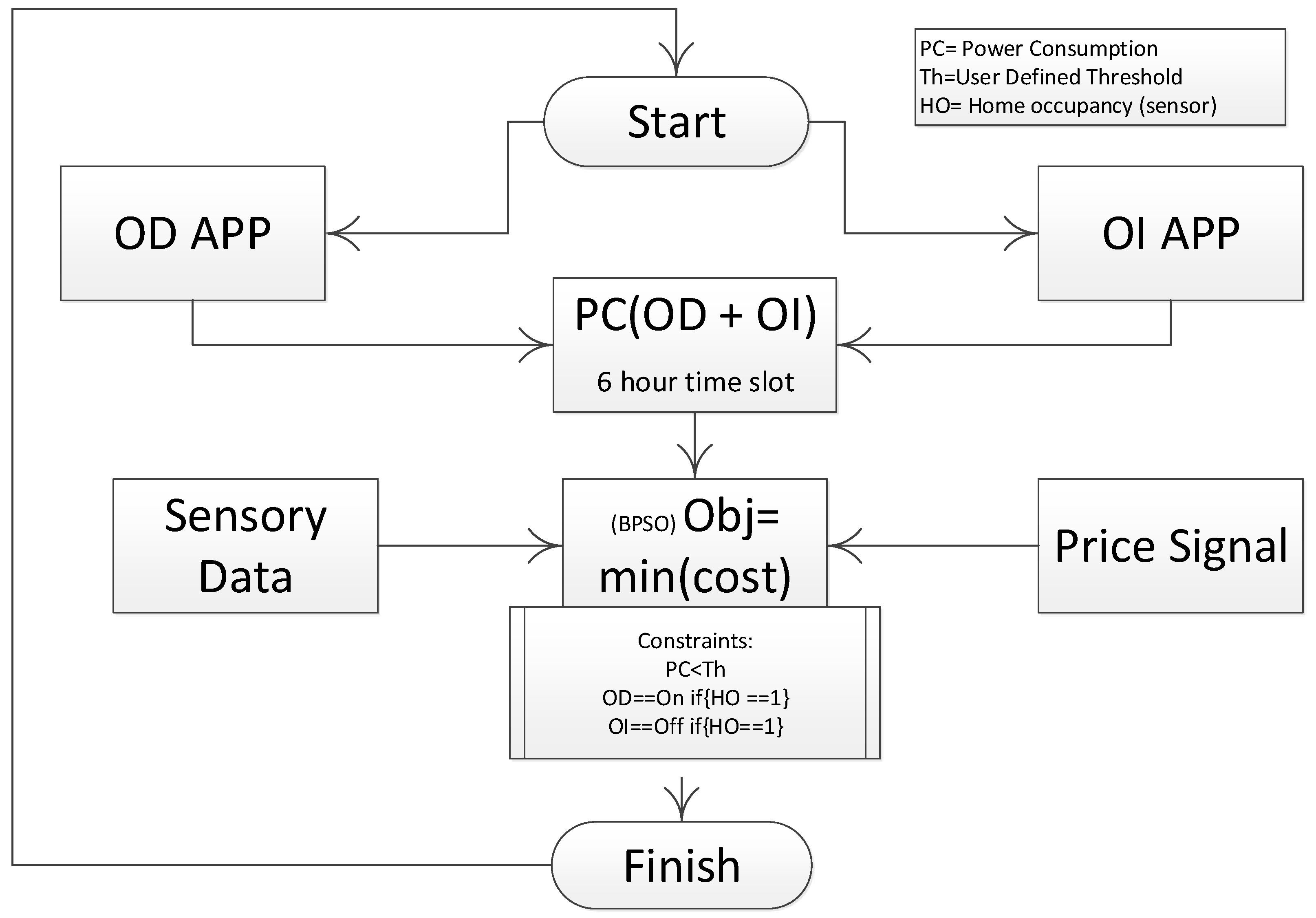
4.4. Scenario 4: EMS by Using Scenario 2 + Scenario 3
4.5. Scenario 5: EMS by Using Storage Device + Scenario 3
| Algorithm 2 Energy storage system. |
|
4.6. Scenario 6: EMS by Using Storage Device + Scenario 4
5. Results and Discussion
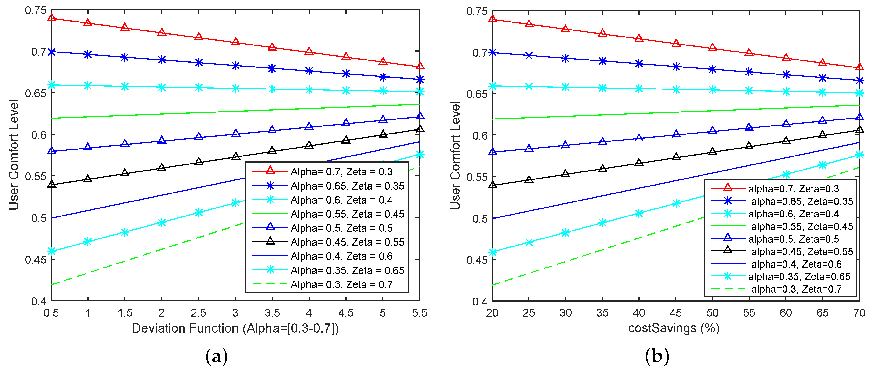
5.1. Numerical Studies: UCL
5.2. Scenario 1
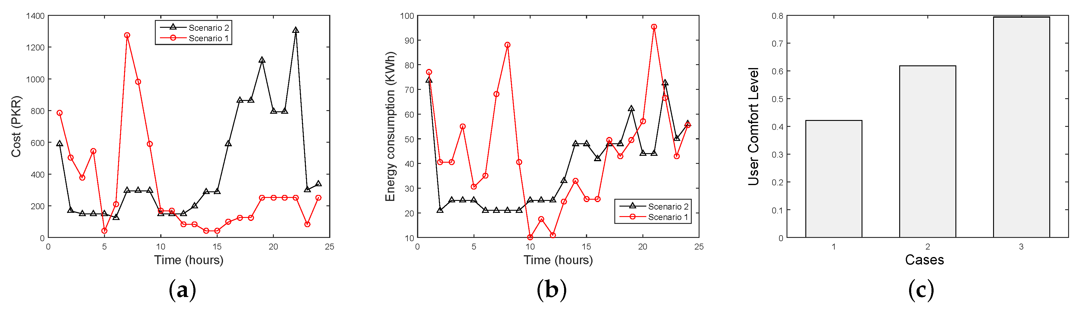
5.3. Scenario 2
5.4. Scenario 3
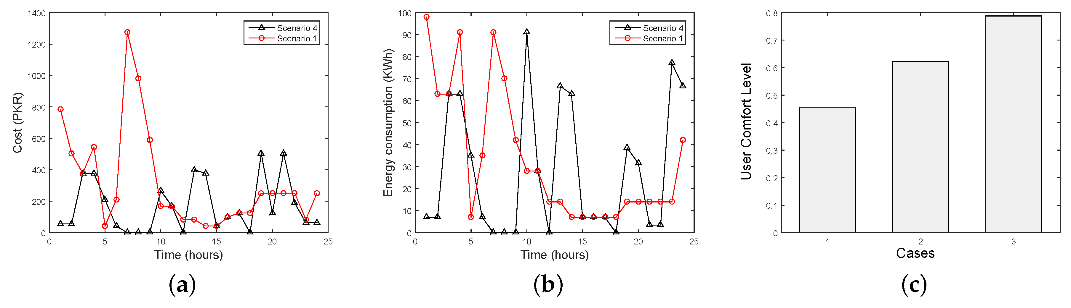
5.5. Scenario 4
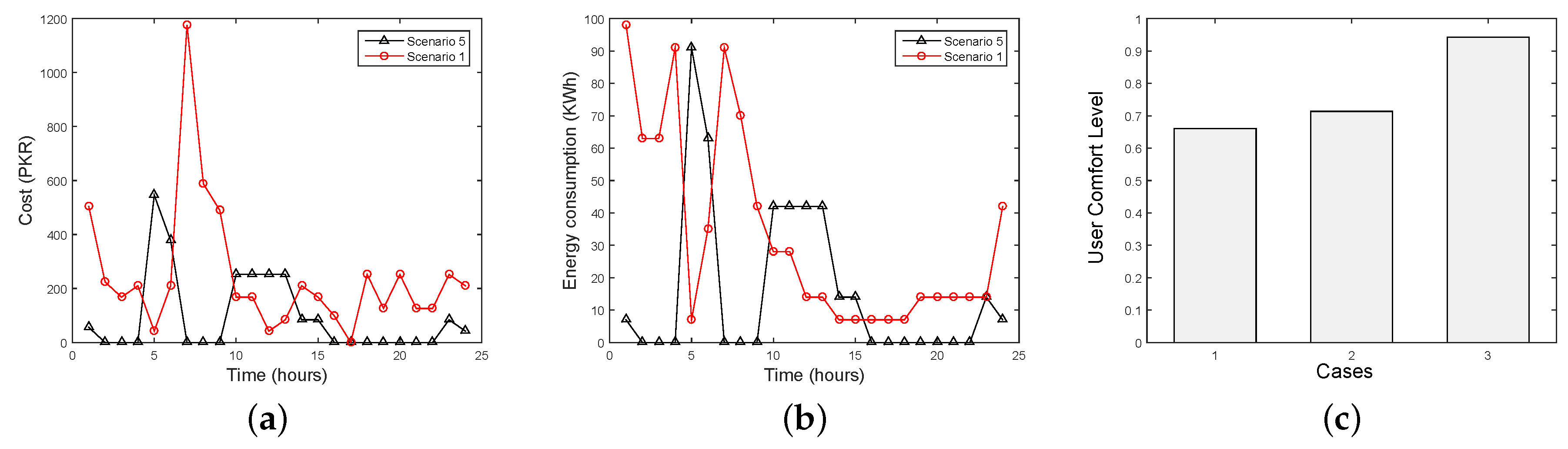
5.6. Scenario 5
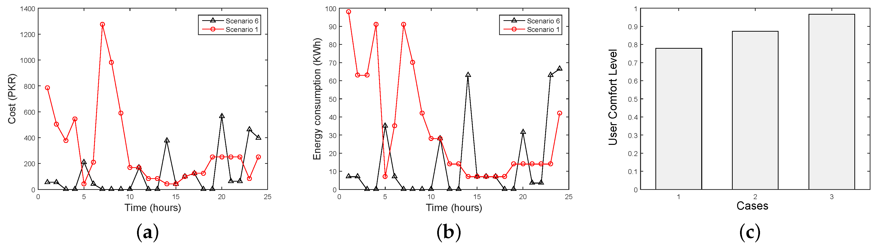
5.7. Scenario 6
6. Analysis and Policy Implications
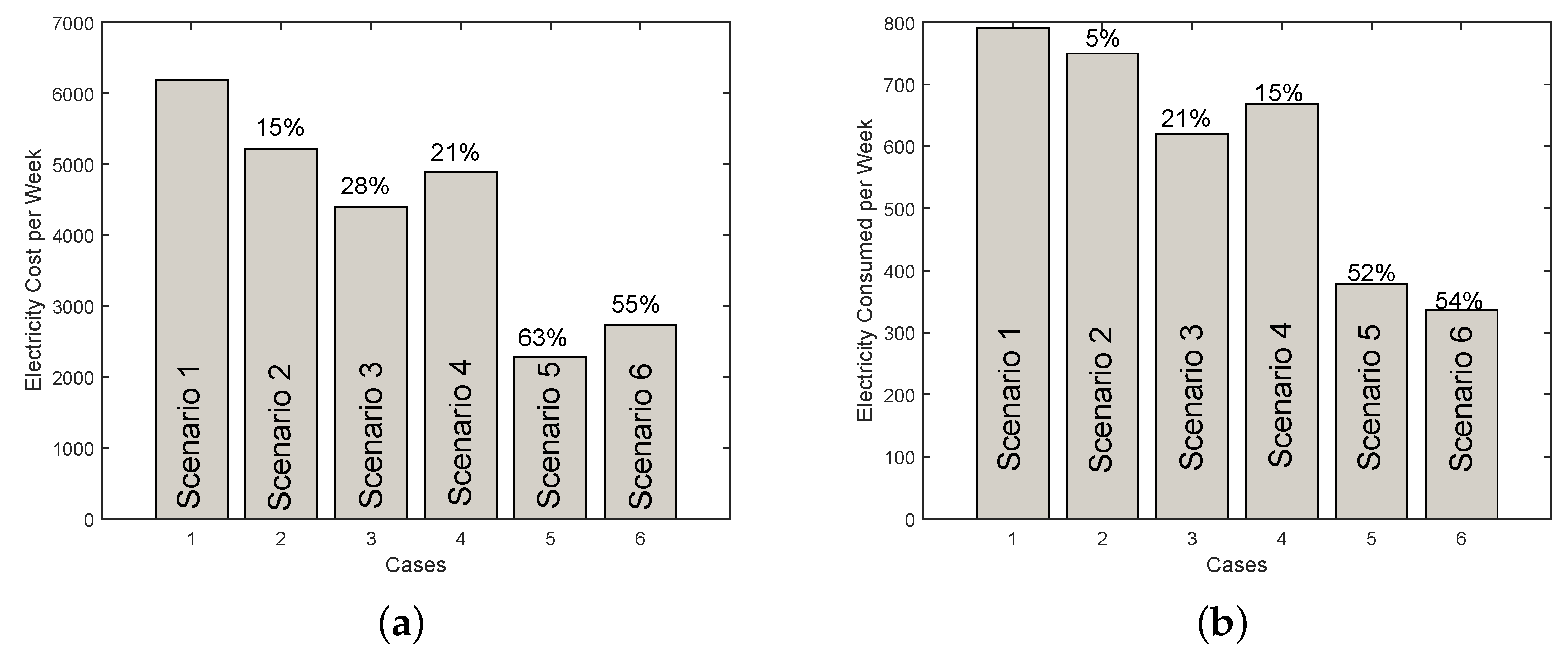
6.1. Energy and Cost Profiles
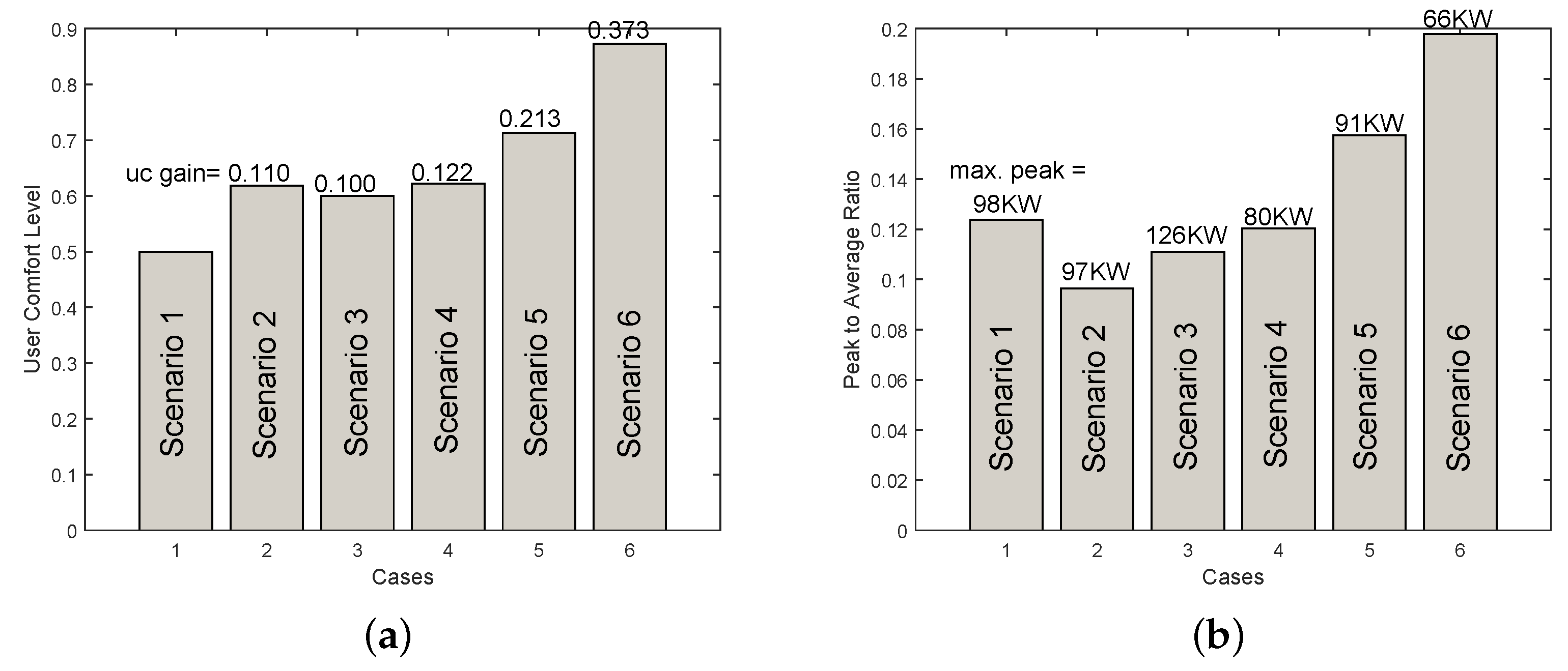
6.2. UCL and PAR Profiles
6.3. UCL Scope and Limitations
7. Conclusions
Acknowledgments
Author Contributions
Conflicts of Interest
References
- Energy Information Administration. International Energy Outlook 2016, U.S. Department of Energy. May 2016. Available online: http://www.eia.gov/outlooks/ieo/pdf/0484(2016).pdf (accessed on 7 March 2017). [Google Scholar]
- Cetin, K.S.; Tabares-Velasco, P.C.; Novoselac, A. Appliance daily energy use in new residential buildings: Use profiles and variation in time-of-use. Energy Build. 2014, 84, 716–726. [Google Scholar] [CrossRef]
- Alam, M.R.; Reaz, M.B.; Ali, M.A. A review of smart homes—Past, present, and future. IEEE Trans. Syst. Man Cybern. Part C (Appl. Rev.) 2012, 42, 1190–1203. [Google Scholar] [CrossRef]
- Abushnaf, J.; Rassau, A.; Górnisiewicz, W. Impact of dynamic energy pricing schemes on a novel multi-user home energy management system. Electr. Power Syst. Res. 2015, 125, 124–132. [Google Scholar] [CrossRef]
- Bera, S.; Gupta, P.; Misra, S. D2S: Dynamic demand scheduling in smart grid using optimal portfolio selection strategy. IEEE Trans. Smart Grid 2015, 6, 1434–1442. [Google Scholar] [CrossRef]
- Taniguchi, T.; Kawasaki, K.; Fukui, Y.; Yano, S. Automated Linear Function Submission-based Double Auction for Emergent Real-Time Pricing in a Regional Smart Grid. 2015. Available online: http://arxiv.org/abs/1503.06408v1 (accessed on 2 January 2016).
- Mahmood, A.; Javaid, N.; Khan, M.A.; Razzaq, S. An overview of load management techniques in smart grid. Int. J. Energy Res. 2015, 39, 1437–1450. [Google Scholar] [CrossRef]
- Graditi, G.; Ippolito, M.G.; Telaretti, E.; Zizzo, G. Technical and economical assessment of distributed electrochemical storages for load shifting applications: An Italian case study. Renew. Sustain. Energy Rev. 2016, 57, 515–523. [Google Scholar] [CrossRef]
- Siano, P.; Graditi, G.; Atrigna, M.; Piccolo, A. Designing and testing decision support and energy management systems for smart homes. J. Ambient Intell. Humaniz. Comput. 2013, 4, 651–661. [Google Scholar] [CrossRef]
- Zheng, M.; Meinrenken, C.J.; Lackner, K.S. Agent-based model for electricity consumption and storage to evaluate economic viability of tariff arbitrage for residential sector demand response. Appl. Energy 2014, 126, 297–306. [Google Scholar] [CrossRef]
- Graditi, G.; Ippolito, M.G.; Lamedica, R.; Piccolo, A.; Ruvio, A.; Santini, E.; Siano, P.; Zizzo, G. Innovative control logics for a rational utilization of electric loads and air-conditioning systems in a residential building. Energy Build. 2015, 102, 1–7. [Google Scholar] [CrossRef]
- Qela, B.; Mouftah, H.T. Observe, learn, and adapt (OLA)—An algorithm for energy management in smart homes using wireless sensors and artificial intelligence. IEEE Trans. Smart Grid 2012, 3, 2262–2272. [Google Scholar] [CrossRef]
- Auger, A.; Doerr, B. Theory of Randomized Search Heuristics: Foundations and Recent Developments; World Scientific: Singapore, 2011. [Google Scholar]
- Hrovatin, N.; Dolšak, N.; Zorić, J. Factors impacting investments in energy efficiency and clean technologies: Empirical evidence from Slovenian manufacturing firms. J. Clean. Prod. 2016, 127, 475–486. [Google Scholar] [CrossRef]
- Menezes, A.C.; Cripps, A.; Bouchlaghem, D.; Buswell, R. Predicted vs. actual energy performance of non-domestic buildings: Using post-occupancy evaluation data to reduce the performance gap. Appl. Energy 2012, 97, 355–364. [Google Scholar] [CrossRef]
- USGBC Research Committee. A National Green Building Research Agenda. US Green Building Council, 2007. Available online: http://www.usgbc.org/Docs/Archive/General/Docs3402.pdf (accessed on 15 March 2014).
- De Wilde, P. The gap between predicted and measured energy performance of buildings: A framework for investigation. Autom. Constr. 2014, 41, 40–49. [Google Scholar] [CrossRef]
- Kibert, C.J. Sustainable Construction: Green Building Design and Delivery; John Wiley & Sons: New York, NY, USA, 2016. [Google Scholar]
- Dwaikat, L.N.; Ali, K.N. Measuring the Actual Energy Cost Performance of Green Buildings: A Test of the Earned Value Management Approach. Energies 2016, 9, 188. [Google Scholar] [CrossRef]
- Andreadou, N.; Guardiola, M.O.; Fulli, G. Telecommunication Technologies for Smart Grid Projects with Focus on Smart Metering Applications. Energies 2016, 9, 375. [Google Scholar] [CrossRef]
- Lobaccaro, G.; Carlucci, S.; Löfström, E. A Review of Systems and Technologies for Smart Homes and Smart Grids. Energies 2016, 9, 348. [Google Scholar] [CrossRef]
- Thomas, B.L.; Cook, D.J. Activity-Aware Energy-Efficient Automation of Smart Buildings. Energies 2016, 9, 624. [Google Scholar] [CrossRef]
- Kan, E.M.; Kan, S.L.; Ling, N.H.; Soh, Y.; Lai, M. Multi-zone Building Control System for Energy and Comfort Management. In Hybrid Intelligent Systems; Springer: Berlin, Germany, 2016; pp. 41–51. [Google Scholar]
- Cetin, K.S.; Manuel, L.; Novoselac, A. Thermal comfort evaluation for mechanically conditioned buildings using response surfaces in an uncertainty analysis framework. Sci. Technol. Built Environ. 2016, 22, 140–152. [Google Scholar] [CrossRef]
- Mendes, T.D.; Godina, R.; Rodrigues, E.M.; Matias, J.C.; Catalão, J.P. Smart home communication technologies and applications: Wireless protocol assessment for home area network resources. Energies 2015, 8, 7279–7311. [Google Scholar] [CrossRef]
- Ikpehai, A.; Adebisi, B.; Rabie, K.M.; Haggar, R.; Baker, M. Experimental Study of 6LoPLC for Home Energy Management Systems. Energies 2016, 9, 1046. [Google Scholar] [CrossRef]
- Faria, P.; Vale, Z.; Baptista, J. Constrained consumption shifting management in the distributed energy resources scheduling considering demand response. Energy Convers. Manag. 2015, 93, 309–320. [Google Scholar] [CrossRef]
- Pallonetto, F.; Oxizidis, S.; Milano, F.; Finn, D. The effect of time-of-use tariffs on the demand response flexibility of an all-electric smart-grid-ready dwelling. Energy Build. 2016, 128, 56–67. [Google Scholar] [CrossRef]
- Castillo-Cagigal, M.; Matallanas, E.; Gutiérrez, A.; Monasterio-Huelin, F.; Caamaño-Martín, E.; Masa-Bote, D.; Jiménez-Leube, J. Heterogeneous collaborative sensor network for electrical management of an automated house with PV energy. Sensors 2011, 11, 11544–11559. [Google Scholar] [CrossRef] [PubMed]
- Gao, B.; Zhang, W.; Tang, Y.; Hu, M.; Zhu, M.; Zhan, H. Game-theoretic energy management for residential users with dischargeable plug-in electric vehicles. Energies 2014, 7, 7499–7518. [Google Scholar] [CrossRef]
- Wang, Z.; Yang, R.; Wang, L. Intelligent multi-agent control for integrated building and micro-grid systems. In Proceedings of the 2011 IEEE PES Innovative Smart Grid Technologies (ISGT), Anaheim, CA, USA, 17–19 January 2011; pp. 1–7.
- Shaikh, P.H.; Nor, N.B.; Nallagownden, P.; Elamvazuthi, I.; Ibrahim, T. Intelligent multi-objective control and management for smart energy efficient buildings. Int. J. Electr. Power Energy Syst. 2016, 74, 403–409. [Google Scholar] [CrossRef]
- Lin, W.M.; Tu, C.S.; Tsai, M.T. Energy management strategy for microgrids by using enhanced bee colony optimization. Energies 2015, 9, 5. [Google Scholar] [CrossRef]
- Kim, H.Y.; Kang, H.J. A Study on Development of a Cost Optimal and Energy Saving Building Model: Focused on Industrial Building. Energies 2016, 9, 181. [Google Scholar] [CrossRef]
- Huang, Y.; Tian, H.; Wang, L. Demand response for home energy management system. Int. J. Electr. Power Energy Syst. 2015, 73, 448–455. [Google Scholar] [CrossRef]
- Bradac, Z.; Kaczmarczyk, V.; Fiedler, P. Optimal scheduling of domestic appliances via MILP. Energies 2014, 8, 217–232. [Google Scholar] [CrossRef]
- Rasheed, M.B.; Javaid, N.; Ahmad, A.; Khan, Z.A.; Qasim, U.; Alrajeh, N. An Efficient Power Scheduling Scheme for Residential Load Management in Smart Homes. Appl. Sci. 2015, 5, 1134–1163. [Google Scholar] [CrossRef]
- Iwafune, Y.; Ikegami, T.; da Silva Fonseca, J.G.; Oozeki, T.; Ogimoto, K. Cooperative home energy management using batteries for a photovoltaic system considering the diversity of households. Energy Convers. Manag. 2015, 96, 322–329. [Google Scholar] [CrossRef]
- Zhang, D.; Evangelisti, S.; Lettieri, P.; Papageorgiou, L.G. Economic and environmental scheduling of smart homes with microgrid: DER operation and electrical tasks. Energy Convers. Manag. 2016, 110, 113–124. [Google Scholar] [CrossRef]
- Karimi-Nasab, M.; Modarres, M.; Seyedhoseini, S.M. A self-adaptive PSO for joint lot sizing and job shop scheduling with compressible process times. Appl. Soft Comput. 2015, 27, 137–147. [Google Scholar] [CrossRef]
- Adika, C.O.; Wang, L. Autonomous appliance scheduling for household energy management. IEEE Trans. Smart Grid 2014, 5, 673–682. [Google Scholar] [CrossRef]
- Polaki, S.K.; Reza, M.; Roy, D.S. A genetic algorithm for optimal power scheduling for residential energy management. In Proceedings of the 2015 IEEE 15th International Conference on Environment and Electrical Engineering (EEEIC), Florence, Italy, 10–13 June 2015; pp. 2061–2065.
- Haider, H.T.; See, O.H.; Elmenreich, W. Dynamic residential load scheduling based on adaptive consumption level pricing scheme. Electr. Power Syst. Res. 2016, 133, 27–35. [Google Scholar] [CrossRef]
- Khan, M.A.; Javaid, N.; Mahmood, A.; Khan, Z.A.; Alrajeh, N. A generic demand-side management model for smart grid. Int. J. Energy Res. 2015, 39, 954–964. [Google Scholar] [CrossRef]
- Jaffe, A.B.; Stavins, R.N. The energy-efficiency gap What does it mean? Energy Policy 1994, 22, 804–810. [Google Scholar] [CrossRef]
- Sunikka-Blank, M.; Galvin, R. Introducing the prebound effect: the gap between performance and actual energy consumption. Build. Res. Inf. 2012, 40, 260–273. [Google Scholar] [CrossRef]
- Pusnik, M.; Al-Mansour, F.; Sucic, B.; Gubina, A.F. Gap analysis of industrial energy management systems in Slovenia. Energy. 2016, 108, 41–49. [Google Scholar] [CrossRef]
- Schulze, M.; Nehler, H.; Ottosson, M.; Thollander, P. Energy management in industry–a systematic review of previous findings and an integrative conceptual framework. J. Clean. Prod. 2016, 112, 3692–3708. [Google Scholar] [CrossRef]
- Cetin, K.S.; Manuel, L.; Novoselac, A. Effect of technology-enabled time-of-use energy pricing on thermal comfort and energy use in mechanically-conditioned residential buildings in cooling dominated climates. Build. Environ. 2016, 96, 118–130. [Google Scholar] [CrossRef]
- Toftum, J.; Kazanci, O.B.; Olesen, B.W. Effect of Set-point Variation on Thermal Comfort and Energy Use in a Plus-energy Dwelling. In Proceedings of the 9th Windsor Conference: Making Comfort Relevant, Windsor, UK, 7–10 April 2016.
- Salehi, M.M.; Cavka, B.T.; Frisque, A.; Whitehead, D.; Bushe, W.K. A case study: The energy performance gap of the Center for Interactive Research on Sustainability at the University of British Columbia. J. Build. Eng. 2015, 4, 127–139. [Google Scholar] [CrossRef]
- Mahmood, D.; Javaid, N.; Nouman, U.; Urrahman, A.; Khan, Z.A.; Qasim, U. Comparative Analysis of Energy Management Solutions focusing Practical Implementation. In Proceedings of the 2016 10th International Conference on Complex, Intelligent, and Software Intensive Systems (CISIS), Fukuoka, Japan, 6–8 July 2016; pp. 271–277.
- Zhou, B.; Li, W.; Chan, K.W.; Cao, Y.; Kuang, Y.; Liu, X.; Wang, X. Smart home energy management systems: Concept, configurations, and scheduling strategies. Renew. Sustain. Energy Rev. 2016, 61, 30–40. [Google Scholar] [CrossRef]
- Paradiso, F.; Paganelli, F.; Giuli, D.; Capobianco, S. Context-Based Energy Disaggregation in Smart Homes. Future Internet 2016, 8, 4. [Google Scholar] [CrossRef]
- Mulder, G.; Six, D.; Claessens, B.; Broes, T.; Omar, N.; Van Mierlo, J. The dimensioning of PV-battery systems depending on the incentive and selling price conditions. Appl. Energy 2013, 111, 1126–1135. [Google Scholar] [CrossRef]
- Mahmood, D.; Javaid, N.; Alrajeh, N.; Khan, Z.A.; Qasim, U.; Ahmed, I.; Ilahi, M. Realistic Scheduling Mechanism for Smart Homes. Energies 2016, 9, 202. [Google Scholar] [CrossRef]
- Liu, Z.; Chen, C.; Yuan, J. Hybrid Energy Scheduling in a Renewable Micro Grid. Appl. Sci. 2015, 5, 516–531. [Google Scholar] [CrossRef]
- UNEP BN. Global Trends in Renewable Energy Investments 2011. Analysis of Trends and Issues in the Financing of Renewable Energy. 2011. [Google Scholar]
- OECD/IEA. International Energy Agency—Scenarios & Strategies to 2050. 2010. Available online: https://www.iea.org/publications/freepublications/publication/etp2010.pdf (accessed on 7 March 2017).
- Ferruzzi, G.; Graditi, G.; Rossi, F.; Russo, A. Optimal operation of a residential microgrid: The role of demand side management. Intell. Ind. Syst. 2015, 1, 61–82. [Google Scholar] [CrossRef]
- Ferruzzi, G.; Cervone, G.; Delle Monache, L.; Graditi, G.; Jacobone, F. Optimal bidding in a Day-Ahead energy market for Micro Grid under uncertainty in renewable energy production. Energy 2016, 106, 194–202. [Google Scholar] [CrossRef]


| Energy Management System | EMS | Demand Side Management | DSM |
| Micro Grid | MG | Smart Grid | SG |
| Home Occupancy | HO | Power Consumption | PC |
| Peak to Average Ratio | PAR | Power Management Controller | PMC |
| Real-Time Pricing | RTP | Pakistani Rupee (currency) | PKR |
| Inclined Block Rate | IBR | Critical Peak Pricing | CPP |
| Direct Load Control | DLC | Return On Investment | ROI |
| Photovoltaic | PV | User Comfort Level | UCL |
| Renewable Energy | RE | Number of Appliances | N |
| Time of Use | ToU | Occupancy Dependent | OD |
| Occupancy Independent | OI | Particle Swarm Optimization | PSO |
| Genetic Algorithm | GA | Wind-Driven Optimization | WDO |
| Appliance Waiting Time | AWT | Multi-User Linear Programming | MULP |
| Multi-Objective GA | MOGA | Bee Colony Optimization | BCO |
| Binary Particle Swarm Optimization | BPSO | Energy Information Administration | EIA |
| Expected Appliance Utility | Expected Cost Savings | ||
| Expected ROI | User-defined value of | α | |
| User-defined value of | ζ | Value of for UCL | γ |
| OD appliances | OI appliances | ||
| Delay in | Average delay | ||
| number of | Cost saving in percentage | S | |
| Cost of hour h | Power consumed by an appliance | ||
| Power consumed by | Power consumed by | ||
| Power consumed by an appliance at hour h | Power consumed by all appliances at hour h | ||
| power consumed in 24 h | Starting time of scheduling window | ||
| Finishing time of scheduling window | User preferred time of (n-k) appliances | ||
| Power threshold for hour h | Power consumption at hour h | ||
| Sunny time | Cost during the scheduling window for N appliances | ||
| Charge on battery | Scheduling window size in hours | T | |
| Probability of switching on an appliance out of schedule | Delay in ToU of an appliance |
| Technique | Domain | Feature and Findings | Comments |
|---|---|---|---|
| MULP [4] | HEMS | Reduced Cost | Optimum findings are not practical until the proposed pricing scheme is implemented |
| PSO [23] | Multi-zone building control system | enhanced user comfort and energy preservation | Need commitment throughout its operational life to maintain maximum effectiveness |
| Multi-agent with PSO [31] | Smart buildings | Cost minimization. RE sources with SG | No economic factors discussed |
| MOGA [32] | Smart building | Energy efficiency | Initial installation and implementation cost is high, complex design |
| GA [34] | Industrial smart buildings | Use PV panels, roof top insulation and sunlight for energy balancing. Minimized cost | High investment required |
| Gradient-based PSO [35] | HEMS | Better solution w.r.t commercial-based CPLEX system. Minimized computational and electricity costs | Appliance delay in ToU is not considered |
| MILP [36] | HEMS | Real-time scenarios, cost reduction by using two different pricing schemes offered. | High initial investment needed |
| K-WDO [37] | HEMS | Appliance waiting time reduced | Prone to generate peaks at times. |
| Cooperative HEMS [38] | Multiple smart homes | Integrating power bank with the roof top PV system | Generate load peaks with increasing number of homes |
| MILP [39] | Smart Homes | Minimizing load consumption | Integrating MG generic framework for EMS considering economic and environmental factors |
| BPSO [40] | HEMS | Minimized cost by scheduling appliances | User comfort is compromised |
| Prosumer-based DSM [41] | DSM, appliance clustering | Autonomous PC regulation cost optimization and PAR | User comfort is not considered |
| MILP [42] | (DSM) Minimize electricity bills | Exact and efficient MILP modeling w.r.t real-time scenarios. Cost reduction by integrating two pricing schemes | Not appropriate for an individual smart home. |
| Game theory [30] | HEMS | Bi-directional energy exchange to minimize cost. Normalized PAR and cost is minimized | Less expensive, but not very user friendly.
An agreement needed between consumer and seller |
| DRLS [43] | HEMS | Cost minimizing by using ACPLS pricing scheme | Attained 53% cost saving and 35% peak load reduction |
| G-DSM [44] | EMS for 20 smart homes | Minimized cost and PAR | Tradeoff between AWT and PAR |
| Class | Appliance | Opsin T (24 h) | Power (Wph) |
|---|---|---|---|
| Lights | 19 h | 500 | |
| Water Pump | 2 h | 4000 | |
| HVAC | 11 h | 4000 | |
| EWH | 3 h | 4000 | |
| Refrigerator | 21 h | 3000 | |
| Clothes Dryer | 2h | 2000 | |
| Dish Washer | 2 h | 500 | |
| Electric Vehicle | 2 h | 4000 | |
| Washing Machine | 2 h | 4000 |
| avgD-CSavings | α = 0.3, ζ = 0.7 | α = 0.4, ζ = 0.6 | α = 0.5, ζ = 0.5 | α = 0.6, ζ = 0.4 | α = 0.7, ζ = 0.3 |
|---|---|---|---|---|---|
| 1 h-30% | 0.468 | 0.538 | 0.608 | 0.678 | 0.748 |
| 2 h-40% | 0.496 | 0.556 | 0.616 | 0.676 | 0.736 |
| 3 h-50% | 0.525 | 0.575 | 0.625 | 0.675 | 0.725 |
| 4 h-60% | 0.553 | 0.593 | 0.633 | 0.673 | 0.713 |
| 5 h-70% | 0.581 | 0.611 | 0.641 | 0.671 | 0.701 |
| Properties | Scenario 1 | Scenario 2 | Scenario 3 | Scenario 4 | Scenario 5 | Scenario 6 |
|---|---|---|---|---|---|---|
| Scheduling Window | No window | no window | 1 × 24 = 24 h | 4 × 6 = 24 h | 1 × 24 =24 h | 4 × 6 = 24 h |
| Power limiting threshold | No | Constant | Fixed | Dynamic range | Fixed | Dynamic range |
| Appliance categorization | No | No | Based on PC | Based on HO | Based on PC | Based on HO and PC |
| Load balancing | No | Yes | Load shift | w.r.t. need and price | Power bank | Balance between cost and price |
| Appliance utility | Maximum | Maximum | Do not care | Tends to create equilibrium | Do not care | optimum |
| Shave cost peaks | No | Yes | Yes | Yes | Yes | Yes |
| User comfort level | Compromised | Compromised | Compromised | Achieve a level of user satisfaction | better | Maximum |
| Home occupancy considered | Yes | Yes | No | Yes | No | Yes |
| Take care of utility | No | To some extent | Only at user premises | Tends to accommodate | Yes | Yes |
| Computational cost | No | Minimum complexity | Yes | Yes | Yes | Maximum complexity |
© 2017 by the authors. Licensee MDPI, Basel, Switzerland. This article is an open access article distributed under the terms and conditions of the Creative Commons Attribution (CC BY) license ( http://creativecommons.org/licenses/by/4.0/).
Share and Cite
Mahmood, D.; Javaid, N.; Ahmed, S.; Ahmed, I.; Niaz, I.A.; Abdul, W.; Ghouzali, S. Orchestrating an Effective Formulation to Investigate the Impact of EMSs (Energy Management Systems) for Residential Units Prior to Installation. Energies 2017, 10, 335. https://doi.org/10.3390/en10030335
Mahmood D, Javaid N, Ahmed S, Ahmed I, Niaz IA, Abdul W, Ghouzali S. Orchestrating an Effective Formulation to Investigate the Impact of EMSs (Energy Management Systems) for Residential Units Prior to Installation. Energies. 2017; 10(3):335. https://doi.org/10.3390/en10030335
Chicago/Turabian StyleMahmood, Danish, Nadeem Javaid, Sheraz Ahmed, Imran Ahmed, Iftikhar Azim Niaz, Wadood Abdul, and Sanaa Ghouzali. 2017. "Orchestrating an Effective Formulation to Investigate the Impact of EMSs (Energy Management Systems) for Residential Units Prior to Installation" Energies 10, no. 3: 335. https://doi.org/10.3390/en10030335
APA StyleMahmood, D., Javaid, N., Ahmed, S., Ahmed, I., Niaz, I. A., Abdul, W., & Ghouzali, S. (2017). Orchestrating an Effective Formulation to Investigate the Impact of EMSs (Energy Management Systems) for Residential Units Prior to Installation. Energies, 10(3), 335. https://doi.org/10.3390/en10030335