Wide Area Coordinated Control of Multi-FACTS Devices to Damp Power System Oscillations


Abstract
:1. Introduction
2. Problem Formulation
2.1. Generator Model
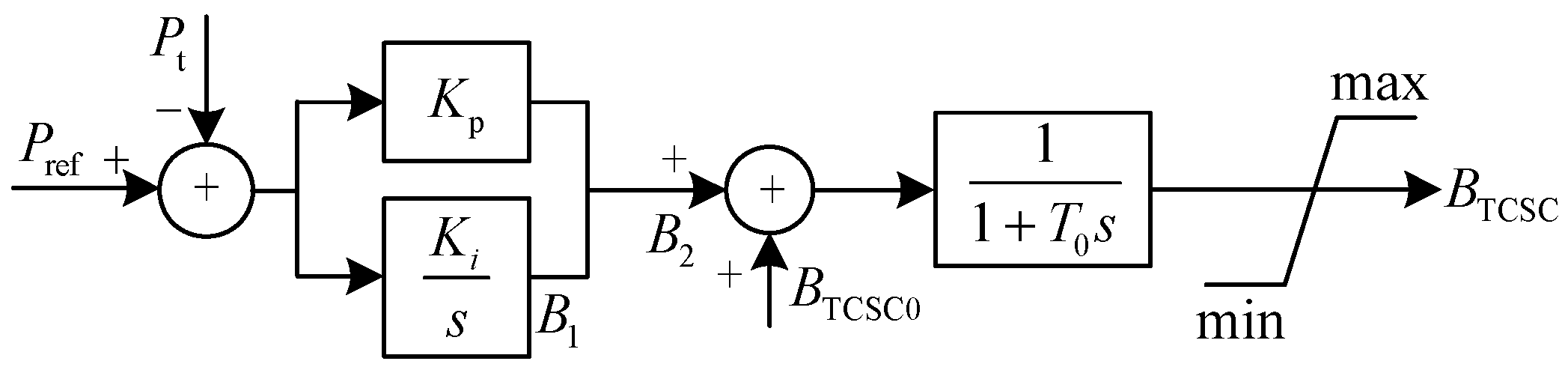
2.2. TCSC Model
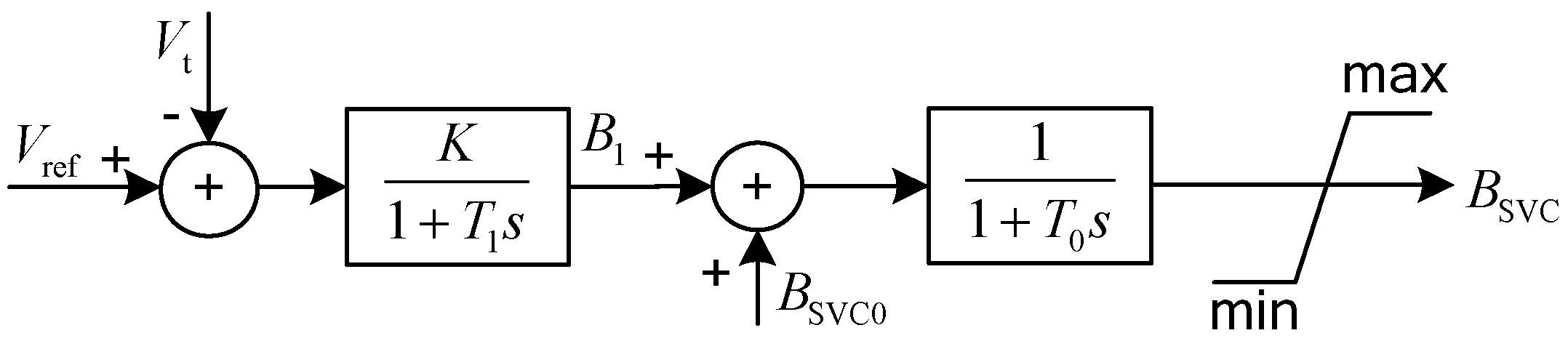
2.3. SVC Model
3. Main Results
3.1. Robust MFCC Design
3.2 Time-Delay MFCC Design
4. Numerical Simulations
5. Conclusions
Acknowledgments
Author Contributions
Conflicts of Interest
References
- Klein, M.; Rogers, G.; Kundur, P. A fundamental study of inter-area oscillations in power systems. IEEE Trans. Power Syst. 1991, 6, 914–921. [Google Scholar] [CrossRef]
- Kamwa, I.; Grondin, G.; Hebert, Y. Wide-area measurement based stabilizing control of large power systems—A decentralized/hierarchical approach. IEEE Trans. Power Syst. 2001, 16, 136–153. [Google Scholar] [CrossRef]
- Paserba, J. Analysis and Control of Power System Oscillations; CIGRE Special Publication 38.01.07, Technical Brochure III; International Council on Large Electric Systems (CIGRE): Paris, France, 1996. [Google Scholar]
- Tedesco, F.; Casavola, A. Fault-tolerant distributed load/frequency supervisory strategies for networked multi-area microgrids. Int. J. Robust Nonlinear Control 2014, 24, 1380–1402. [Google Scholar] [CrossRef]
- Magdy, E.; Sallam, A.; McCalley, J.; Fouad, A.A. Damping controller design for power system oscillation. IEEE Trans. Power Syst. 1996, 11, 767–773. [Google Scholar]
- De Oliveira, R.V.; Kuiava, R.; Ramos, R.A.; Bretas, N.G. Automatic tuning method for the design of supplementary damping controllers for flexible alternating current transmission system devices. IET Gener. Transm. Distrib. 2009, 3, 919–929. [Google Scholar] [CrossRef]
- Simfukwe, D.D.; Pal, B.C.; Jabr, R.A.; Martins, N. Robust and low-order design of flexible AC transmission systems and power system stabilisers for oscillation damping. IET Gener. Transm. Distrib. 2012, 6, 445–452. [Google Scholar] [CrossRef]
- Sanchez-Gasca, J.J. Coordinated control of two FACTS devices for damping interarea oscillations. IEEE Trans. Power Syst. 1998, 13, 428–434. [Google Scholar] [CrossRef]
- Noroozian, L.; Angquist, L.; Ghandhari, M.; Andersson, G. Improving power system dynamics by series-connected FACTS devices. IEEE Trans. Power Deliv. 1997, 12, 1635–1641. [Google Scholar] [CrossRef]
- Phadke, A.G. Synchronized phasor measurements in power system. IEEE Comput. Appl. Power 1993, 6, 10–15. [Google Scholar] [CrossRef]
- Deng, J.; Li, C.; Zhang, X.-P. Coordinated Design of Multiple Robust FACTS Damping Controllers: A BMI-Based Sequential Approach with Multi-Model Systems. IEEE Trans. Power Syst. 2015, 30, 3150–3159. [Google Scholar] [CrossRef]
- Leon, A.E.; Solsona, J.A. Power Oscillation Damping Improvement by Adding Multiple Wind Farms to Wide-Area Coordinating Controls. IEEE Trans. Power Syst. 2014, 29, 1356–1364. [Google Scholar] [CrossRef]
- Jiang, L.; Yao, W.; Wu, Q.H.; Wen, J.Y.; Cheng, S.J. Delay-dependent stability for load frequency control with constant and time-varying delays. IEEE Trans. Power Syst. 2012, 27, 932–941. [Google Scholar] [CrossRef]
- Wei, Y.; Jiang, L.; Wen, J.; Wu, Q.H.; Cheng, S. Wide-area damping controller of FACTS devices for inter-area oscillations considering communication time delays. IEEE Trans. Power Syst. 2014, 29, 318–329. [Google Scholar]
- Boyd, S.; El Ghaoui, L.; Feron, E.; Balakrishnan, V. Linear Matrix Inequalities in System and Control Theory; Society for Industrial and Applied Mathematics (SIAM): Philadelphia, PA, USA, 1994. [Google Scholar]
- Gahinet, P.; Nemirovski, A. LMI Control Toolbox for Use with MATLAB; Mathworks Inc.: Natick, MD, USA, 1995. [Google Scholar]
- Wu, M.; He, Y. Robust Control of Time-Delay System; Science Press: Beijing, China, 2007. [Google Scholar]
- Anderson, P.M.; Fouad, A.A. Power System Control and Stability; IEEE Press: Piscataway, NJ, USA, 1994. [Google Scholar]
- Hingorani, N.G.; Gyugyi, L. Understanding FACTS: Concepts and Technology of Flexible AC Transmission Systems; IEEE Press: New York, NY, USA, 2000. [Google Scholar]
- Del Rosso, D.; Canizares, C.A.; Dona, V.M. A study of TCSC controller design for power system stability improvement. IEEE Trans. Power Syst. 2003, 18, 1487–1496. [Google Scholar] [CrossRef]
- Zhou, K.; Doyle, J.C.; Golver, K. Robust and Optimal Control; Prentice Hall: Upper Saddle River, NJ, USA, 1995. [Google Scholar]
- Pal, B.C.; Coonick, A.H.; Jaimoukha, I.M.; El-Zobaidi, H. A linear matrix inequality approach to robust damping control design in power systems with superconducting magnetic energy storage device. IEEE Trans. Power Syst. 2000, 15, 356–362. [Google Scholar] [CrossRef] [Green Version]
- Kung, S.; Lin, D.W. Optimal Hankel-norm model reductions: Multivariable systems. IEEE Trans. Autom. Control 1981, 26, 832–852. [Google Scholar] [CrossRef]
- Chiali, M.; Bretas, P.G. H∞ design with pole placement constraints: An LMI approach. IEEE Trans. Autom. Control 1996, 41, 358–367. [Google Scholar] [CrossRef]
- Xu, S.Y.; Sun, H.D.; Li, B.Q.; Bu, G.Q. Wide-Area Robust Decentralized Coordinated Control of HVDC Power System Based on Polytopic System Theory. Math. Probl. Eng. 2015, 2015, 510216. [Google Scholar] [CrossRef]
- Oliveira, M.C.; Geromel, J.C.; Bernussou, J. Design of dynamic output feedback decentralized controllers via a separation procedure. Int. J. Control 2000, 73, 371–381. [Google Scholar] [CrossRef]
- Wu, M.; He, Y.; She, J.H.; Liu, G.P. Delay-dependent criteria for robust stability of time-varying delay systems. Automatica 2004, 40, 1435–1439. [Google Scholar] [CrossRef]
- Han, K.; Kim, H. Quantum-inspired evolutionary algorithm for a class of combinatorial optimization. IEEE Trans. Evol. Comput. 2002, 6, 580–593. [Google Scholar] [CrossRef]
- Bellen, A.; Maset, S. Numerical solution of constant coefficient linear delay differential equations as abstract Cauchy problems. Numer. Math. 2000, 84, 351–374. [Google Scholar] [CrossRef]
- Astrom, K.J.; Wittenmark, B. Computer-Controlled Systems-Theory and Design, 3rd ed.; Tsinghua University Press: Beijing, China, 2002; pp. 100–110. [Google Scholar]


| Modes | −0.018 ± j3.528 | −0.728 ± j6.324 | −0.789 ± j6.356 |
| Frequency/Hz | 0.562 | 1.006 | 1.012 |
| Damping Ratio | 0.524% | 11.443% | 12.319% |
| Description | Modes | Frequency/Hz | Damping Ratio | |
|---|---|---|---|---|
| Case 1 | Base Case | −0.018 ± j3.528 | 0.562 | 0.524% |
| −0.728 ± j6.324 | 1.006 | 11.443% | ||
| −0.789 ± j6.356 | 1.012 | 12.319% | ||
| Case 2 | Load 1: −100 MW Load 2: +100 MW | −0.008 ± j3.362 | 0.535 | 0.231% |
| −0.728 ± j6.291 | 1.002 | 11.495% | ||
| −0.779 ± j6.340 | 1.009 | 12.194% | ||
| Case 3 | Load 1: +100 MW Load 2: −100 MW | −0.028 ± j3.628 | 0.578 | 0.7614% |
| −0.725 ± j6.350 | 1.011 | 11.339% | ||
| −0.795 ± j6.364 | 1.012 | 12.402% |
| Description | Modes | Frequency/Hz | Damping Ratio | |
|---|---|---|---|---|
| Case 1 | Base Case | −0.675 ± j3.482 | 0.554 | 19.0319% |
| −0.715 ± j6.401 | 1.018 7 | 11.0982% | ||
| −0.816 ± j6.241 | 0.993 3 | 12.958% | ||
| Case 2 | Load 1: −100 MW Load 2: +100 MW | −0.699 ± j3.329 | 0.529 9 | 20.5334% |
| −0.711 ± j6.371 | 1.013 9 | 11.0872% | ||
| −0.809 ± j6.232 | 0.991 8 | 12.8706% | ||
| Case 3 | Load 1: +100 MW Load 2: −100 MW | −0.633 ± j3.552 | 0.565 3 | 17.5471% |
| −0.716 ± j6.420 | 1.021 8 | 11.0898% | ||
| −0.817 ± j6.247 | 0.994 2 | 12.9673% |
© 2017 by the authors. Licensee MDPI, Basel, Switzerland. This article is an open access article distributed under the terms and conditions of the Creative Commons Attribution (CC BY) license (http://creativecommons.org/licenses/by/4.0/).
Share and Cite
Xu, S.; Yang, Y.; Peng, K.; Li, L.; Hayat, T.; Alsaedi, A. Wide Area Coordinated Control of Multi-FACTS Devices to Damp Power System Oscillations. Energies 2017, 10, 2130. https://doi.org/10.3390/en10122130
Xu S, Yang Y, Peng K, Li L, Hayat T, Alsaedi A. Wide Area Coordinated Control of Multi-FACTS Devices to Damp Power System Oscillations. Energies. 2017; 10(12):2130. https://doi.org/10.3390/en10122130
Chicago/Turabian StyleXu, Shiyun, Ying Yang, Kaixiang Peng, Linlin Li, Tasawar Hayat, and Ahmed Alsaedi. 2017. "Wide Area Coordinated Control of Multi-FACTS Devices to Damp Power System Oscillations" Energies 10, no. 12: 2130. https://doi.org/10.3390/en10122130
APA StyleXu, S., Yang, Y., Peng, K., Li, L., Hayat, T., & Alsaedi, A. (2017). Wide Area Coordinated Control of Multi-FACTS Devices to Damp Power System Oscillations. Energies, 10(12), 2130. https://doi.org/10.3390/en10122130