Comparative Performance Analysis of Optimal PID Parameters Tuning Based on the Optics Inspired Optimization Methods for Automatic Generation Control


Abstract
:1. Introduction
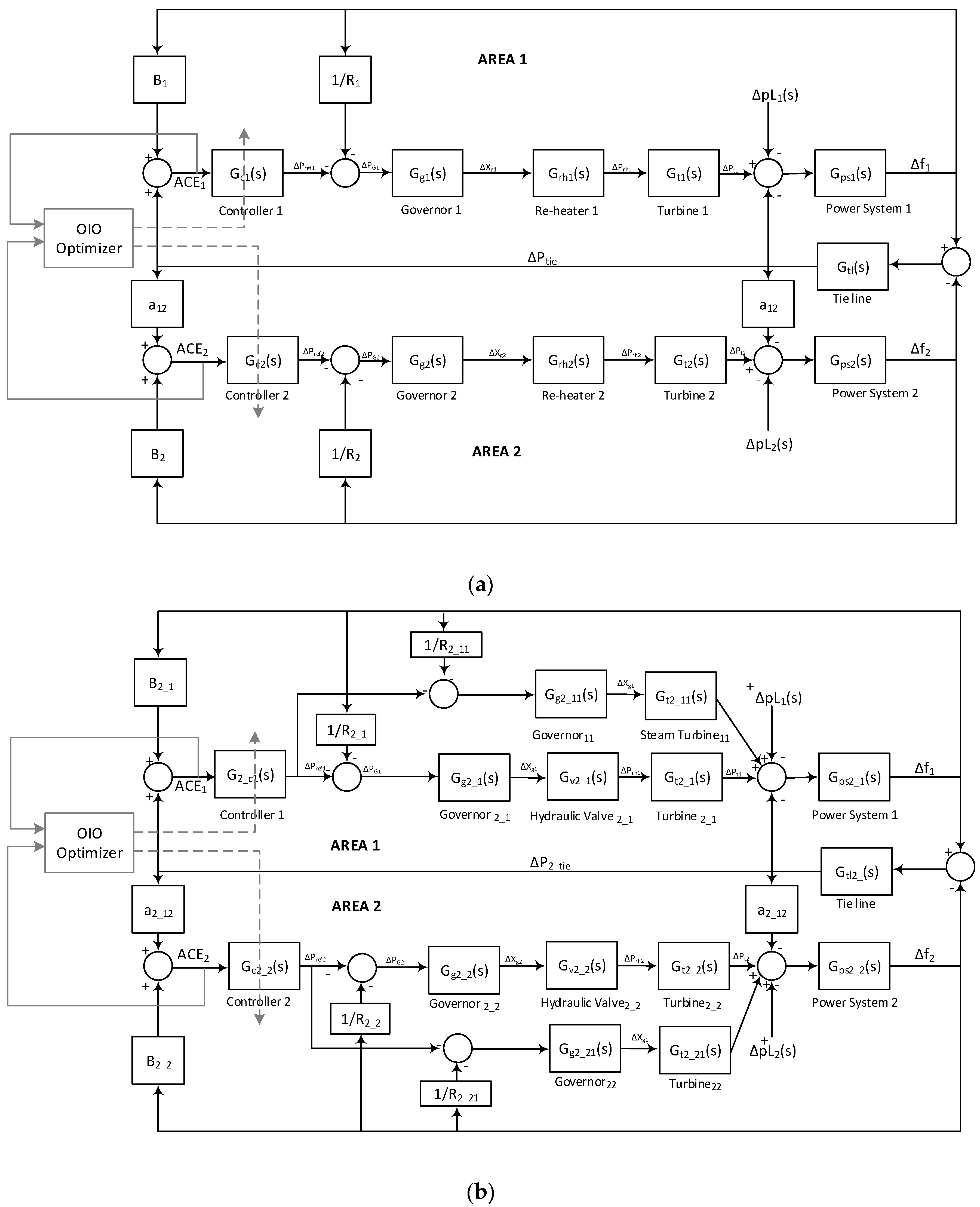
2. Power System Model
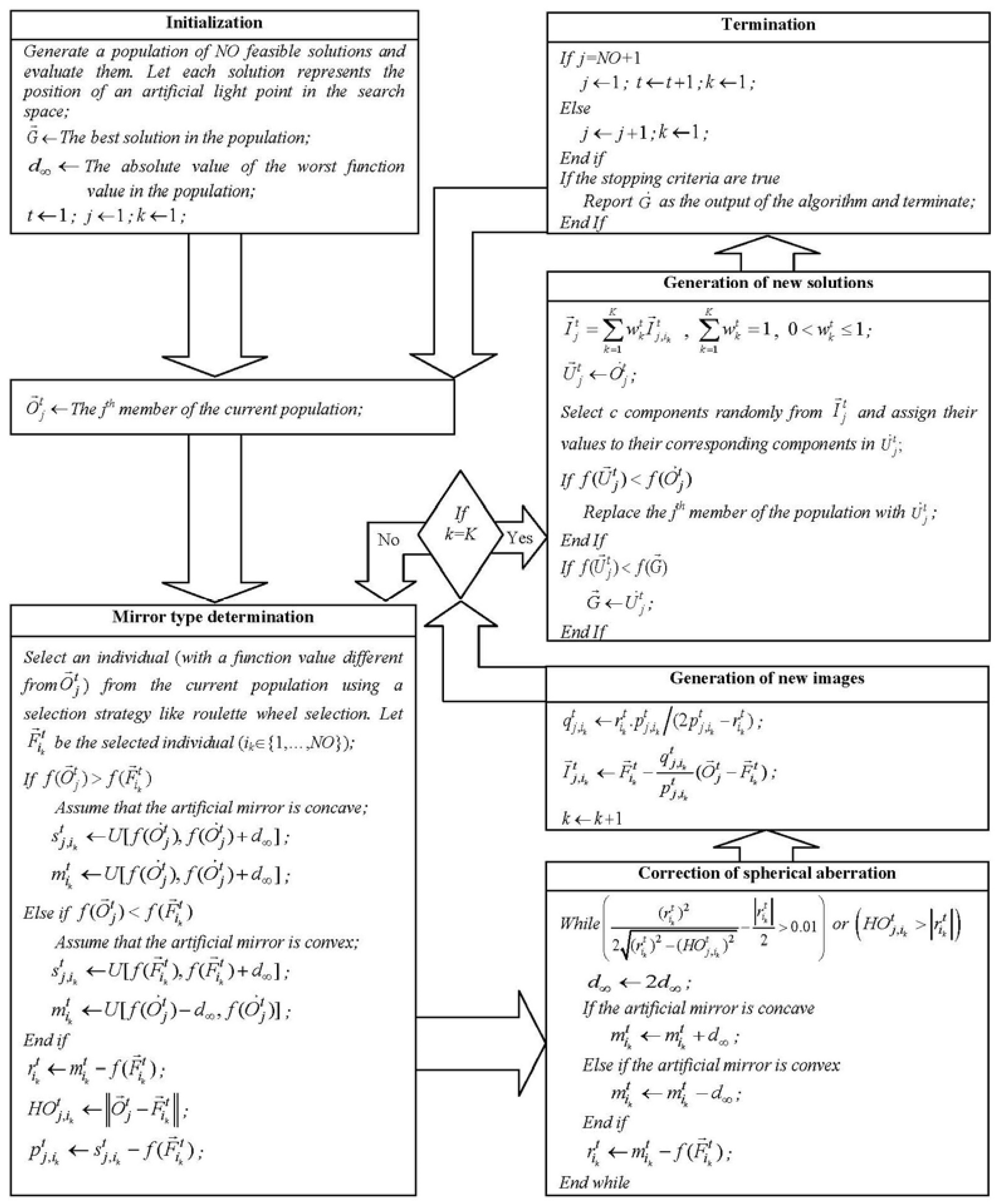
3. Optics Inspired Optimization
- -
- indicates the position of j artificial point of light in the t iteration and n-dimensional space (i.e., j th solution in the population).
- -
- specifies a different point in the search space passing through its own artificial axis (an individual in position). Artificial mirror peak position is determined by vector. index is randomly selected from NO is the number of artificial light points.
- -
- specifies location of an image of j artificial point of light in the t iteration in the search space. The artificial image is created through by an artificial mirror passing through the main axis.
- -
- specifies the position of j artificial light point on function/objective axis (objective space) in t iteration. The position of j artificial light point in common search and objective space is given by vector.
- -
- is the distance between j artificial light point on function/objective axis (objective space) and vertex of the artificial mirror in t iteration.
- -
- is the distance between j artificial light point on function/objective axis and position of vertex of the artificial mirror on function/objective axis .
- -
- is the radius of curvature of an artificial mirror that can pass through the center of curvature of an artificial mirror on the main axis through .
- -
- is the position of the center of curvature on function/objective axis (in the objective space).
- -
- is the height of j artificial light point from the artificial main axis in t iteration.
- -
- is the height of image of j artificial light point from the artificial main axis in t iteration.
- -
- is the value of lateral deviation on artificial mirror reflecting the image of j artificial light point in t iteration.
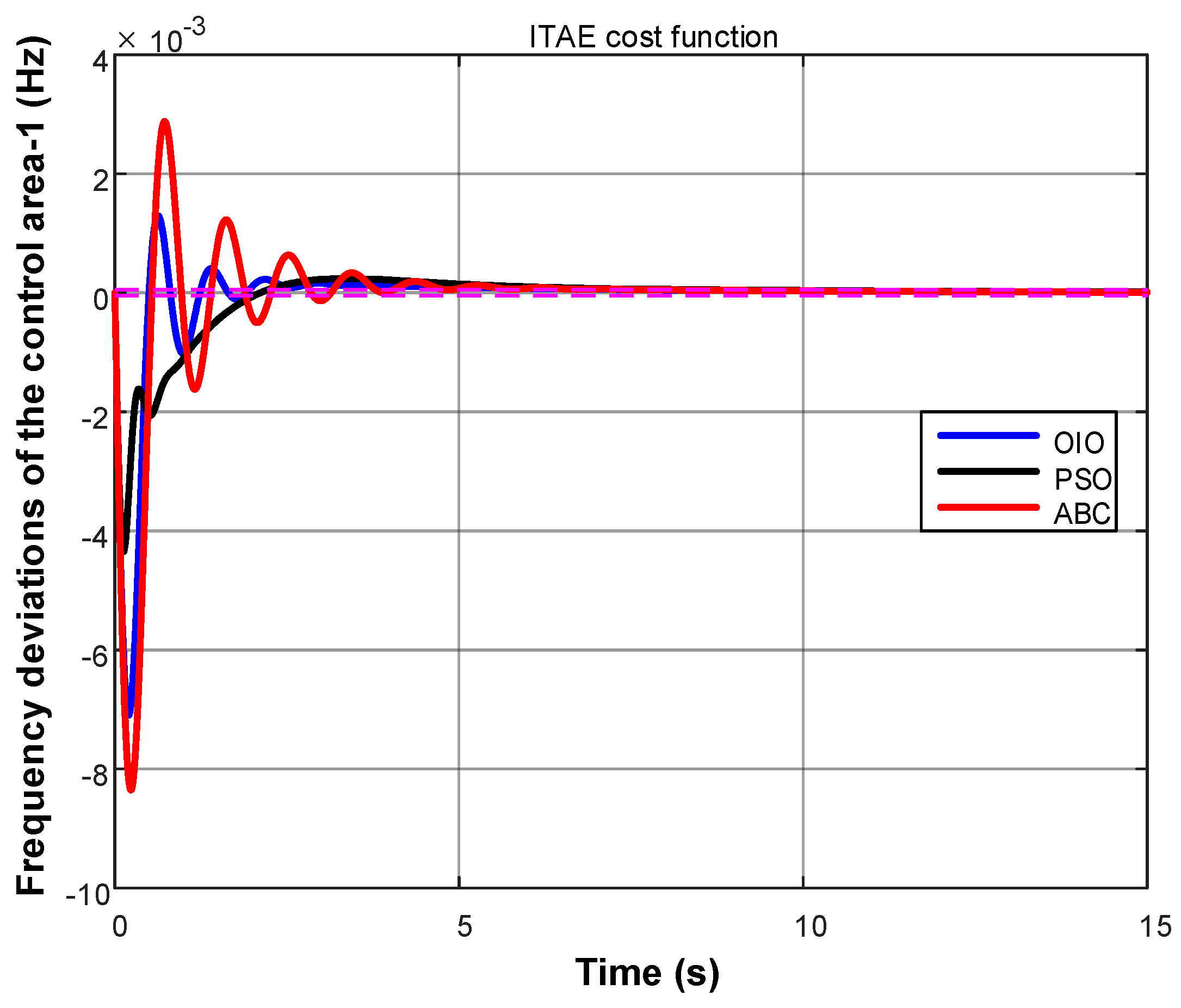
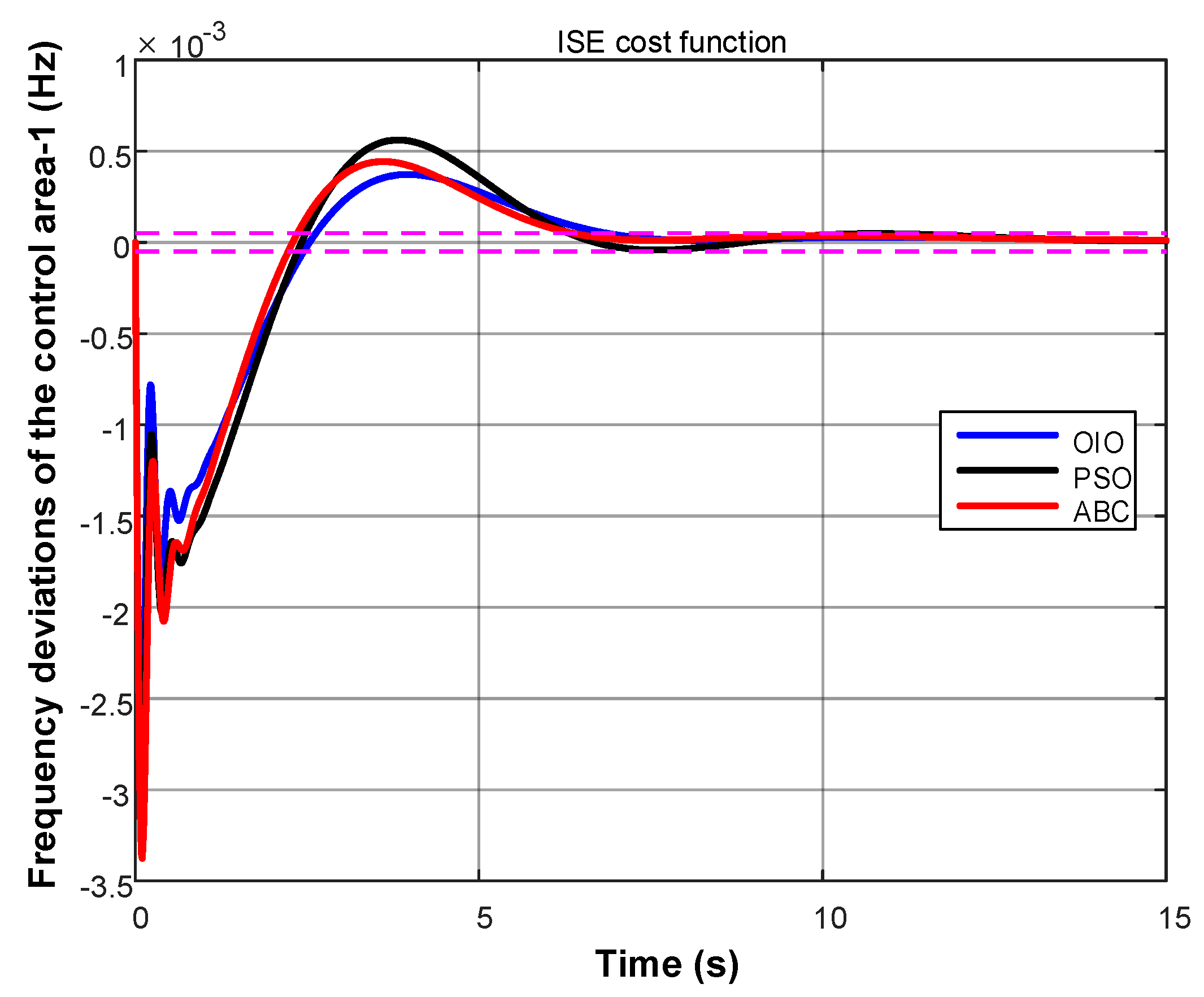
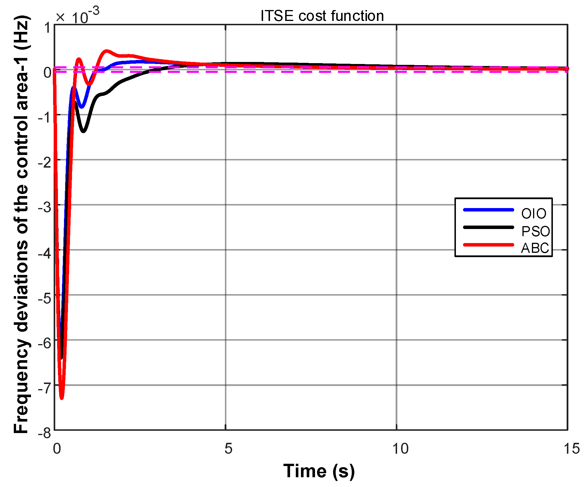
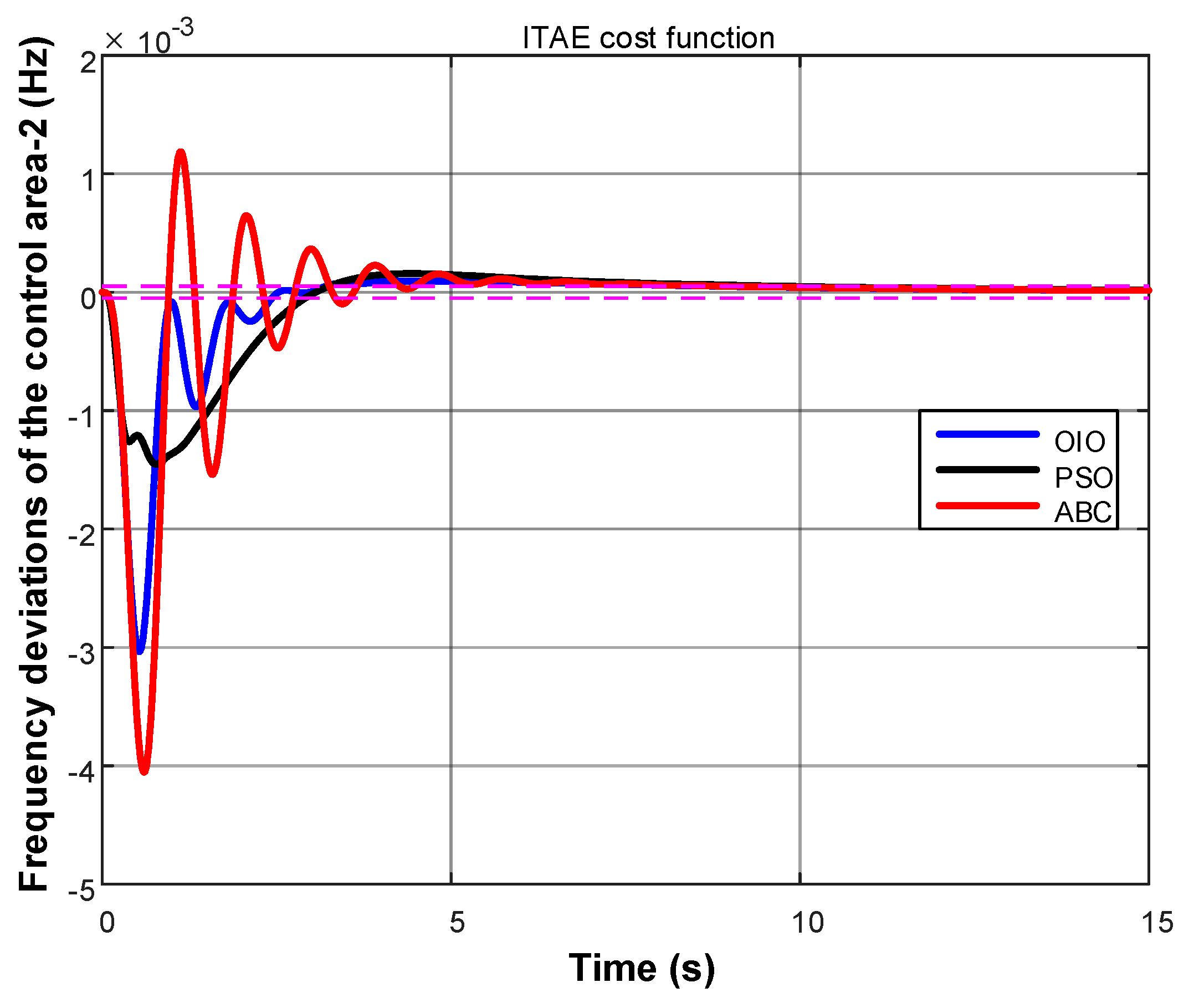
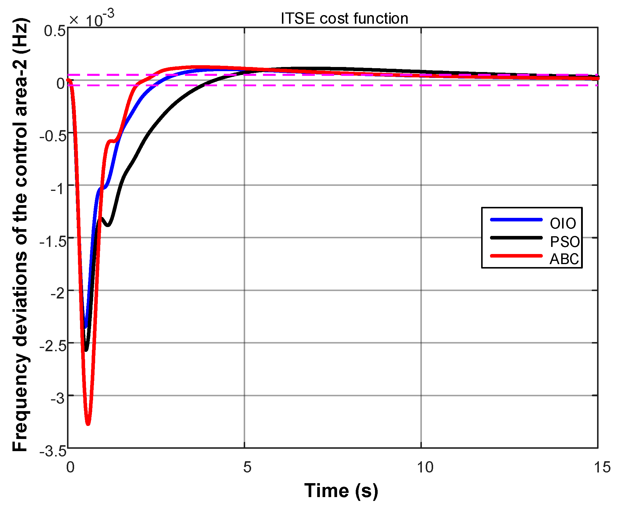
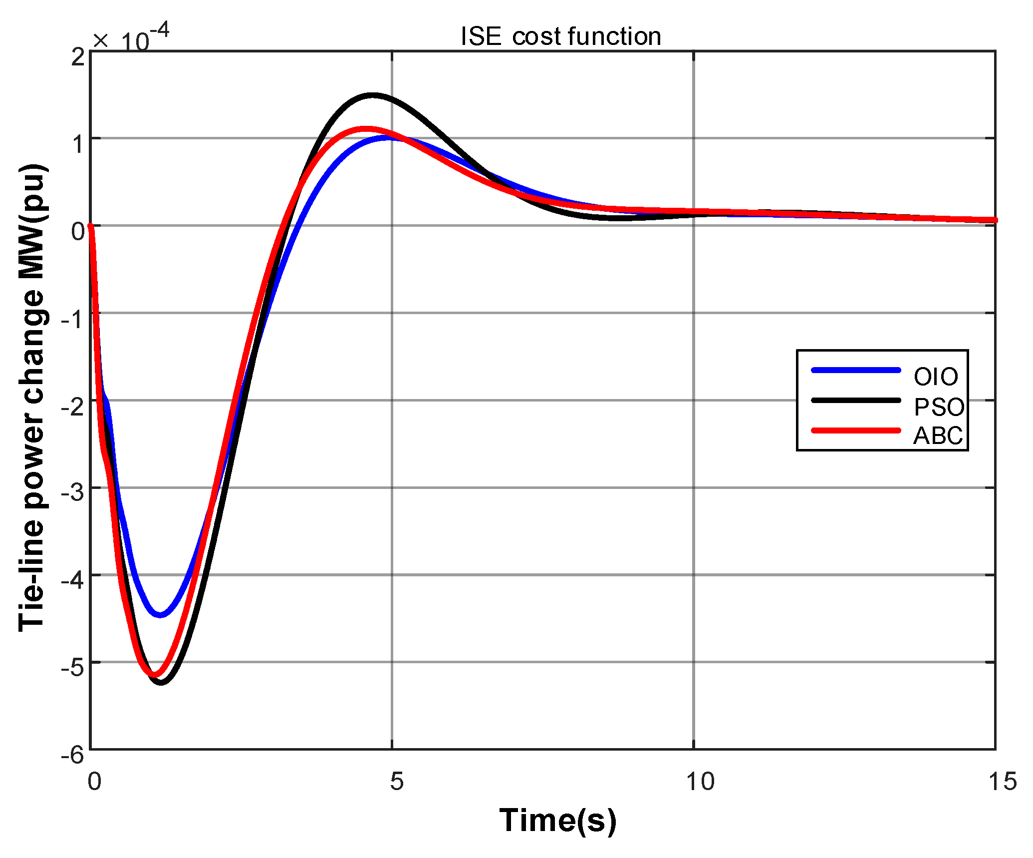
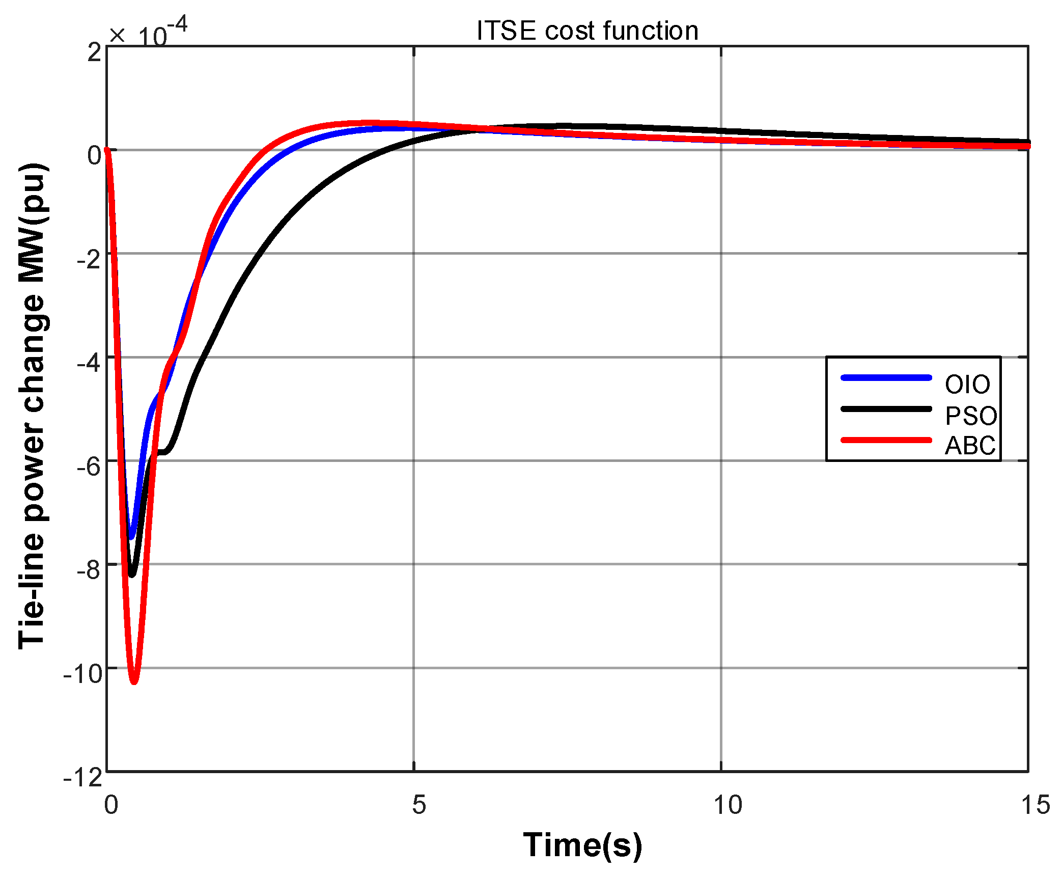
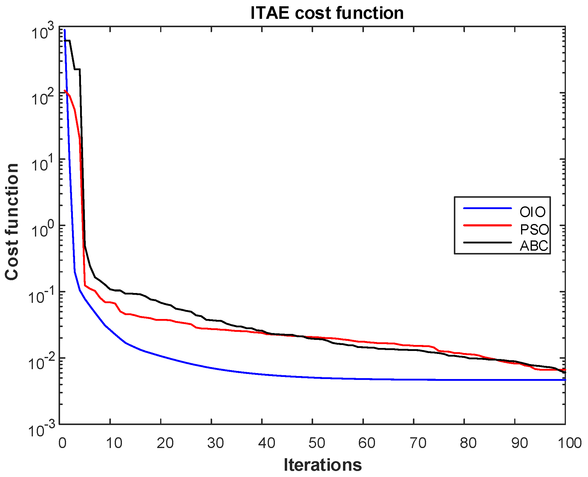
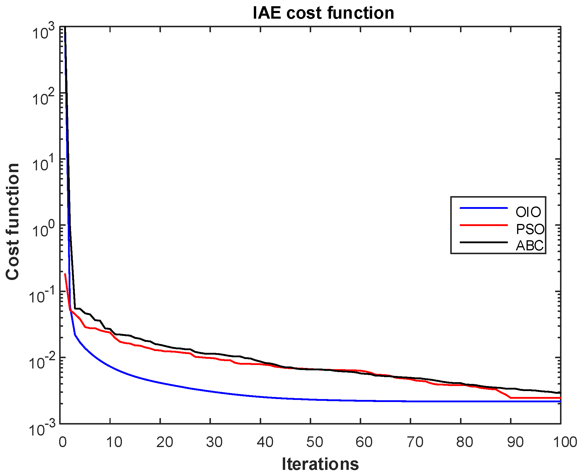
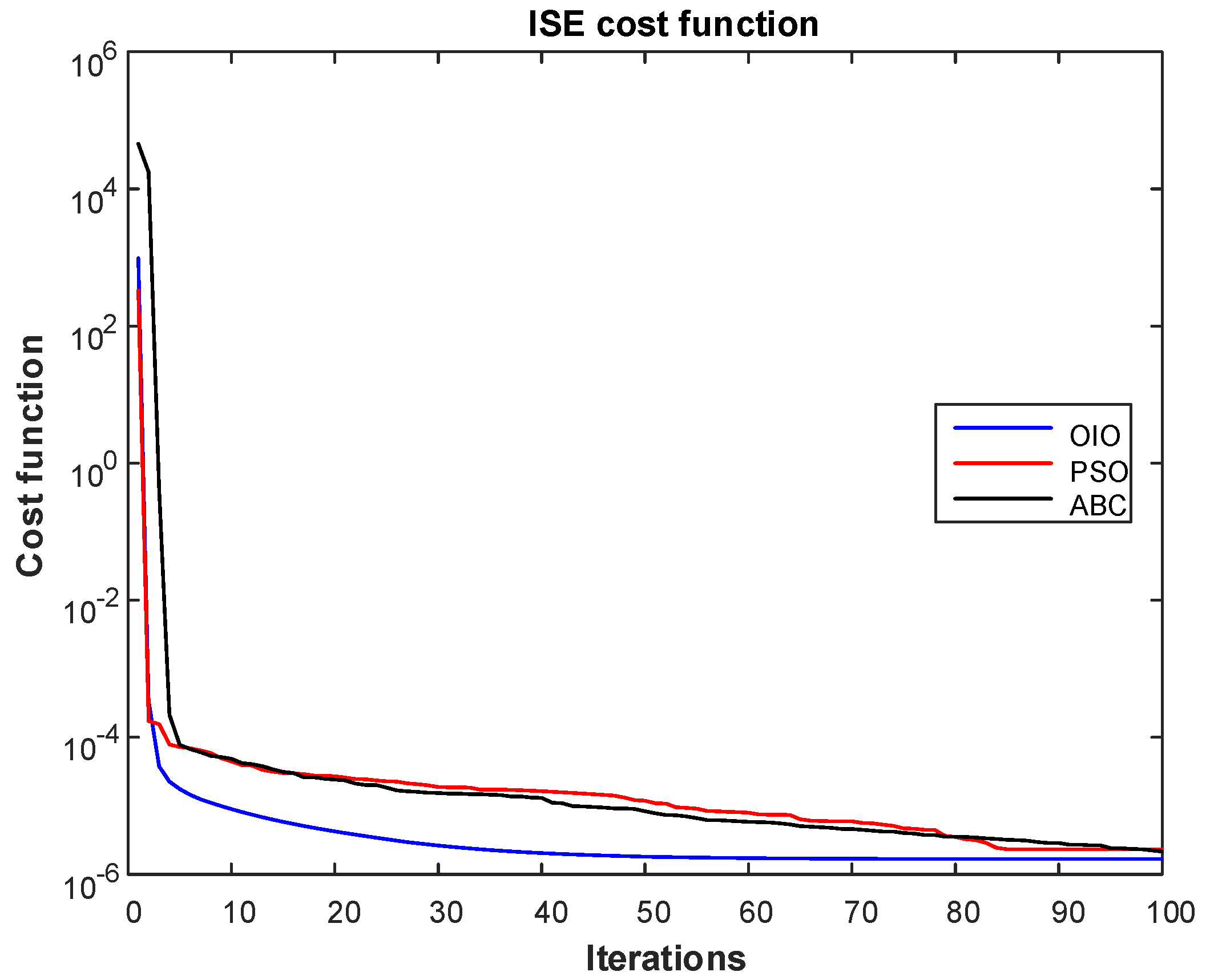
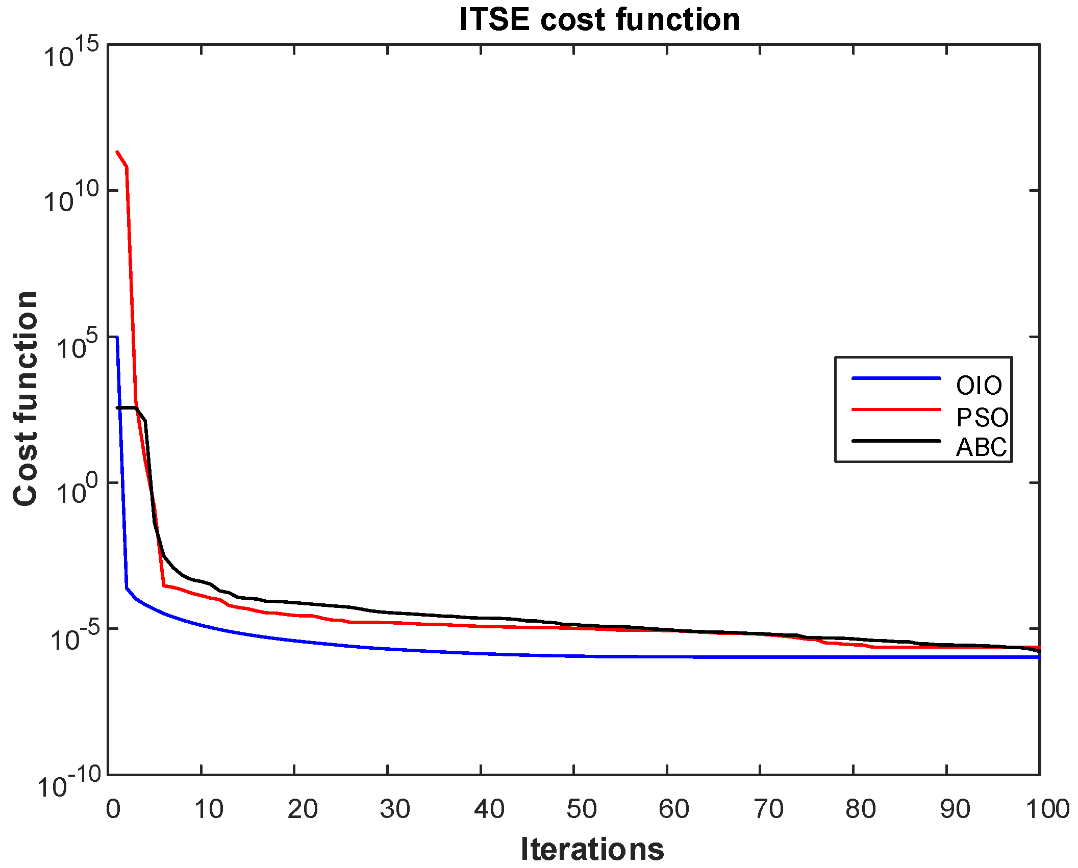
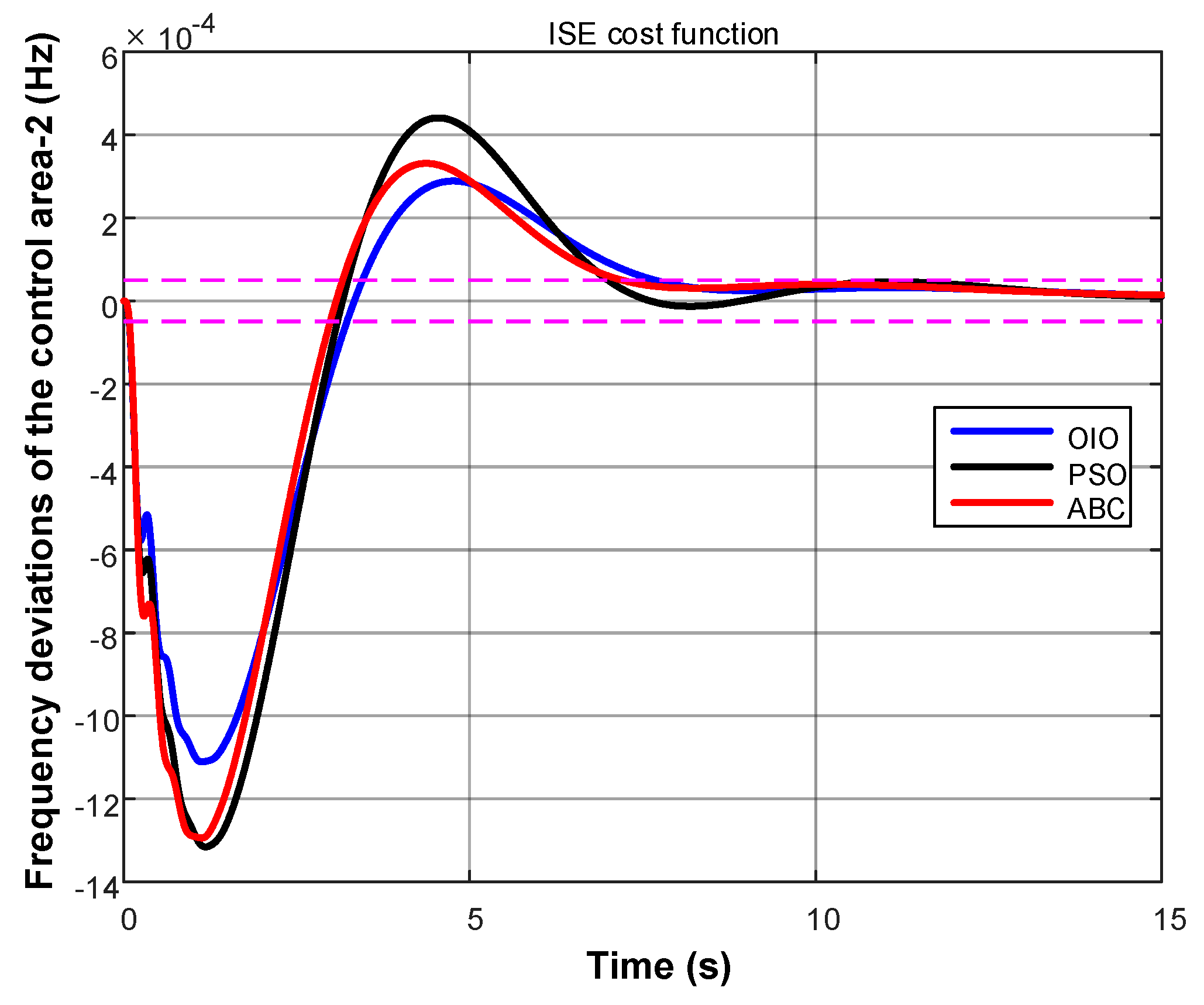
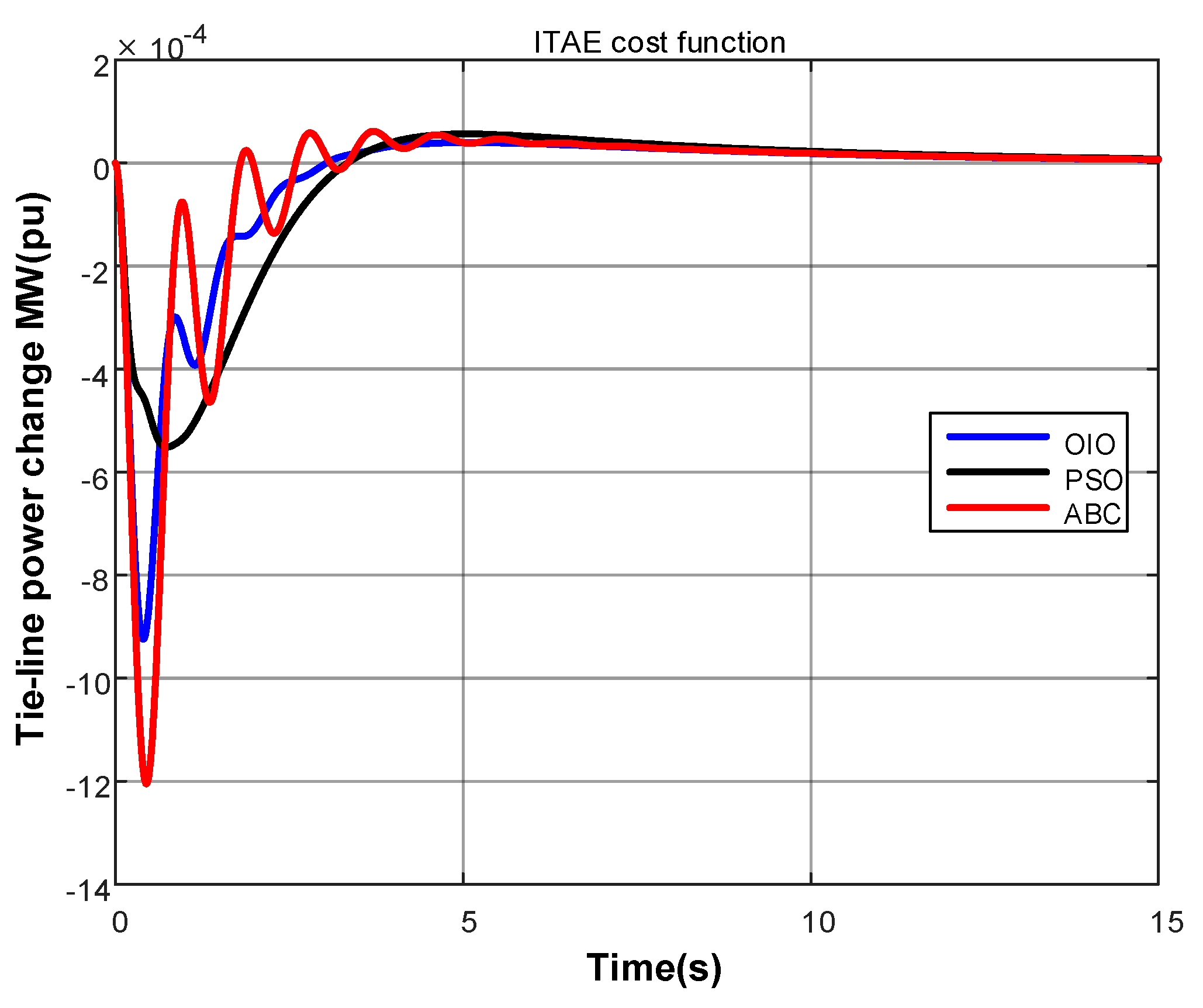
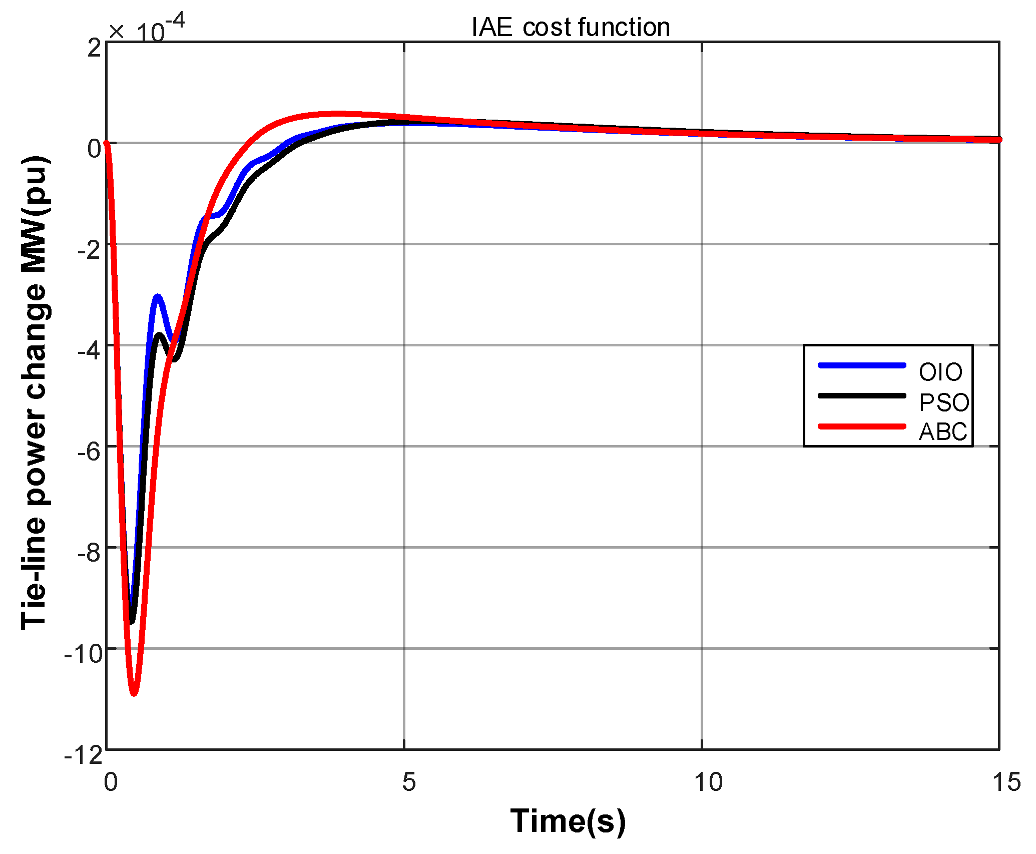
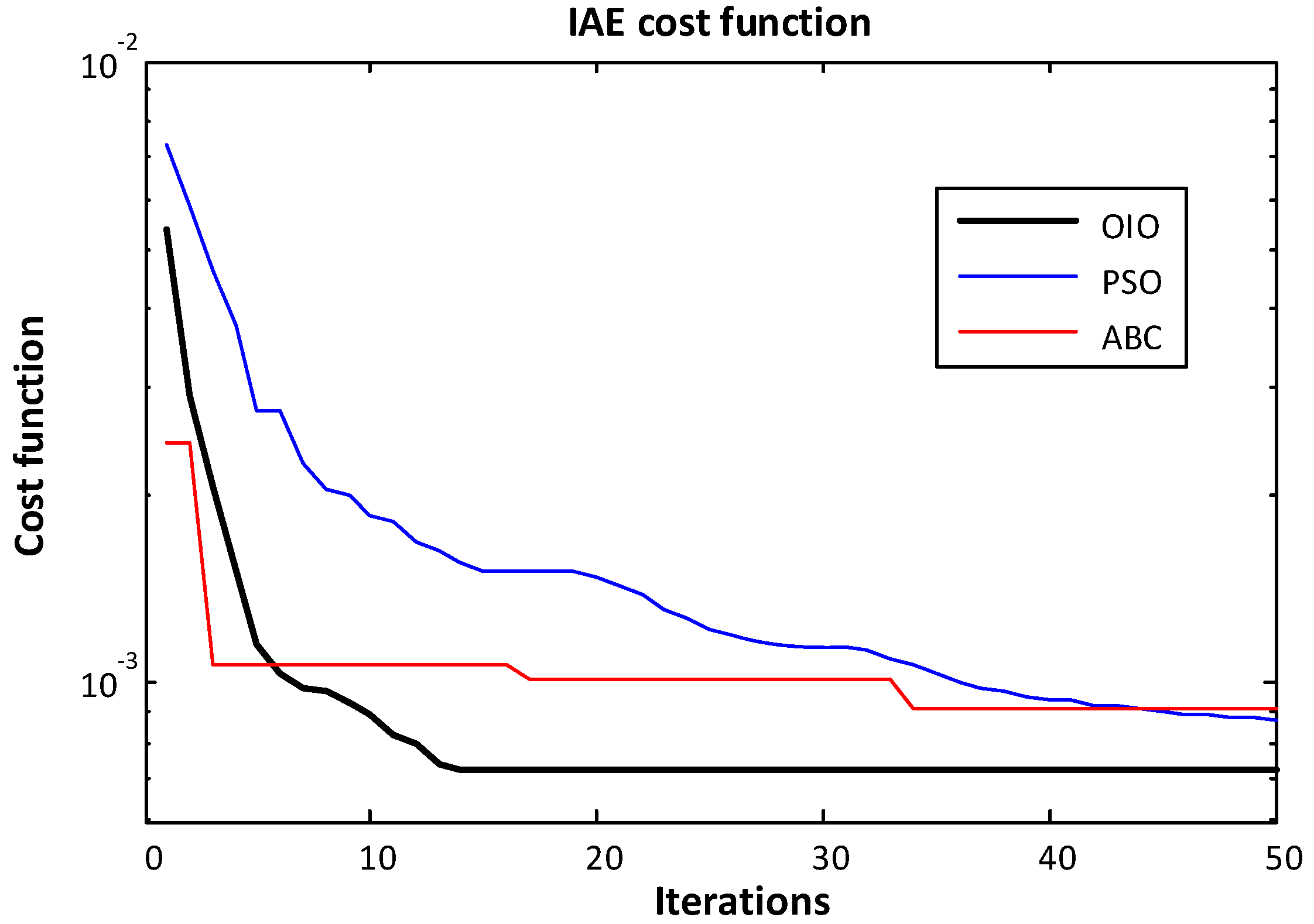
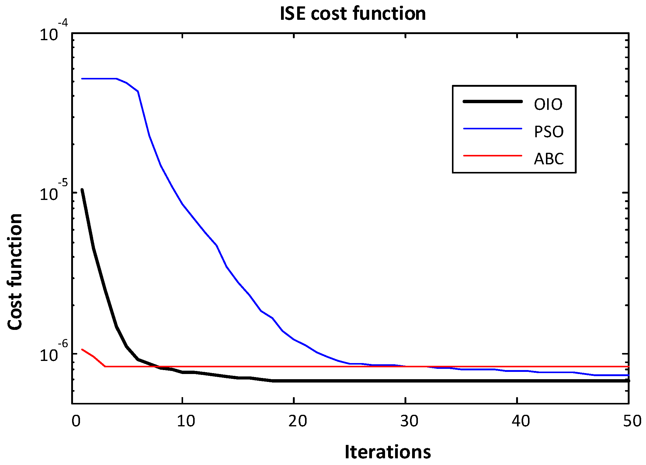
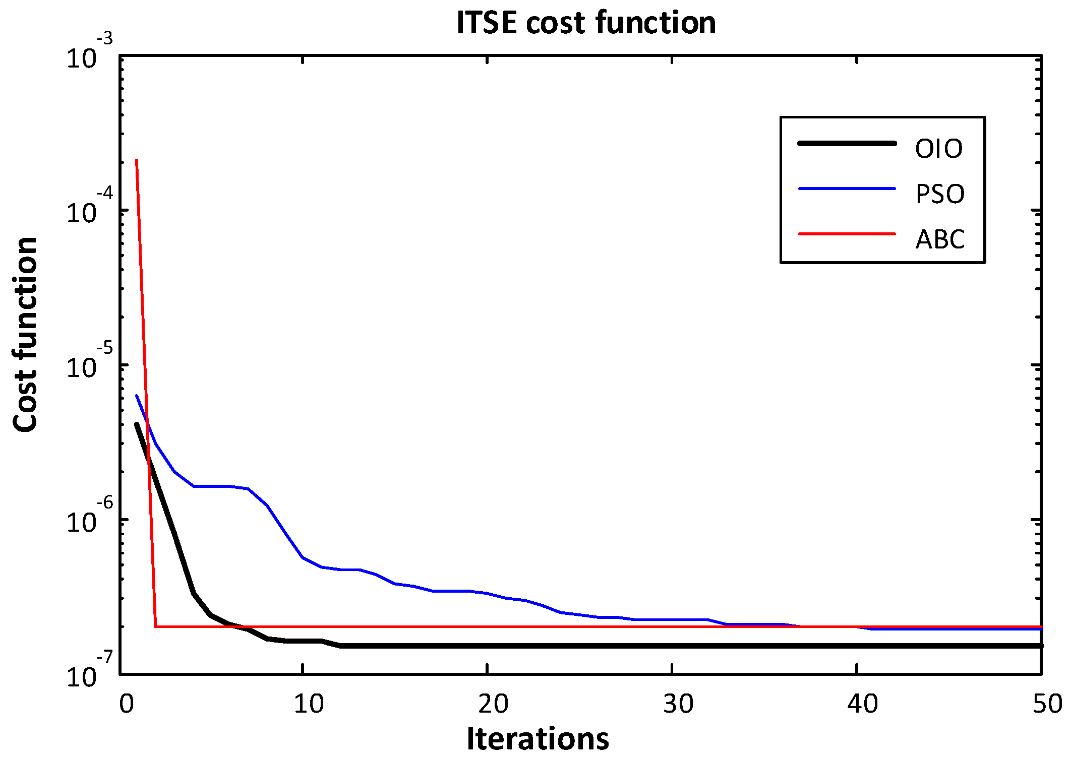
4. Results
- Integral of square error (ISE)
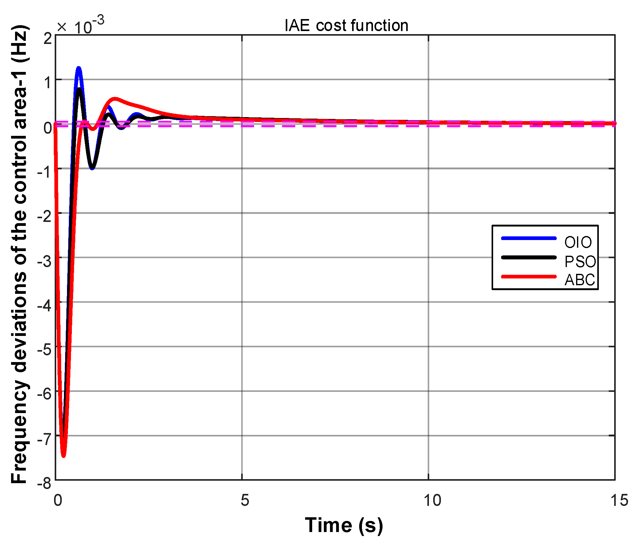
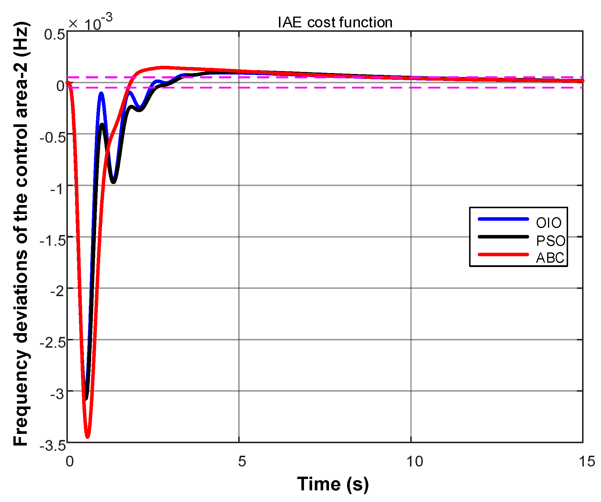
- Integral of absolute value of error (IAE)
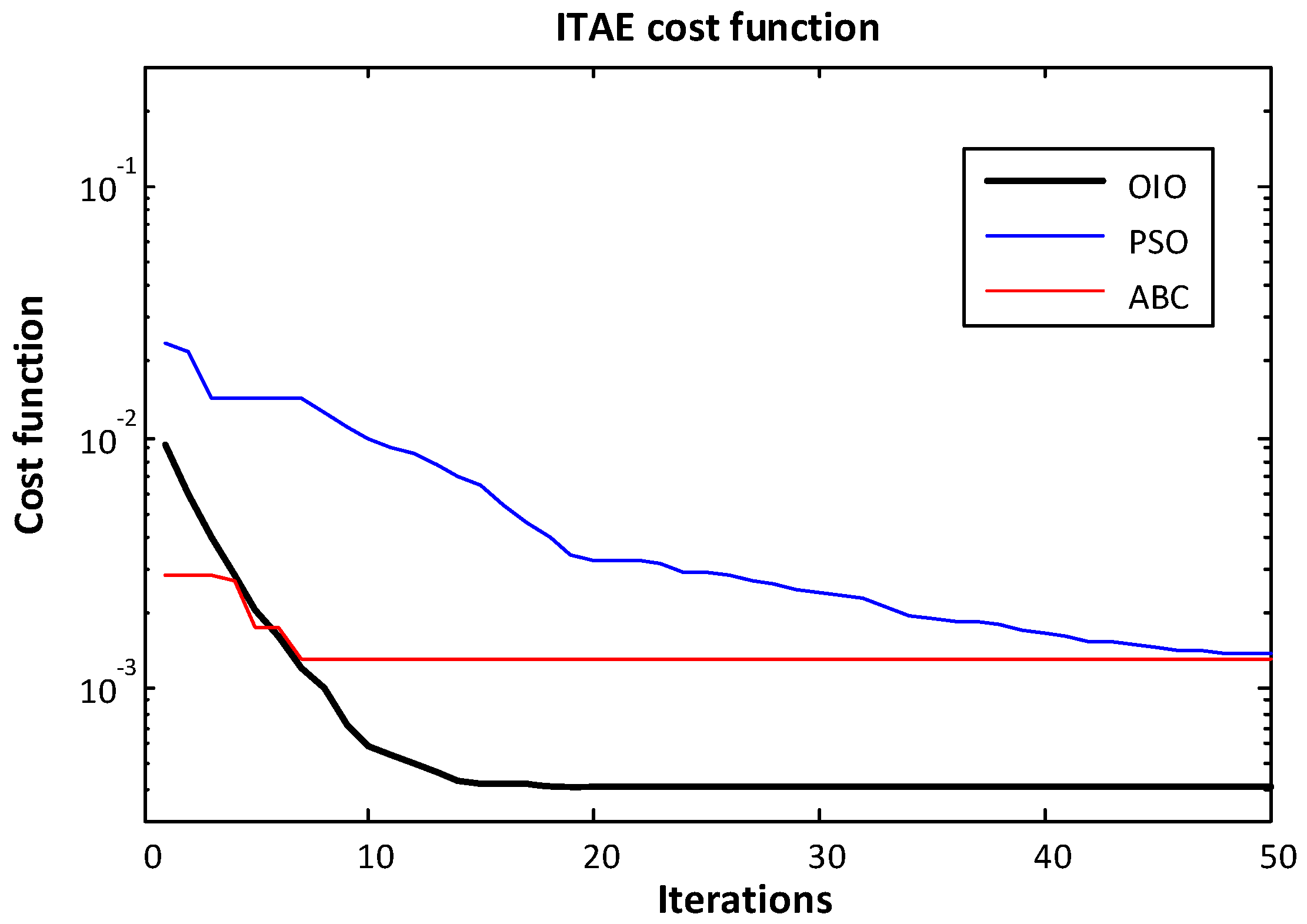
- Time-weighted ITAE
- Time-weighted ITSE
5. Conclusions
- OIO algorithm has found lowest cost value.
- OIO algorithm reaches to the global minimum value in short time.
- OIO can converge with less number of population.
- OIO algorithm has the total lowest optimization time.
Author Contributions
Conflicts of Interest
Appendix A
References
- Kundur, P. Power System Control and Stability; McGraw-Hill: New York, NY, USA, 1994. [Google Scholar]
- Özdemir, M.T.; Öztürk, D.; Eke, İ.; Çelik, V.; Lee, K. Tuning of Optimal Classical and Fractional Order PID Parameters for Automatic Generation Control Based on the Bacterial Swarm Optimization. IFAC-PapersOnLine 2015, 48, 501–506. [Google Scholar] [CrossRef]
- Eberhart, R.; Kennedy, J. A new optimizer using particle swarm theory. In Proceedings of the Sixth International Symposium on Micro Machine and Human Science (MHS ’95), Nagoya, Japan, 4–6 October 1995; pp. 39–43. [Google Scholar]
- Geem, Z.; Kim, J.; Loganathan, G.V. A New Heuristic Optimization Algorithm: Harmony Search. Simulation 2001, 76, 60–68. [Google Scholar] [CrossRef]
- Passino, K.M. Biomimicry of bacterial foraging for distributed optimization and control. IEEE Control Syst. Mag. 2002, 22, 52–67. [Google Scholar] [CrossRef]
- Muller, S.D.; Marchetto, J.; Airaghi, S.; Kournoutsakos, P. Optimization based on bacterial chemotaxis. IEEE Trans. Evol. Comput. 2002, 6, 16–29. [Google Scholar] [CrossRef]
- Karaboga, D. An Idea Based on Honey Bee Swarm for Numerical Optimization; Technical Report TR06; Erciyes University: Kayseri, Turkey, 2005. [Google Scholar]
- Formato, R.A. Central Force Optimization: A New Metaheuristic with Applications in Applied Electromagnetics. Prog. Electromagn. Res. 2007, 77, 425–491. [Google Scholar] [CrossRef]
- Yang, X.S. Firefly algorithm, stochastic test functions and design optimization. Int. J. Bio-Inspir. Comput. 2010, 2, 78–84. [Google Scholar] [CrossRef]
- Kashan, A.H. League Championship Algorithm: A new algorithm for numerical function optimization. In Proceedings of the International Conference of Soft Computing and Pattern Recognition (SoCPaR 2009), Malacca, Malaysia, 4–7 December 2009; pp. 43–48. [Google Scholar]
- He, S.; Wu, Q.H.; Saunders, J.R. Group search optimizer: An optimization algorithm inspired by animal searching behavior. IEEE Trans. Evol. Comput. 2009, 13, 973–990. [Google Scholar] [CrossRef]
- Rashedi, E.; Nezamabadi-Pour, H.; Saryazdi, S. GSA: A Gravitational Search Algorithm. Inf. Sci. 2009, 179, 2232–2248. [Google Scholar] [CrossRef]
- Rao, R.V.; Savsani, V.J.; Vakharia, D.P. Teaching–learning-based optimization: A novel method for constrained mechanical design optimization problems. Comput.-Aided Des. 2011, 43, 303–315. [Google Scholar] [CrossRef]
- Gandomi, A.H.; Alavi, A.H. Krill herd: A new bio-inspired optimization algorithm. Commun. Nonlinear Sci. Numer. Simul. 2012, 17, 4831–4845. [Google Scholar] [CrossRef]
- Lu, Q.-Y.; Hu, W.; Zheng, L.; Min, Y.; Li, M.; Li, X.; Ge, W.; Wang, Z. Integrated Coordinated Optimization Control of Automatic Generation Control and Automatic Voltage Control in Regional Power Grids. Energies 2012, 5, 3817–3834. [Google Scholar] [CrossRef]
- Muñoz-Benavente, I.; Gómez-Lázaro, E.; García-Sánchez, T.; Vigueras-Rodríguez, A.; Molina-García, A. Implementation and Assessment of a Decentralized Load Frequency Control: Application to Power Systems with High Wind Energy Penetration. Energies 2017, 10, 151. [Google Scholar] [CrossRef]
- Song, J.; Pan, X.; Lu, C.; Xu, H. A Simulation-Based Optimization Method for Hybrid Frequency Regulation System Configuration. Energies 2017, 10, 1302. [Google Scholar] [CrossRef]
- Huang, C.; Yue, D.; Xie, X.; Xie, J. Anti-Windup Load Frequency Controller Design for Multi-Area Power System with Generation Rate Constraint. Energies 2016, 9, 330. [Google Scholar] [CrossRef]
- Mohanty, B. TLBO optimized sliding mode controller for multi-area multi-source nonlinear interconnected AGC system. Int. J. Electr. Power Energy Syst. 2015, 73, 872–881. [Google Scholar] [CrossRef]
- Zeng, G.-Q.; Xie, X.-Q.; Chen, M.-R. An Adaptive Model Predictive Load Frequency Control Method for Multi-Area Interconnected Power Systems with Photovoltaic Generations. Energies 2017, 10, 1840. [Google Scholar] [CrossRef]
- Surender, R.S.; Srinivasa Rathnam, C. Optimal Power Flow using Glowworm Swarm Optimization. Int. J. Electr. Power Energy Syst. 2016, 80, 128–139. [Google Scholar] [CrossRef]
- Reddy, S.S. Solution of multi-objective optimal power flow using efficient meta-heuristic algorithm. Electr. Eng. 2017. [Google Scholar] [CrossRef]
- Surenderr, R.S.; Bijwe, P.R.; Abhyankar, A.R. Faster evolutionary algorithm based optimal power flow using incremental variables. Int. J. Electr. Power Energy Syst. 2014, 54, 198–210. [Google Scholar] [CrossRef]
- Ali, E.S.; Abd-Elazim, S.M. Bacteria foraging optimization algorithm based load frequency controller for interconnected power system. Int. J. Electr. Power Energy Syst. 2011, 33, 633–638. [Google Scholar] [CrossRef]
- Saikia, L.C.; Nanda, J.; Mishra, S. Performance comparison of several classical controllers in AGC for multi-area interconnected thermal system. Int. J. Electr. Power Energy Syst. 2011, 33, 394–401. [Google Scholar] [CrossRef]
- Özdemir, M.T.; Öztürk, D. Optimal Load frequency control in two area power systems with Optics Inspired Optimization. Firat Universitesi Muhendislik Bilimleri Dergisi 2016, 2, 57–66. [Google Scholar]
- Muñoz, M.A.; Halgamuge, S.K.; Alfonso, W.; Caicedo, E.F. Simplifying the bacteria foraging optimization algorithm. In Proceedings of the 2010 IEEE Congress on Evolutionary Computation (CEC), Barcelona, Spain, 18–23 July 2010. [Google Scholar]
- Yousuf, M.S.; Al-Duwaish, H.N.; Al-Hamouz, Z.M. PSO based single and two interconnected area predictive automatic generation control. WSEAS Trans. Syst. Control 2010, 5, 677–690. [Google Scholar]
- Gozde, H.; Taplamacioglu, M.C. Automatic generation control application with craziness based particle swarm optimization in a thermal power system. Int. J. Electr. Power Energy Syst. 2011, 33, 8–16. [Google Scholar] [CrossRef]
- Serbet, F.; Kaya, T.; Ozdemir, M.T. Design of digital IIR filter using Particle Swarm Optimization. In Proceedings of the 2017 40th International Convention on Information and Communication Technology, Electronics and Microelectronics, Opatija, Croatia, 22–26 May 2017. [Google Scholar]
- Panda, S.; Mohanty, B.; Hota, P.K. Hybrid BFOA–PSO algorithm for automatic generation control of linear and nonlinear interconnected power systems. Appl. Soft Comput. 2013, 13, 4718–4730. [Google Scholar] [CrossRef]
- Özdemir, M.T.; Yildirim, B.; Gülan, H.; Gençoğlu, M.T.; Cebeci, M. Automatic Generation Control in an AC Isolated Microgrid using the League Championship. Fırat Üniversitesi Mühendislik Bilimleri Dergisi 2017, 29, 109–120. [Google Scholar]
- Özdemir, M.T.; Yıldız, S. Effects of High Voltage Direct Current Transmission Lines on Load Frequency Control in a Multi Area Power System. In Proceedings of the Güç Sistemleri Konferansı, Istanbul, Turkey, 15–16 November 2016; pp. 1–5. [Google Scholar]
- Hsiao, Y.; Chuang, C.; Chien, C. Ant colony optimization for designing of PID controllers. In Proceedings of the 2004 IEEE International Conference on Robotics and Automation, New Orleans, LA, USA, 2–4 September 2004; IEEE Cat. No.04CH37508. pp. 321–326. [Google Scholar]
- Naidu, K.; Mokhlis, H.; Bakar, A.H.A. Multiobjective optimization using weighted sum Artificial Bee Colony algorithm for Load Frequency Control. Int. J. Electr. Power Energy Syst. 2014, 55, 657–667. [Google Scholar] [CrossRef]
- Eke, İ.; Taplamacıoğlu, M.C.; Lee, K.Y. Robust Tuning of Power System Stabilizer by Using Orthogonal Learning Artificial Bee Colony. IFAC-PapersOnLine 2015, 48, 149–154. [Google Scholar] [CrossRef]
- Kashan, A.H. An effective algorithm for constrained optimization based on optics inspired optimization (OIO). CAD Comput. Aided Des. 2015, 63, 52–71. [Google Scholar] [CrossRef]
- Husseinzadeh Kashan, A. A new metaheuristic for optimization: Optics inspired optimization (OIO). Comput. Oper. Res. 2014, 55, 99–125. [Google Scholar] [CrossRef]
- Çelik, V.; Özdemir, M.T.; Bayrak, G. The effects on stability region of the fractional-order PI controller for one-area time-delayed load-frequency control systems. Trans. Inst. Meas. Control 2016. [Google Scholar] [CrossRef]
- Çam, E. Application of fuzzy logic for load frequency control of hydroelectrical power plants. Energy Convers. Manag. 2007, 48, 1281–1288. [Google Scholar] [CrossRef]
- Guha, D.; Roy, P.K.; Banerjee, S. Load frequency control of interconnected power system using grey wolf optimization. Swarm Evol. Comput. 2016, 27, 97–115. [Google Scholar] [CrossRef]
- Vijaya Chandrakala, K.R.M.; Balamurugan, S.; Sankaranarayanan, K. Variable structure fuzzy gain scheduling based load frequency controller for multi source multi area hydro thermal system. Int. J. Electr. Power Energy Syst. 2013, 53, 375–381. [Google Scholar] [CrossRef]


| Controller Gain Limits | Kp | Ki | Kd |
|---|---|---|---|
| Upper Limits | 0 | 0 | 0 |
| Lower Limits | 10 | 10 | 10 |
| System | Algoritm | Controller Gains | IAE | ISE | ITSE | ITAE |
|---|---|---|---|---|---|---|
| Test system 1 | OIO | Kp | 9.999 | 9.999 | 9.999 | 9.997 |
| Ki | 9.999 | 9.999 | 9.998 | 9.999 | ||
| Kd | 1.765 | 1.778 | 9.861 | 2.524 | ||
| PSO | Kp | 9.874 | 9.342 | 7.505 | 9.505 | |
| Ki | 8.479 | 8.614 | 9.454 | 5.68 | ||
| Kd | 4.934 | 1.793 | 8.915 | 2.305 | ||
| ABC | Kp | 8.062 | 6.405 | 8.580 | 7.331 | |
| Ki | 9.510 | 9.047 | 9.461 | 9.214 | ||
| Kd | 1.225 | 1.791 | 7.817 | 1.821 | ||
| Test system 2 | OIO | Kp | 5.571 | 4.969 | 4.061 | 4.545 |
| Ki | 5.789 | 3.001 | 3.903 | 2.211 | ||
| Kd | 1.312 | 1.487 | 1.965 | 1.497 | ||
| PSO | Kp | 2.093 | 5.782 | 5.277 | 4.592 | |
| Ki | 7.341 | 9.998 | 1.273 | 7.141 | ||
| Kd | 0.545 | 1.520 | 1.774 | 1.149 | ||
| ABC | Kp | 5.818 | 4.327 | 6.358 | 4.191 | |
| Ki | 1.483 | 3.026 | 9.998 | 7.119 | ||
| Kd | 1.263 | 1.458 | 1.547 | 1.128 |
| System | Algoritm | Step Response | IAE | ISE | ITSE | ITAE |
|---|---|---|---|---|---|---|
| Test system 1 | OIO | Max. oversht. | 7.07 × 10⁻³ | 2.94 × 10⁻³ | 6.09 × 10⁻³ | 7.09 × 10⁻³ |
| Settling times | 8.056390 | 6.860694 | 8.030881 | 8.056704 | ||
| PSO | Max. oversht. | 7.12 × 10⁻³ | 3.14 × 10⁻³ | 6.40 × 10⁻³ | 4.34 × 10⁻³ | |
| Settling times | 8.905854 | 6.310906 | 11.743802 | 8.887682 | ||
| ABC | Max. oversht. | 7.46 × 10⁻³ | 3.37 × 10⁻³ | 7.29 × 10⁻³ | 8.35 × 10⁻³ | |
| Settling times | 8.168429 | 6.364761 | 8.183634 | 8.223559 | ||
| Test system 2 | OIO | Max. oversht. | 2.74 × 10⁻³ | 2.62 × 10⁻³ | 2.35 × 10⁻³ | 2.62 × 10⁻³ |
| Settling times | 1.788248 | 1.996599 | 2.913395 | 1.865132 | ||
| PSO | Max. oversht. | 4.15 × 10⁻³ | 2.59 × 10⁻³ | 2.44 × 10⁻³ | 2.92 × 10⁻³ | |
| Settling times | 1.409041 | 2.447668 | 2.249040 | 2.547392 | ||
| ABC | Max. oversht. | 2.78 × 10⁻³ | 2.65 × 10⁻³ | 2.56 × 10⁻³ | 2.95 × 10⁻³ | |
| Settling times | 1.892082 | 2.25415 | 2.662097 | 2.4863540 |
| System | Algoritm | Step Response | IAE | ISE | ITSE | ITAE |
|---|---|---|---|---|---|---|
| Test system 1 | OIO | Max. oversht. | 3.02 × 10⁻³ | 1.11 × 10⁻³ | 2.35 × 10⁻³ | 3.04 × 10⁻³ |
| Settling times | 8.934293 | 7.677125 | 8.929580 | 8.934334 | ||
| PSO | Max. oversht. | 3.08 × 10⁻³ | 1.32 × 10⁻³ | 2.57 × 10⁻³ | 1.45 × 10⁻³ | |
| Settling times | 9.801351 | 6.999126 | 12.630685 | 9.904835 | ||
| ABC | Max. oversht. | 3.45 × 10⁻³ | 1.29 × 10⁻³ | 3.27 × 10⁻³ | 4.05 × 10⁻³ | |
| Settling times | 9.111831 | 7.201539 | 9.121439 | 8.941476 | ||
| Test system 2 | OIO | Max. oversht. | 9.77 × 10⁻⁵ | 8.79 × 10⁻⁵ | 8.30 × 10⁻⁵ | 9.50 × 10⁻⁵ |
| Settling times | 3.939263 | 5.523281 | 4.862744 | 5.94255 | ||
| PSO | Max. oversht. | 2.75 × 10⁻⁴ | 1.13 × 10⁻⁴ | 1.09 × 10⁻⁴ | 1.32 × 10⁻⁴ | |
| Settling times | 6.158258 | 7.257616 | 6.807813 | 7.61831 | ||
| ABC | Max. oversht. | 1.09 × 10⁻⁴ | 9.04 × 10⁻⁵ | 1.14 × 10⁻⁴ | 1.34 × 10⁻⁴ | |
| Settling times | 6.573563 | 5.447564 | 7.339555 | 7.529223 |
| System | Algoritm | IAE | ISE | ITSE | ITAE |
|---|---|---|---|---|---|
| Test system 1 | OIO | 2.16 × 10⁻³ | 1.68 × 10⁻⁶ | 1.05 × 10⁻⁶ | 4.67 × 10⁻³ |
| PSO | 2.46 × 10⁻³ | 2.34 × 10⁻⁶ | 2.29 × 10⁻⁶ | 6.65 × 10⁻³ | |
| ABC | 2.78 × 10⁻³ | 2.12 × 10⁻⁶ | 1.59 × 10⁻⁶ | 5.56 × 10⁻³ | |
| Test system 2 | OIO | 7.22 × 10⁻⁴ | 6.80 × 10⁻⁷ | 1.50 × 10⁻⁷ | 2.16 × 10⁻³ |
| PSO | 8.75 × 10⁻⁴ | 7.40 × 10⁻⁷ | 1.90 × 10⁻⁷ | 2.46 × 10⁻³ | |
| ABC | 7.59 × 10⁻⁴ | 8.40 × 10⁻⁷ | 2.00 × 10⁻⁷ | 2.78 × 10⁻³ |
| System | Algoritm | IAE | ISE | ITSE | ITAE |
|---|---|---|---|---|---|
| Test system 1 | OIO | 389.5745 | 391.4756 | 391.1157 | 389.4153 |
| PSO | 497.208 | 489.2443 | 477.7997 | 492.3465 | |
| ABC | 552.9799 | 559.9015 | 553.7232 | 560.1486 | |
| Test system 2 | OIO | 199.1631 | 198.4873 | 197.0914 | 195.9271 |
| PSO | 249.3927 | 243.8966 | 243.0222 | 250.9786 | |
| ABC | 277.4441 | 280.5757 | 278.4784 | 281.0236 |
© 2017 by the authors. Licensee MDPI, Basel, Switzerland. This article is an open access article distributed under the terms and conditions of the Creative Commons Attribution (CC BY) license (http://creativecommons.org/licenses/by/4.0/).
Share and Cite
ÖZDEMİR, M.T.; ÖZTÜRK, D. Comparative Performance Analysis of Optimal PID Parameters Tuning Based on the Optics Inspired Optimization Methods for Automatic Generation Control. Energies 2017, 10, 2134. https://doi.org/10.3390/en10122134
ÖZDEMİR MT, ÖZTÜRK D. Comparative Performance Analysis of Optimal PID Parameters Tuning Based on the Optics Inspired Optimization Methods for Automatic Generation Control. Energies. 2017; 10(12):2134. https://doi.org/10.3390/en10122134
Chicago/Turabian StyleÖZDEMİR, Mahmut Temel, and Dursun ÖZTÜRK. 2017. "Comparative Performance Analysis of Optimal PID Parameters Tuning Based on the Optics Inspired Optimization Methods for Automatic Generation Control" Energies 10, no. 12: 2134. https://doi.org/10.3390/en10122134
APA StyleÖZDEMİR, M. T., & ÖZTÜRK, D. (2017). Comparative Performance Analysis of Optimal PID Parameters Tuning Based on the Optics Inspired Optimization Methods for Automatic Generation Control. Energies, 10(12), 2134. https://doi.org/10.3390/en10122134