A Cycle Voltage Measurement Method and Application in Grounding Grids Fault Location

 ,
,
Abstract
:1. Introduction
2. Methodology
2.1. Establishment of Fault Diagnosis Equation
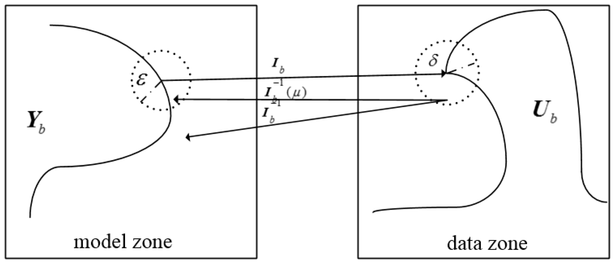
2.2. The Tikhonov Regularization and the L-Curve Method
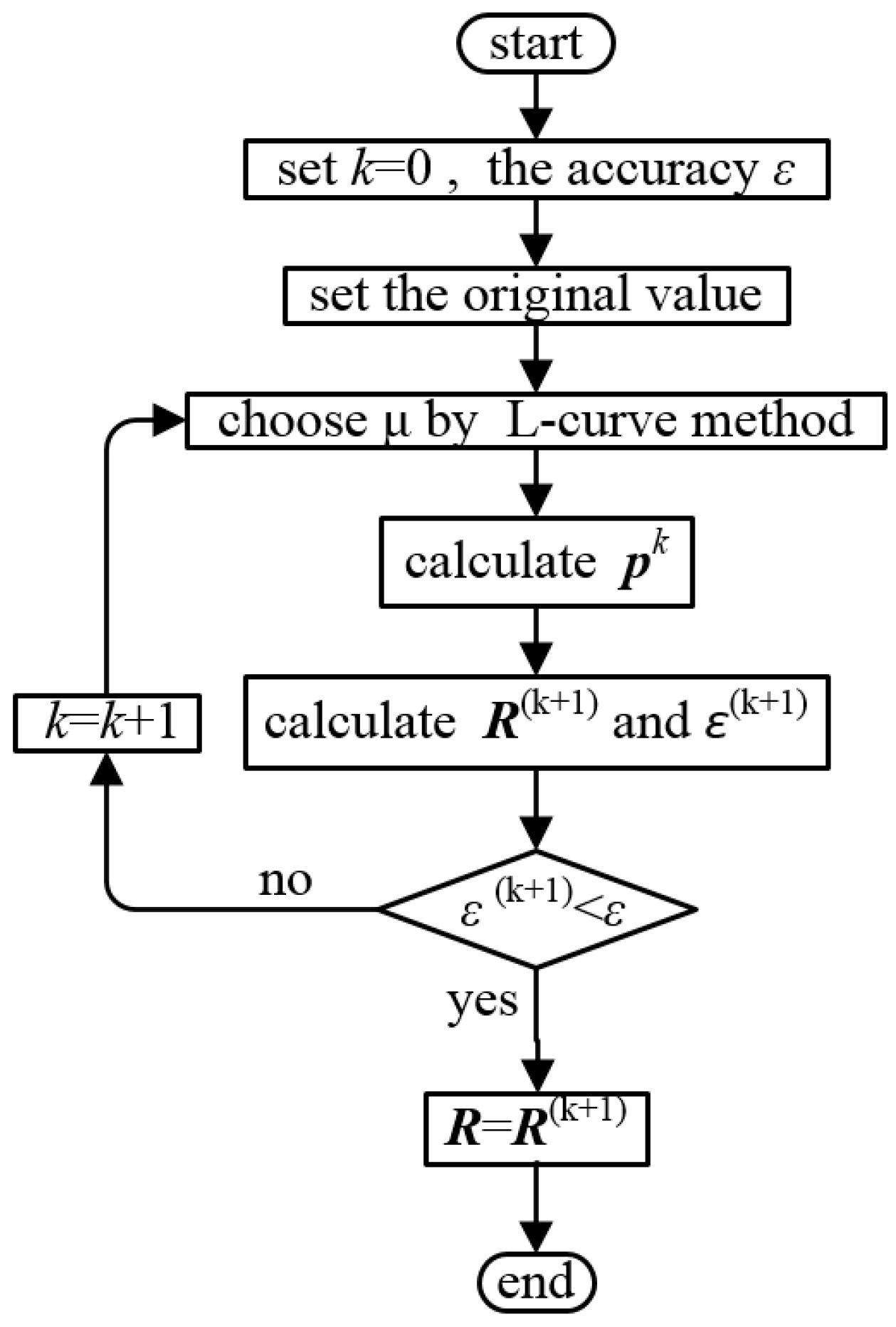
2.3. The Calculation of the Branch Resistance by L-Curve Regularization
- (1)
- Set and the accuracy . The initial value is selected as the branch resistance under normal conditions, .
- (2)
- Calculate the Jacobian matrix and choose the regularization parameter from the L-curve method.
- (3)
- Calculate the iteration step size .
- (4)
- Calculate and the iteration error . If , let ; otherwise, make , and turn towards step (2).
- (5)
- Export the optimal solution .
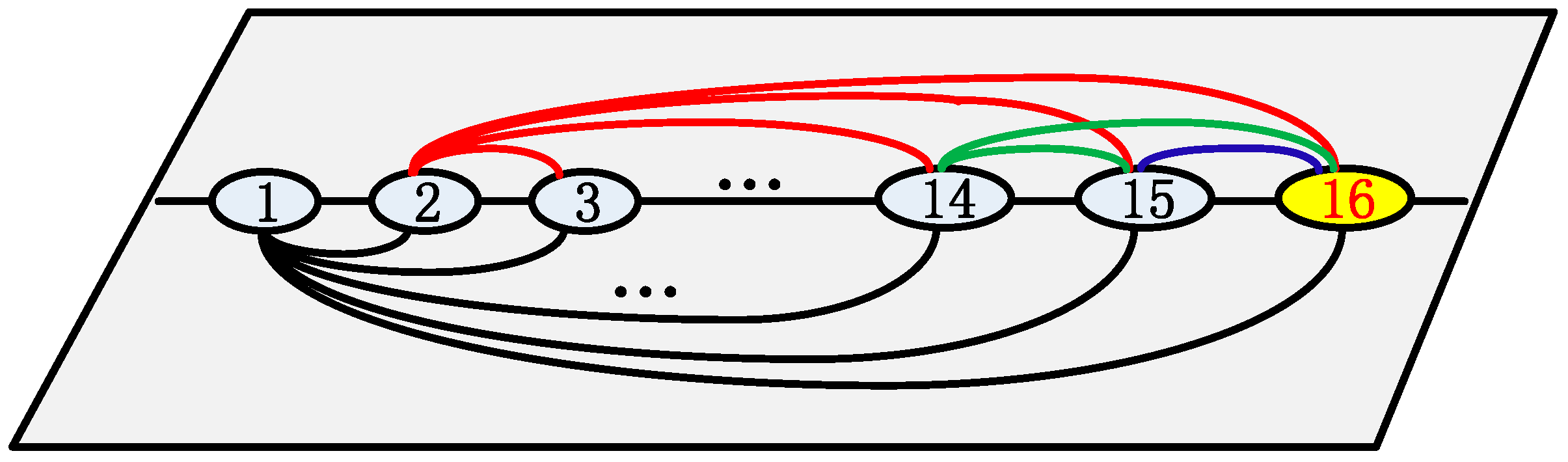
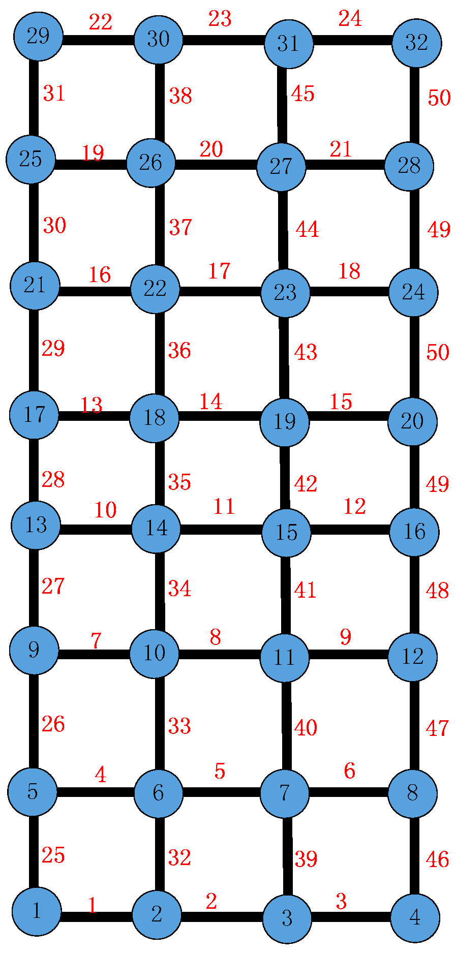
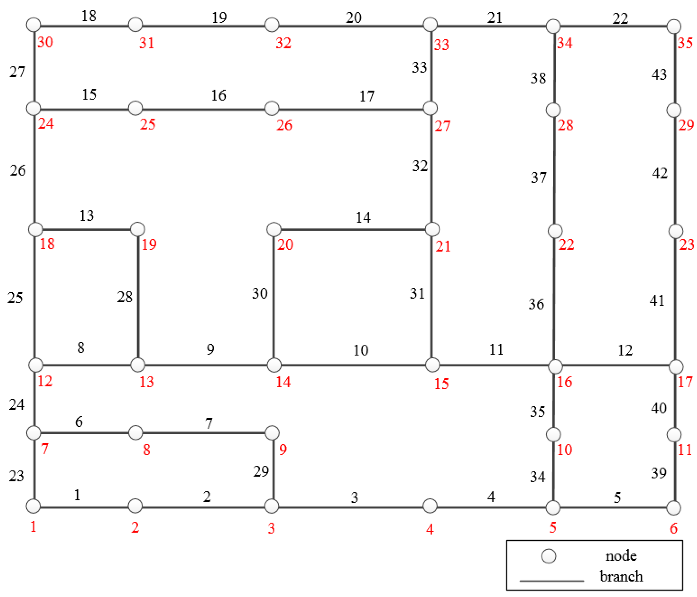
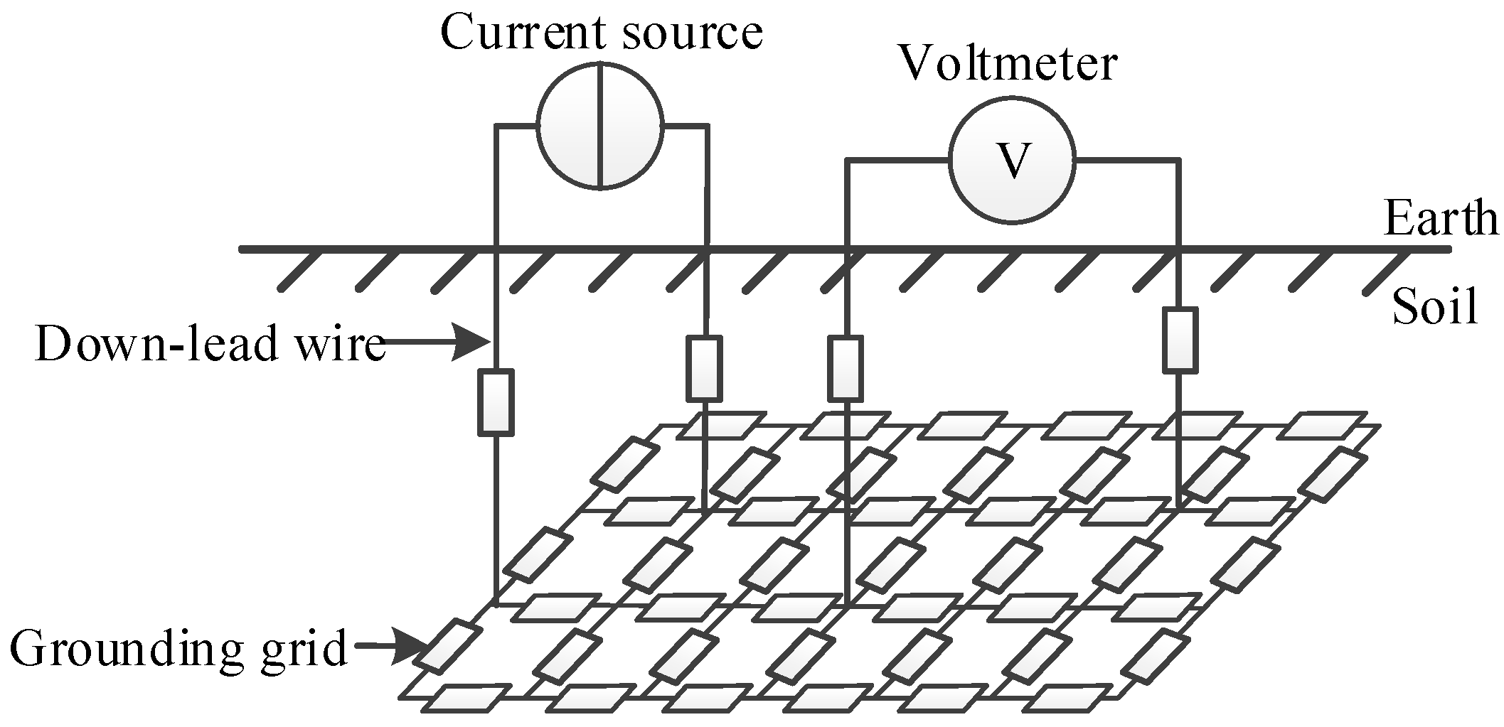
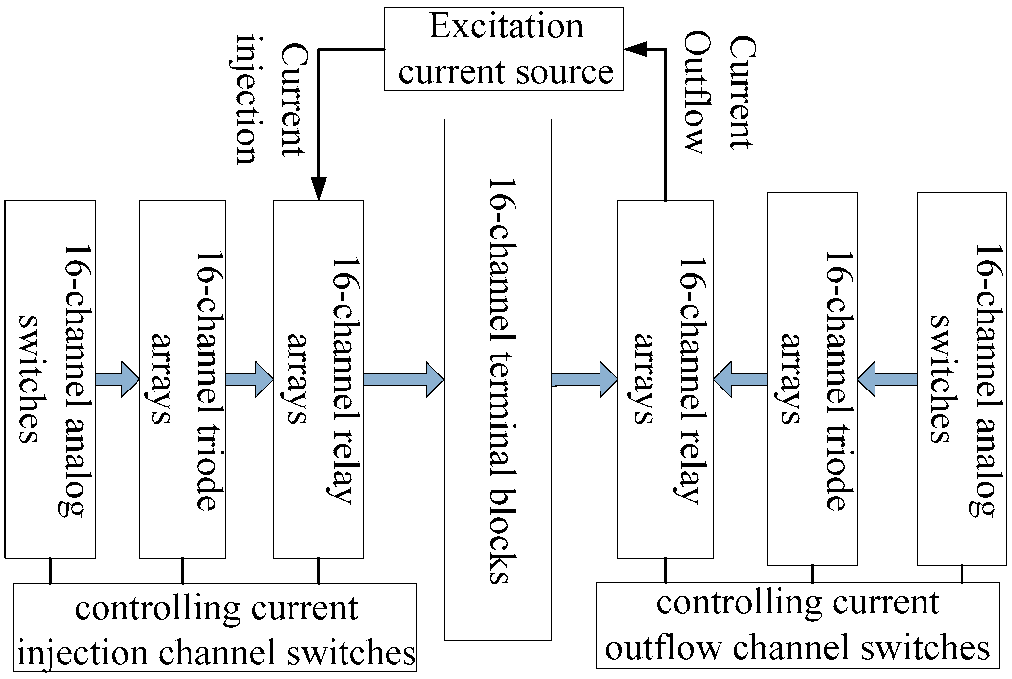
2.4. Principle of Cycle Voltage Measurement
- i = 1, N1 is the outflow node, N2, N3, …, N16 is the inflow node in turn;
- i = 2, N2 is the outflow node, N3, N3, …, N16 is the inflow node in turn;
- ……
- i = 15, N15 is the outflow node, N16 is the inflow node.
3. Experiments and Discussion
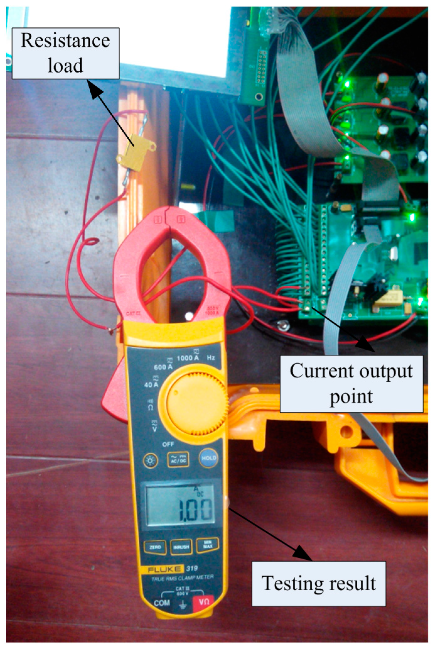
3.1. Lab Tests
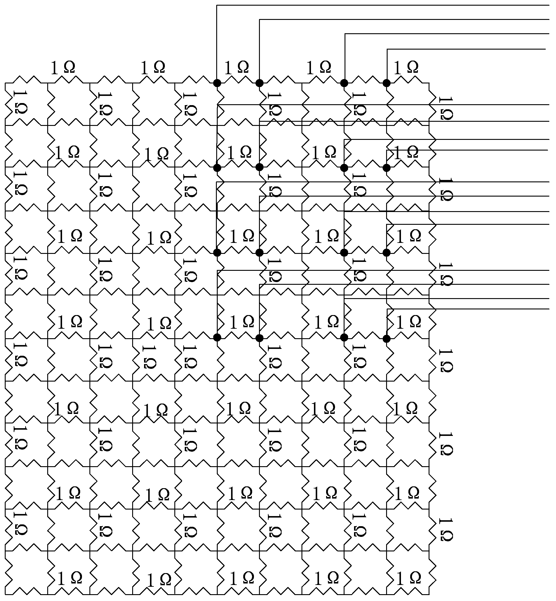
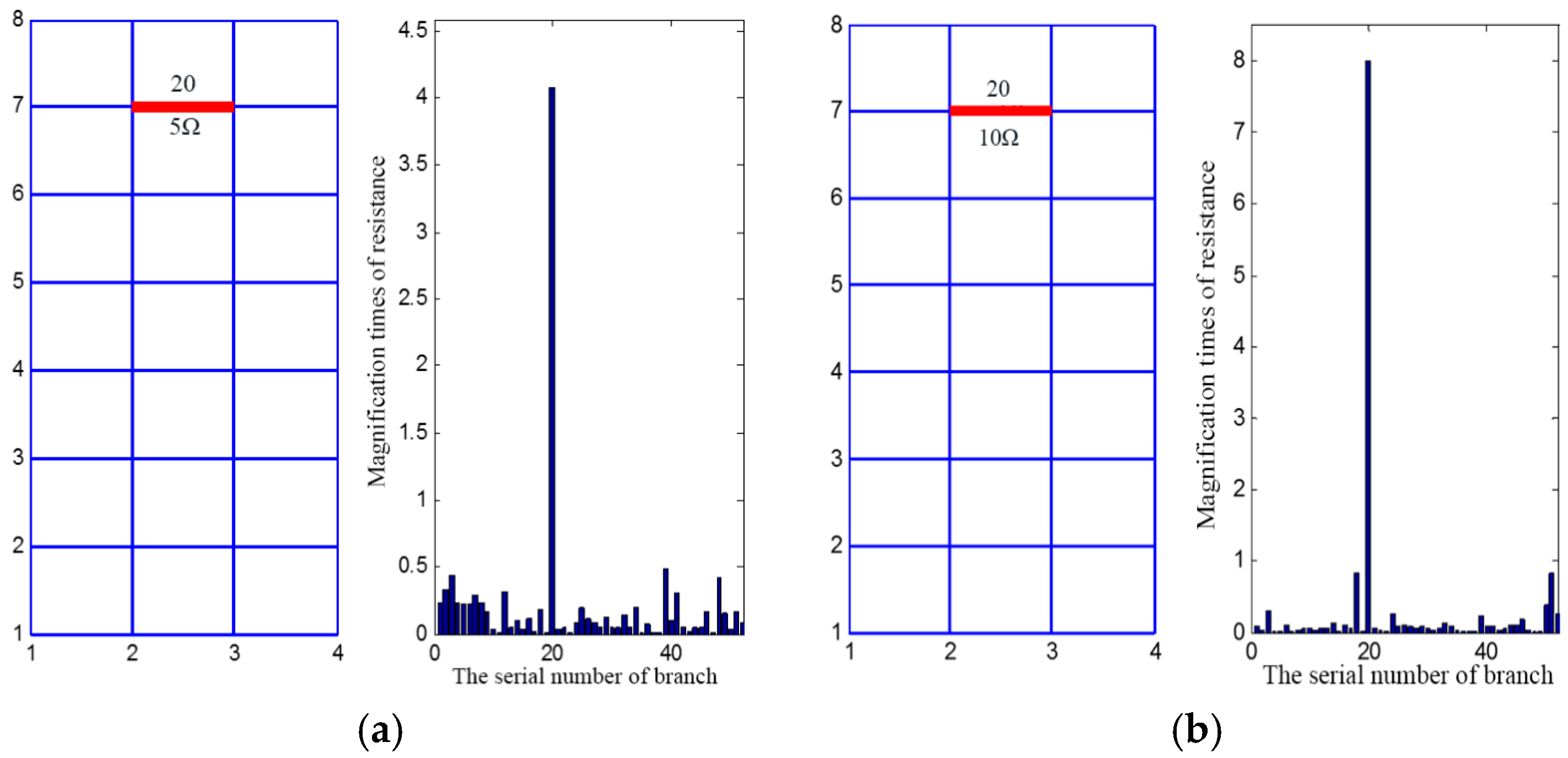
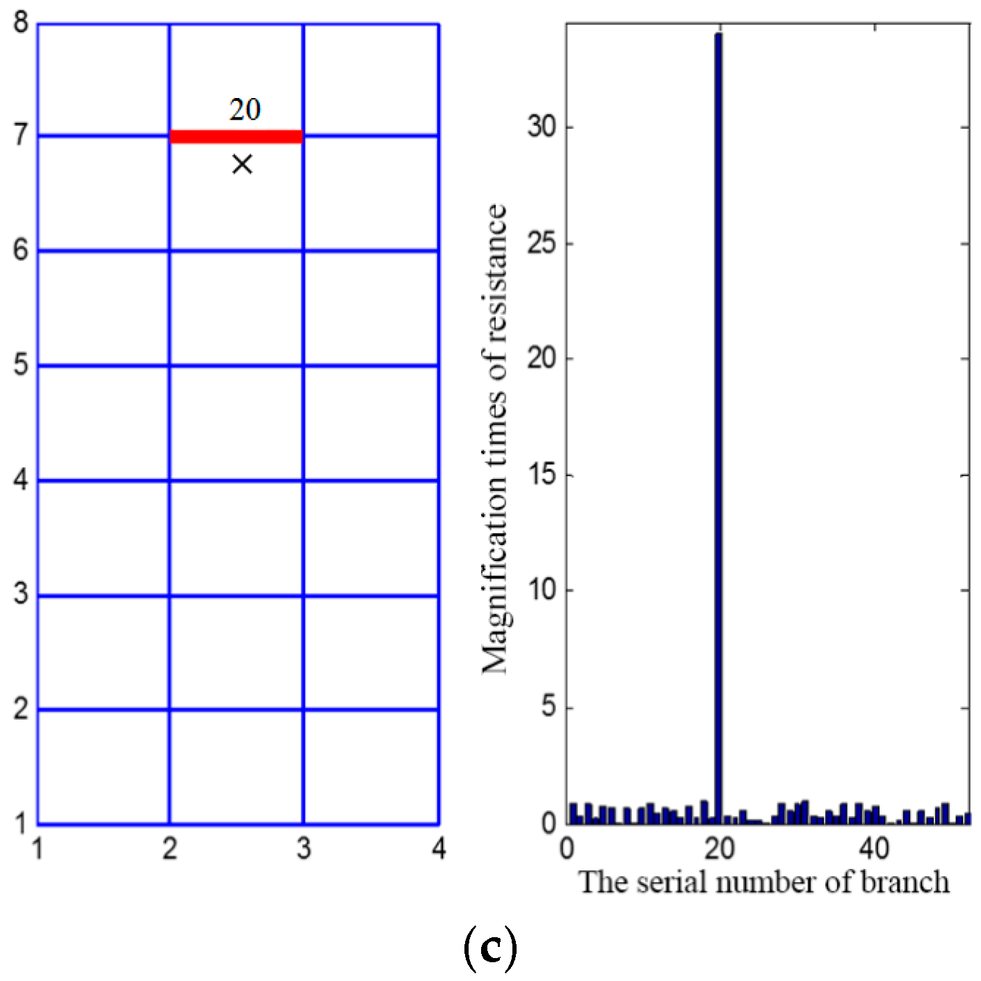
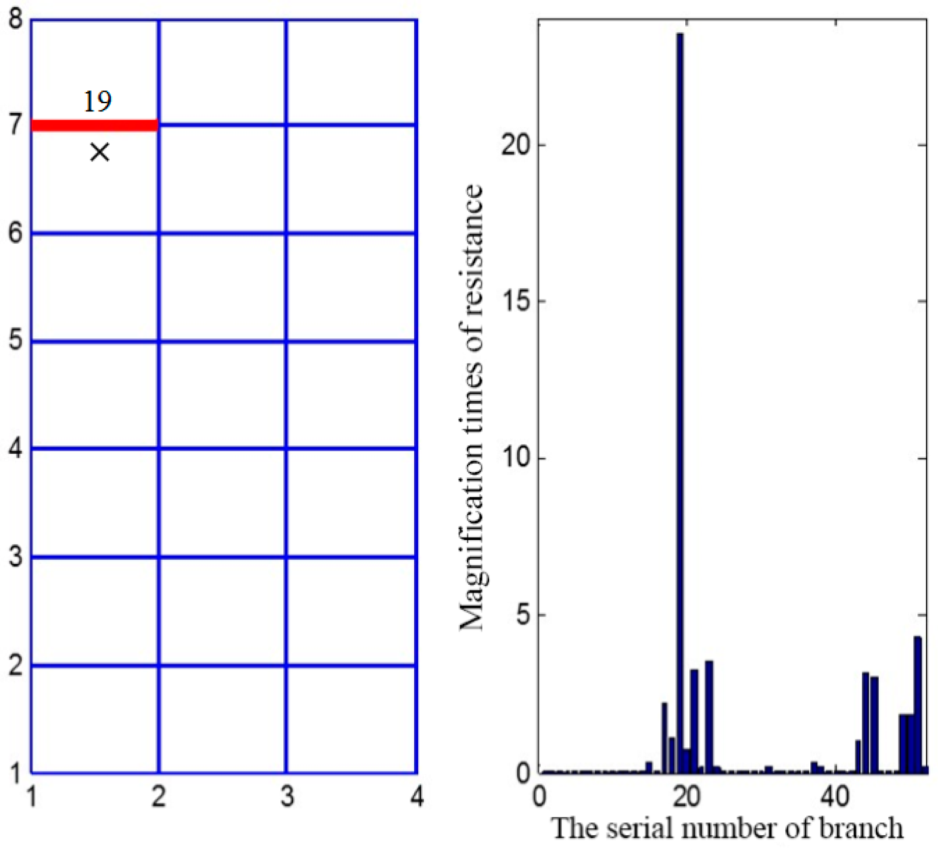
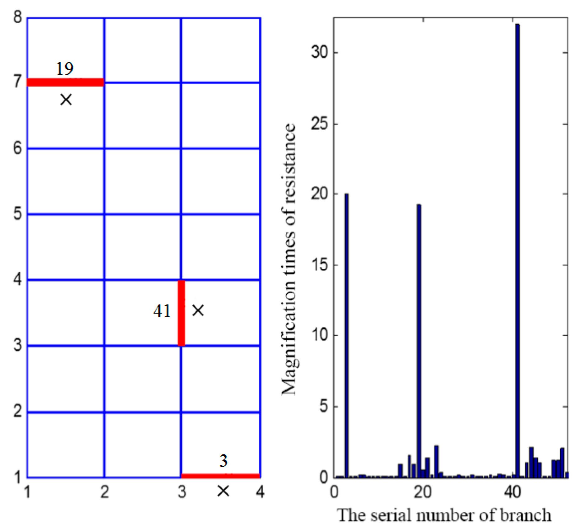
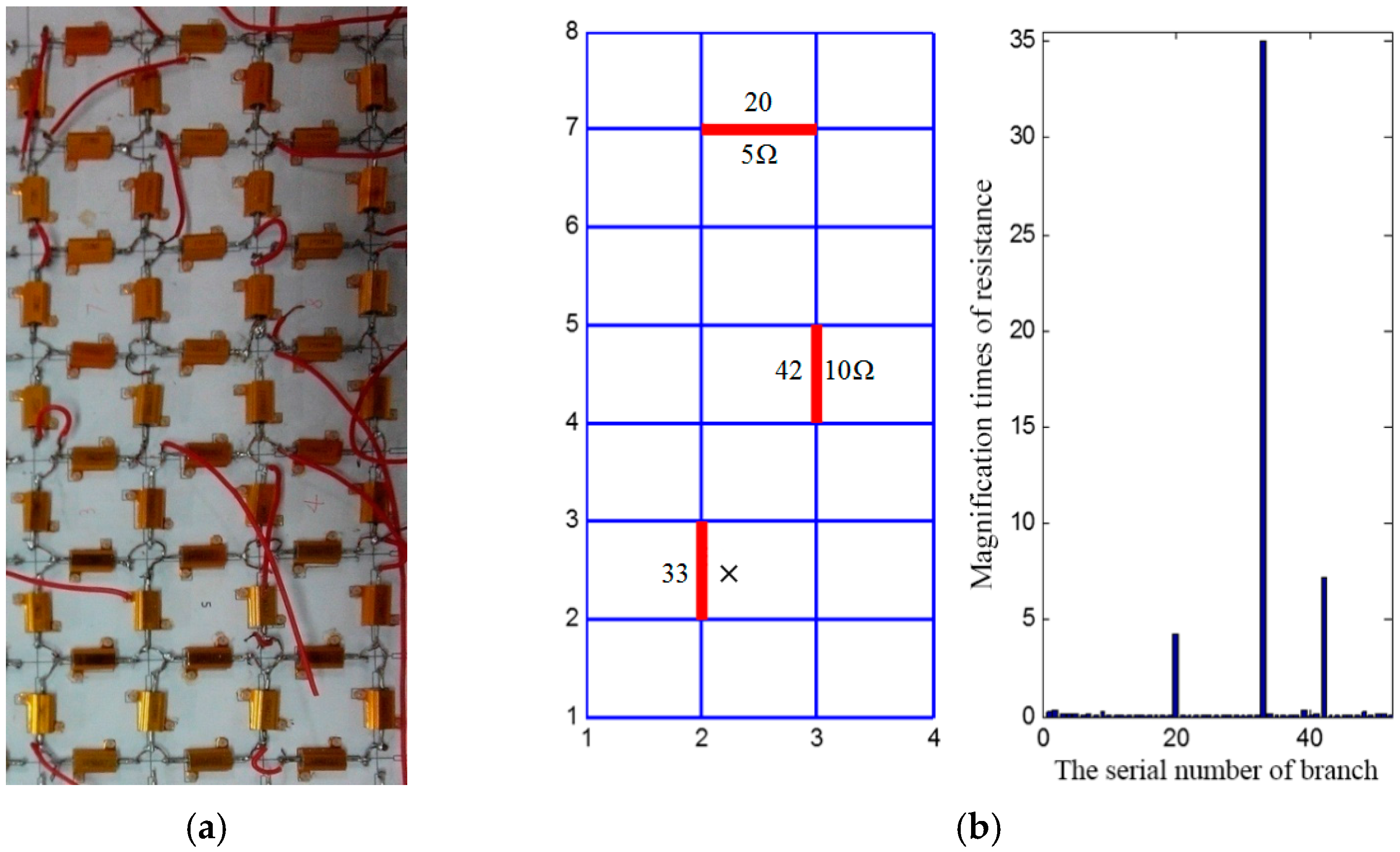
3.1.1. Tests with Precise Resistor
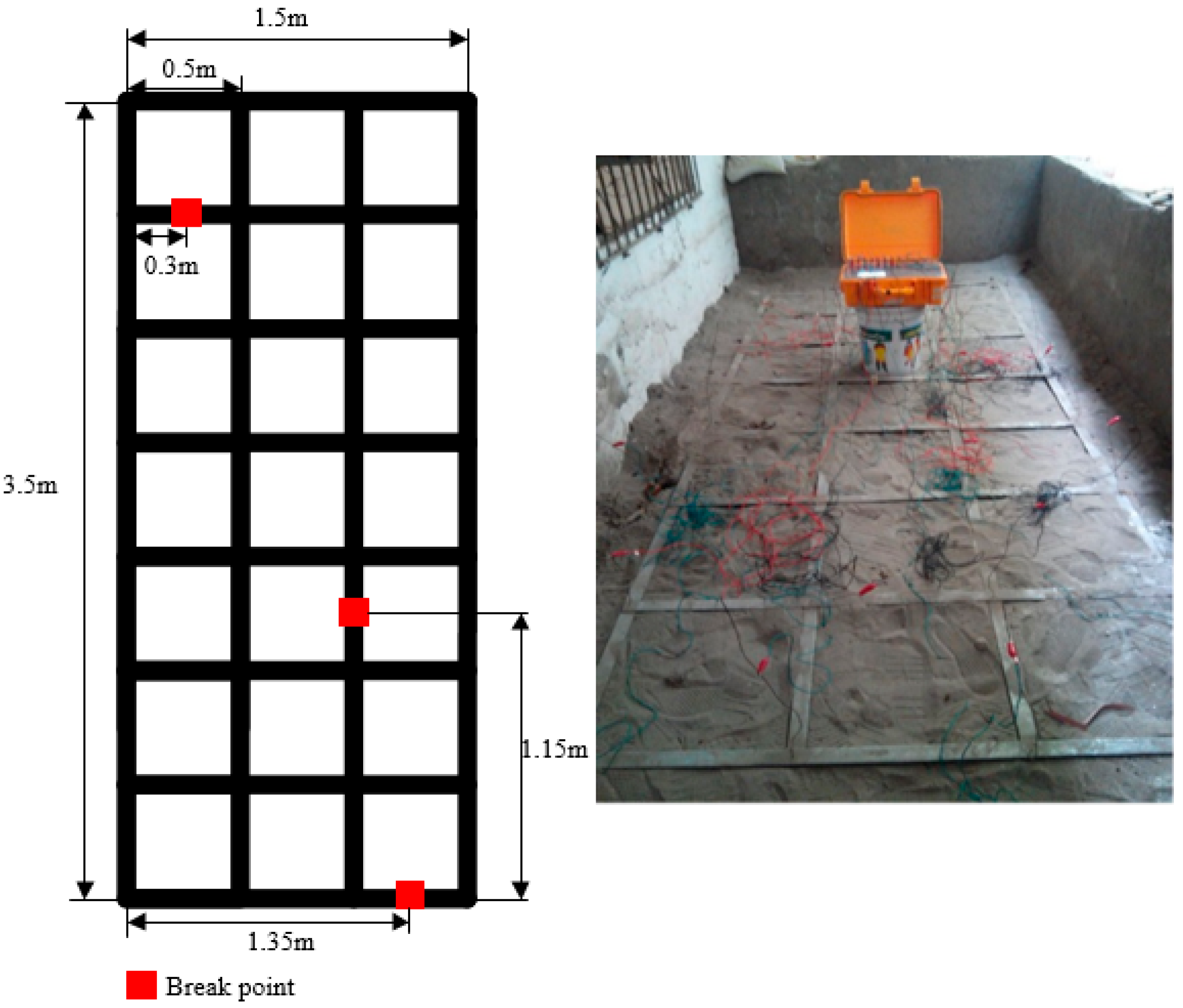
3.1.2. Tests with Galvanized Steel Strap
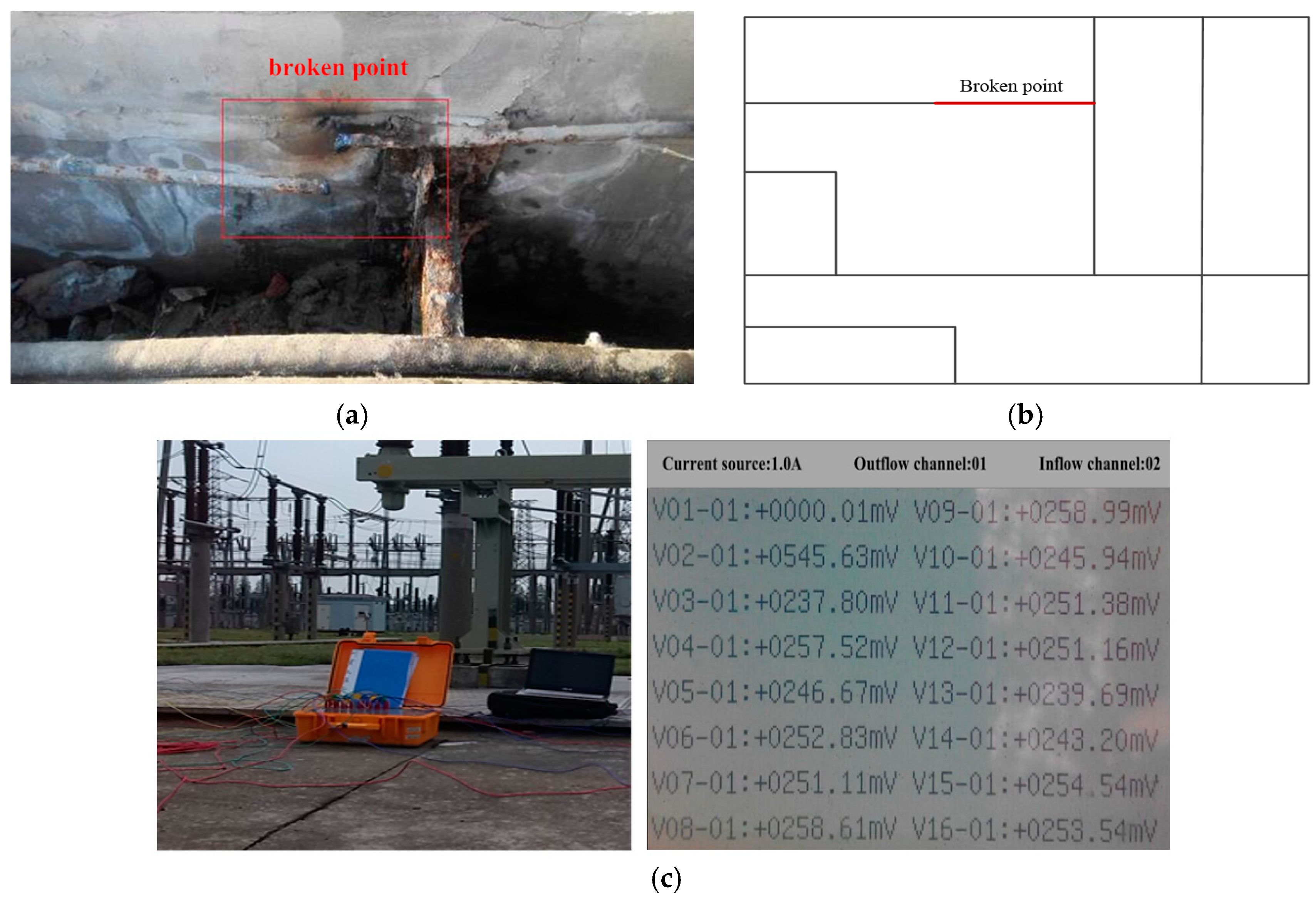
3.2. Field Tests
4. Conclusions
Acknowledgments
Author Contributions
Conflicts of Interest
References
- Asimakopoulou, F.E.; Tsekouras, G.J.; Gonos, I.F.; Stathopulos, I.A. Estimation of seasonal variation of ground resistance using artificial neural networks. Electr. Power Syst. Res. 2013, 94, 113–121. [Google Scholar] [CrossRef]
- Alipio, R.; Schroeder, M.A.O.; Afonso, M.M. Voltage Distribution Along Earth Grounding Grids Subjected to Lightning Currents. IEEE Trans. Ind. Appl. 2015, 51, 4912–4916. [Google Scholar] [CrossRef]
- IEEE PES Substations Committee. IEEE Guide for Safety in AC Substation Grounding; IEEE Standard 80-2000; IEEE: Washington, DC, USA, 2000. [Google Scholar]
- Long, X.; Dong, M.; Xu, W.; Li, Y.W. Online monitoring of substation grounding grid conditions using touch and step voltage sensors. IEEE Trans. Smart Grid 2012, 3, 761–769. [Google Scholar] [CrossRef]
- Kostić, V.I.; Raičević, N.B. A study on high-voltage substation ground grid integrity measurement. Electr. Power Syst. Res. 2016, 131, 31–40. [Google Scholar] [CrossRef]
- Sverak, J.G.; Dick, W.K.; Dodds, T.H.; Heppe, R.H. Safe substation grounding-part I. IEEE Trans. Ind. Appl. 1981, 100, 4281–4290. [Google Scholar] [CrossRef]
- Zhang, X.L.; Luo, P.; Mo, N.; Wang, Y.G.; Li, Y.L. Development and application of electrochemical detection system for grounding grid corrosion state. Proc. CSEE 2008, 28, 152–156. [Google Scholar]
- Dommel, H.W. Digital computer solution of electromagnetic transients in single-and multiphase networks. IEEE Trans. Power Appar. Syst. 1969, PAS-88, 388–399. [Google Scholar] [CrossRef]
- Yu, C.; Fu, Z.; Wang, Q.; Tai, H.M.; Qin, S. A novel method for fault diagnosis of grounding grids. IEEE Trans. Ind. Appl. 2015, 51, 5182–5188. [Google Scholar] [CrossRef]
- Zhang, P.H.; He, J.J.; Zhang, D.D.; Wu, L.M. A fault diagnosis method for substation grounding grid based on the square-wave frequency domain model. Metrol. Meas. Syst. 2012, 19, 63–72. [Google Scholar] [CrossRef]
- Dawalibi, F. Electromagnetic fields generated by overhead and buried short conductors. Part 2—Ground networks. IEEE Power Eng. Rev. 1986, 6, 33–34. [Google Scholar] [CrossRef]
- Heimbach, M.; Grcev, L.D. Grounding system analysis in transients programs applying electromagnetic field approach. IEEE Trans. Power Deliv. 1997, 12, 186–193. [Google Scholar] [CrossRef]
- Zhang, B.; Zhao, Z.; Cui, X.; Li, L. Diagnosis of breaks in substation’s grounding grid by using the electromagnetic method. IEEE Trans. Magn. 2002, 38, 473–476. [Google Scholar] [CrossRef]
- Yang, F.; Jiang, Y.; Shi, Q.; Chen, T.; He, W. Magnetic field inverse problem of grounding grid and its application. Int. J. Appl. Electromagn. 2012, 40, 173–183. [Google Scholar]
- Liu, K.; Yang, F.; Wang, X.; Gao, B.; Kou, X.; Dong, M.; Jadoon, A. A novel resistance network node potential measurement method and application in grounding grids corrosion diagnosis. Prog. Electromagn. Res. M 2016, 52, 9–20. [Google Scholar] [CrossRef]
- Zeng, J.; Lin, S.; Xu, Z. Sparse solution of underdetermined linear equations via adaptively iterative thresholding. Signal Process. 2014, 97, 152–161. [Google Scholar] [CrossRef]
- Liu, J.; Ni, Y.-F.; Lu, W.; Wang, S.; Li, Z.-Z. Influence of touchable nodes deviation on grounding grids corrosion diagnosis and its correction. High Volt. Eng. 2008, 34, 2349–2354. [Google Scholar]
- Wang, X.; He, W.; Yang, F.; Zhu, L.; Liu, X. Topology detection of grounding grids based on derivative method. Trans. China Electrotech. Soc. 2015, 30, 73–78, 89. [Google Scholar]
- Li, C.; He, W.; Yao, D.; Yang, F.; Kou, X.; Wang, X. Topological measurement and characterization of substation grounding grids based on derivative method. Int. J. Electr. Power Energy Syst. 2014, 63, 158–164. [Google Scholar]
- Faleiro, E.; Asensio, G.; Moreno, J. An estimate of the uncertainty in the grounding resistance of electrodes buried in two-layered soils with non-flat surface. Energies 2017, 10, 176. [Google Scholar] [CrossRef]
- Huang, W.; Xiao, L.; Liu, H.; Wei, Z. Hyperspectral imagery super-resolution by compressive sensing inspired dictionary learning and spatial-spectral regularization. Sensors 2015, 15, 2041. [Google Scholar] [CrossRef] [PubMed]
- Li, G.; Li, B.J.; Yu, X.G.; Cheng, C.T. Echo state network with bayesian regularization for forecasting short-term power production of small hydropower plants. Energies 2015, 8, 12228–12241. [Google Scholar] [CrossRef]
- Hanke, M.; Longman Scientific Technical. Conjugate Gradient Type Methods for Ill-Posed Problems; John Wiley & Sons, Inc.: New York, NY, USA, 1995. [Google Scholar]
- Liu, J.; Ni, F.; Wang, Q.; Li, Z.; Wang, S. Grounding grids corrosion diagnosis using a block dividing approach. High Volt. Eng. 2011, 37, 1194–1202. [Google Scholar]


| The Value of Load/Ω | 0.05 | 0.1 | 0.5 | 1.0 | 5.0 | 10.0 | 20.0 | 30.0 | 40.0 |
| The Output Current/A | 1.00 | 1.00 | 1.00 | 1.00 | 1.00 | 1.00 | 1.00 | 0.99 | 0.99 |
| Measured Data by Device (mV) | Simulation Data by MATLAB (mV) | Measurement Error (mV) | Percentage Error (%) |
|---|---|---|---|
| 237.80 | 237.76 | 0.04 | 0.0168% |
| 257.52 | 254.32 | 3.20 | 1.260% |
| 246.67 | 245.10 | 1.57 | 0.641% |
| 252.83 | 252.20 | 0.63 | 0.250% |
| 251.11 | 250.13 | 0.98 | 0.392% |
| 258.61 | 257.92 | 0.69 | 0.268% |
| 258.99 | 256.23 | 2.66 | 1.040% |
| 245.94 | 245.13 | 0.81 | 0.330% |
| 251.38 | 250.63 | 0.75 | 0.300% |
| … | … | … | … |
| Number | 1 | 2 | 3 | 4 | 5 | 6 |
| Inflow Node | 4 | 11 | 6 | 14 | 23 | 30 |
| Outflow Node | 23 | 17 | 28 | 30 | 6 | 17 |
| Number | 1 | 2 | 3 | 4 | 5 | 6 |
| Inflow Node | 2 | 7 | 9 | 18 | 28 | 31 |
| Outflow Node | 28 | 24 | 31 | 28 | 7 | 9 |
© 2017 by the authors. Licensee MDPI, Basel, Switzerland. This article is an open access article distributed under the terms and conditions of the Creative Commons Attribution (CC BY) license (http://creativecommons.org/licenses/by/4.0/).
Share and Cite
Yang, F.; Wang, Y.; Dong, M.; Kou, X.; Yao, D.; Li, X.; Gao, B.; Ullah, I. A Cycle Voltage Measurement Method and Application in Grounding Grids Fault Location. Energies 2017, 10, 1929. https://doi.org/10.3390/en10111929
Yang F, Wang Y, Dong M, Kou X, Yao D, Li X, Gao B, Ullah I. A Cycle Voltage Measurement Method and Application in Grounding Grids Fault Location. Energies. 2017; 10(11):1929. https://doi.org/10.3390/en10111929
Chicago/Turabian StyleYang, Fan, Yongan Wang, Manling Dong, Xiaokuo Kou, Degui Yao, Xing Li, Bing Gao, and Irfan Ullah. 2017. "A Cycle Voltage Measurement Method and Application in Grounding Grids Fault Location" Energies 10, no. 11: 1929. https://doi.org/10.3390/en10111929
APA StyleYang, F., Wang, Y., Dong, M., Kou, X., Yao, D., Li, X., Gao, B., & Ullah, I. (2017). A Cycle Voltage Measurement Method and Application in Grounding Grids Fault Location. Energies, 10(11), 1929. https://doi.org/10.3390/en10111929