Considering Maintenance Cost in Unit Commitment Problems

Abstract

Electric power systems worldwide are receiving an increasing volume of wind power generation (WPG) because of environmental concerns and cost declines associated with technological innovation. To manage the uncertainty of WPG, a system operator must commit sufficient conventional generators to provide an appropriate reserve. At times, frequent start and stop operations are applied to certain generators, which incurs maintenance costs associated with thermal-mechanical fatigue. In this paper, we suggest a comprehensive approach to unit commitment (UC) that considers maintenance cost: the parameters of equivalent start (ES) and equivalent base load hours (EBHs) are adopted in the UC problem to determine optimal generation scheduling. A new formulation for the maintenance cost that can be readily combined with an existing mixed integer linear programming algorithm is presented. The effectiveness of the proposed UC method is verified through simulations based on an IEEE 118-bus test system. The simulation results show that considering maintenance cost in the UC problem effectively restricts frequent start and stop operation scheduling. Furthermore, the operating cost is reduced, the required reserve level is maintained, and the computational time is comparable with that of the conventional UC method.

1. Introduction

In recent years, the installed capacity of wind power generation (WPG) has increased significantly because of environmental concerns. For instance, in the United States, wind energy is expected to provide 15–30% of added power generation by 2024. Tax credits that are available for renewable energy further support the expansion of the wind energy market share [1]. However, the inherent uncertainty and variability of WPG requires a system operator for stable power system operations [2]. One of the fundamental decisions related to the uncertain nature of WPG and load demand is unit commitment (UC), which the system operator assesses one day before the operating day [3]. The purpose of UC is to determine the set of generators that should be run to accommodate available energy and minimize the total operating costs. The UC problem is devised to satisfy both overall system constraints (e.g., power balance between supply and demand, system spinning reserve, and power flow) and unit constraints on each generator (e.g., generator power output, ramp rate, and minimum up and down times).

Although there have been several UC studies that have attempted to utilize demand-side resources [4,5] or wind power itself as a reserve provider [6], the main part of flexibility in power system operation is supplied by a conventional generator. Some generators are scheduled only to meet reserve requirement levels, and these generators are frequently started and stopped, especially during periods of increased variability, resulting in degraded generator performance. To ensure the generator’s efficiency, the generators must be frequently maintained, and therefore, maintenance costs are induced both by the generator’s operation time and by the associated start and stop actions. Reducing these costs is the primary objective of this paper.

Significant attention has been applied to both UC and generator maintenance; however, previous papers did not explicitly address the maintenance costs and production costs at the same time [4,5,6,7,8]. Maintenance scheduling studies focus on determining the timing of maintenance schedules, while weekly average production costs are used for simplicity [9]. On the other hand, for UC studies, the maintenance costs are regarded as fixed [10], or it is assumed that the generator production cost function includes them [11]. The authors of [12] proposed UC considering the maintenance of thermal power system, but they focused on the reliability rather than on economic aspects.

Although frequent start and stop actions and continuous generator operation incur machine malfunctions, which accordingly lead to costs for the system operators, most previous UC models have not considered these influences. This paper proposes an improved UC model that reflects generator deterioration as maintenance costs and determines the optimal long-term generation schedule that minimizes total generation and maintenance costs. The model adopts the parameters of equivalent start (ES) and equivalent base load hour (EBH) to accurately calculate the maintenance costs. The ES is adopted to evaluate the on–off action of the peak load generators, which usually operate on daily start and stop schedules. The EBH is implemented to calculate the maintenance costs associated with the operation time of the base load generators, which operate on weekly start and stop schedules.

Since various power system constraints and individual generator limits impact the UC optimization problem, a technique to attack the problem is highly important. Today’s significantly expanded power systems rely on a rapid convergence to reduce computational time. Various techniques have been applied to the UC problem, including dynamic programming (DP) [13], priority-list [14], Lagrange relaxation [15], and mixed integer linear programming (MILP) [16]. Among these techniques, MILP has been favorably adopted in many market operators in the United States because MILP approaches are more capable of accommodating integer variables to determine optimal solutions [17]. To further enhance the utility of the existing MILP algorithm, we present a new mathematical formulation of the relevant maintenance costs. Maintenance costs associated with both ES and EBH are expressed as integer variables and linearized, and the computational times measured in simulations verify that this procedure efficiently determines the optimal solution.

The remainder of this paper is organized as follows. Section 2 describes the modeling of maintenance costs, including the ES and EBH formulations. Section 3 presents the method for formulating the UC with maintenance costs. The performance of the proposed method is evaluated in Section 4 through simulations results obtained using IEEE 118-bus test systems. Finally, Section 5 summarizes our conclusions.

2. Modeling of ES and EBH

To precisely model the maintenance cost, we classified each generator as either a peak load generator or a base load generator. ES is the parameter to determine maintenance costs of a peak load generator, whereas EBH is related to a base load generator. Before calculating the maintenance costs, ES and EBH should be expressed in a MILP form.

2.1. ES Modeling for Peak Load Generators

Maintenance costs associated with peak load generators are mainly due to their rapid start and stop operations. Daily start and stop operations place thermal-mechanical stress on the generator, reducing its life expectancy. When the cumulative total number of ESs reaches the contracted value, the system operator should shut off the generator until the machine can be inspected and repaired. The ES value of peak load unit $p$ that can have several loading levels at time $t$ can be expressed as

$$E{S}_t^p={\displaystyle \sum _{k=1}^{N{L}_p}{W}_k^p{X}_{t,k}^p}$$

(1)

$${\displaystyle \sum _{k=1}^{N{L}_p}{X}_{t,k}^p}=D_{t+1}^p$$

(2)

$$S_t^p-D_t^p=U_t^p-U_{t-1}^p$$

(3)

$$S_t^p+D_t^p\le 1$$

(4)

$$P_t^p={\displaystyle \sum _{k=1}^{N{L}_p}{\mathrm{Limit}}_k\cdot X_{t,k}^p}+{\delta }_t^p+{\delta }_t^{\prime p}$$

(5)

$$0\le {\delta }_t^p\le {\mathrm{Limit}}_{k+1}-{\mathrm{Limit}}_k$$

(6)

$$0\le {\delta }_t^{\prime p}\le P_{\max }^p\cdot (1-D_{t+1}^p).$$

(7)

In Equation (1), $X_{t,k}^p$ is multiplied by the weighting factor $W_k^p$ for output block $k$, set in accordance with the loading level of the unit to reflect the fact that a generator endures significant stress when it shuts off under a high loading condition. Here, $X_{t,k}^p$ is a binary variable that indicates the $k$-th loading level on unit $p$ at time $t$ (that is, if the generator has an output between ${\mathrm{Limit}}_k$ and ${\mathrm{Limit}}_{k+1}$ at time $t$ and shuts down at time $t+1$, the value of $X_{t,k}^p$ becomes 1). ${\mathrm{Limit}}_k$ denotes the start or end point of a block of the generated power output. Equation (2) expresses that only one of the $X_{t,k}^p$ values can equal 1 when the generator shuts off at next time $t+1$. In other words, only one $X_{t,k}^p$ can be 1 in each hour $t$, whereas all the other $X_{t,k}^p$ remain 0 over that time. $D_t^i$ and $S_t^i$ indicate whether the generator’s status has changed into the off and on states from the on and off states, respectively. These variables are binary values that cannot both be 1 at the same time, as shown by (3) and (4).

$P_t^p$ represents the output of the peak generator, as determined using Equations (5)–(7). If the generator is scheduled to be off at time $t+1$, the output of the generator at time $t$, $P_t^i$ is decided by ${\delta }_t^p$ in Equation (5) and $X_{t,1}^p$ through $X_{t,N{L}_p}^p$. When the generator is continually on, $\delta {\prime }_t^p$ results in a $P_t^p$ value that is between its minimum and maximum constraints. This is represented as Equation (7). For example, a generator with $P_{\min }^p={\mathrm{Limit}}_1=20\mathrm{MW}$, ${\mathrm{Limit}}_2=40\mathrm{MW}$, ${\mathrm{Limit}}_3=60\mathrm{MW}$, and ${\mathrm{Limit}}_{N{L}_p}{=\mathrm{Limit}}_4=80\mathrm{MW}$ turns off after consuming 45 MW; in this case, $X_{t,2}^p$ becomes 1, and ${\delta }_t^p$ takes the value 5 MW, while $X_{t,1}^p$, $X_{t,3}^p$, and $X_{t,4}^p$ are all 0. On the other hand, if the output power of the generator is maintained 45 MW at $t+1$, all the $X_{t,k}^p$ are 0, and ${\delta }_t^{\prime p}$ results in 45 MW. Through Equations (1)–(7), the ES is calculated according to the respective loading levels only when the relevant generator is shut down.

2.2. EBH Modeling for Base Load Generators

The EBH related to the base load generators is calculated by assessing the duration of each machine’s operation. In general, base load generators do not frequently switch on and off; instead, they run for at least for a week or up to several weeks. Therefore, their maintenance schedules are mainly determined by their operation times rather than their on–off actions.

The EBH is formulated to reflect how long the generator operates and under what condition. As in the peak load generator case, a system operator should shut down the generator for maintenance when the cumulative total EBH operation time reaches a predetermined value. The EBH’s unit is the hour, whereas the ES’s unit is the number of switching times. Because generators are usually stressed when the output exceeds the base load limit, the EBH value of base load unit $b$ at time $t$ can be expressed as

$$EB{H}_t^b=T{W}_1^{b}TL{X}_t^b+T{W}_2^{b}TU{X}_t^b$$

(8)

$$TL{X}_t^b+TU{X}_t^b=U_t^b$$

(9)

$$P_t^b=P_{\min }^b\cdot TL{X}_t^b+{\mathrm{Baseload}\mathrm{Limit}}_b\cdot TU{X}_t^b+{\delta }_t^b$$

(10)

$$0\le {\delta }_t^b\le {\mathrm{Baseload}\mathrm{Limit}}_b-P_{\min }^b.$$

(11)

The overall EBH modeling procedure is analogous to that of the peak load generator except that there is only one division in the loading condition: $U_t^b$ indicates that the generator is committed on the system at time $t$, $TLX$ and $TUX$ are only counted when the generator output is under or over the base load limit, respectively, and $T{W}_1^b$ and $T{W}_2^b$ represent the weighting factors for $TLX$ and $TUX$, respectively.

Because base load generators suffer from higher thermal-mechanical fatigue when they run beyond the base load condition, the $T{W}_2^b$ contribution of that unit to EBH is set to be larger than the $T{W}_1^b$ of the unit that operates below the base load condition. Note that the duration over which the generators are on is important, the last term of Equation (9) is $U_t^b$, rather than this variable’s counterpart in Equation (2), which is $D_t^i$. The output of the base load generator is analogously determined to be between its minimum and maximum values through Equations (10) and (11).

3. UC Formulation with Maintenance Cost

3.1. Maintenance Cost Calculation

The system operator should execute maintenance on the generator to sustain its function and guarantee its rated lifespan whenever either the cumulative ES or the cumulative EBH reaches a specific predetermined value. Each maintenance event costs the Contracted Maintenance Price (CMP), and the unit maintenance costs ($MCOS{T}_{ES}^p$ or $MCOS{T}_{EBH}^b$) can be calculated as follows.

$$MCOS{T}_{ES}^p=\frac{\mathrm{CMP}}{\mathrm{Contracted}\mathrm{ES}\mathrm{for}\mathrm{Generator}p}$$

(12)

$$MCOS{T}_{EBH}^b=\frac{\mathrm{CMP}}{\mathrm{Contracted}\mathrm{EBH}\mathrm{for}\mathrm{Generator}b}.$$

(13)

Naturally, the operation of each generator $p$ or $b$ according to time $t$ entails an additional maintenance cost, as expressed in Equations (19) and (20).

$$C_M^p=E{S}_t^p\cdot MCOS{T}_{p,ES}$$

(14)

$$C_M^b=EB{H}_t^b\cdot MCOS{T}_{b,EBH}.$$

(15)

$MCOS{T}_{ES}^p$ and $MCOS{T}_{EBH}^b$ are expressed in units of $/number of times and $/hour, respectively; hence, both $C_M^p$ and $C_M^b$ have the unit $. The form represented by $C_M^p$ and $C_M^b$ rather than $MCOS{T}_{ES}^p$ and $MCOS{T}_{EBH}^b$ enables the maintenance cost to be simply added to the objective function of the UC optimization problem.

3.2. UC Formulation with Maintenance Cost

The overall UC formulation with the added maintenance cost includes the objective function, Equation (16), and the constraints, Equations (20)–(35).

3.2.1. Objective Function

$$\underset{U,P}{\min }\left\{\begin{array}{l}{\displaystyle \sum _{t=1}^T{\displaystyle \sum _{i=1}^N\left\{C_G^i(P_t^i,U_t^i)+C_{SU}^i(U_t^i)+C_{SD}^i(U_t^i)\right\}}}+\\ {\displaystyle \sum _{t=1}^T{\displaystyle \sum _{p=1}^{NP}\left\{C_M^p(P_t^p,U_t^p)\right\}}}+{\displaystyle \sum _{t=1}^T{\displaystyle \sum _{b=1}^{NB}\left\{C_M^b(P_t^b,U_t^b)\right\}}}\end{array}\right\}$$

(16)

$$C_G^i(P_t^i,U_t^i)=a^i\cdot U_t^i+b^i\cdot P_t^i$$

(17)

$$C_{SU}^i(P_t^i,U_t^i)=K_{SU}^i\cdot (U_t^i-U_{t-1}^i)$$

(18)

$$C_{SD}^i(P_t^i,U_t^i)=K_{SD}^i\cdot (U_{t-1}^i-U_t^i).$$

(19)

The objective function of the problem aims to minimize the total operating cost, constituted by production, startup, shutdown, and maintenance costs, as shown in Equation (16). For simplicity, the production costs function, Equation (17), is expressed as a linear function. If the production costs function is a quadratic function, it can be precisely approximated using a piecewise linearization. The startup cost and shutdown costs are formulated as Equations (18) and (19), respectively.

3.2.2. Constraints

$$P{G}_t^n-P{D}_t^n={\displaystyle \sum _{l=1}^{L^n}{F}_t^l}$$

(20)

$$P{G}_t^n={\displaystyle \sum _{i=1}^{G^n}{P}_t^i}+P_t^{wind,n}$$

(21)

$$U_t^i\cdot P_{\min }^i\le P_t^i\le U_t^i\cdot P_{\max }^i$$

(22)

$$S{R}_t\le {\displaystyle \sum _{i=1}^{N}P{R}_t^i}$$

(23)

$$P{R}_t^i\le P_{\max }^i-P_t^i$$

(24)

$$P{R}_t^i\le R{C}^i\cdot T_{\mathrm{lead}}$$

(25)

$$P_t^i-P_{t-1}^i\le [1-U_t^i\cdot (1-U_{t-1}^i)]\cdot R{C}^i+U_t^i\cdot (1-U_{t-1}^i)\cdot P_{\min }^i$$

(26)

$$P_{t-1}^i-P_t^i\le [1-U_{t-1}^i\cdot (1-U_t^i)]\cdot R{C}^i+U_{t-1}^i\cdot (1-U_t^i)\cdot P_{\min }^i$$

(27)

$${\displaystyle \sum _{t=1}^{G^i}(1-U_t^i)}=0$$

(28)

$${\displaystyle \sum _{n=t}^{t+U{T}^i-1}{U}_t^i}\ge U{T}^i\cdot (U_t^i-U_{t-1}^i)$$

(29)

$${\displaystyle \sum _{n=t}^T[U_n^i-(U_t^i-U_{t-1}^i)]}\ge 0$$

(30)

$${\displaystyle \sum _{t=1}^{L^i}{U}_t^i}=0$$

(31)

$${\displaystyle \sum _{n=t}^{t+D{T}^i-1}(1-U_t^i)}\ge D{T}^i\cdot (U_{t-1}^i-U_t^i)$$

(32)

$${\displaystyle \sum _{n=t}^T[1-U_n^i-(U_{t-1}^i-U_t^i)]}\ge 0$$

(33)

$$F_t^l=\frac{1}{X^l}({\theta }_t^{l,s}-{\theta }_t^{l,r})$$

(34)

$$-F_{\max }^l\le F_t^l\le F_{\max }^l.$$

(35)

Same constraints as Equations (1)–(11).

(36)

Equations (20), (21), and (34) represent the DC power flow equations. Generation limits of thermal generators are stated in (22). The constraints, Equations (23)–(25), are related to the spinning reserve. The spinning reserve, which can be provided by generating units, are constrained by their maximum available power, Equation (23), and by their ramping capability, Equation (24). The ramp up/down limit for the generating units are expressed as Equations (26) and (27), respectively. The minimum up/down time constraints are shown in Equations (28)–(30) and Equations (31)–(33). Because the initial/final status of the generating units should be considered additionally, minimum up time constraints are formulated by three separate equations. The consideration of a minimum down time can be taken into account in the same way as well. Transmission flow limits are set as Equation (35). A more detailed description of the equations can be found in [4,18].

4. Numerical Results

In this section, the proposed method was applied to a practical problem based on the IEEE 118-bus test system, which consists of 118 buses, 91 load sides, 54 generating units, and 186 transmission lines; specifications of the relevant facilities can be found in [19]. There are various types of generating units in the system. Most peak generators have a minimum power output of 5 MW (maximum of 20 MW), and the base load generators usually have a minimum power output of 100 MW (maximum of 300 MW). It was assumed that the total installed wind capacity was 3000 MW, and the wind farms were located at Bus No. 15, 54, and 80. The proportions of the wind farms were set at 50%, 30%, and 20% for each bus, respectively. We solved the UC problem with a 24 h scheduling horizon.

The forecasted demand and WPG are listed in

Table 1. Forecasted demand and wind power generation (WPG) values.

Time (h)	1	2	3	4	5	6	7	8	9	10	11	12
Demand (MW)	4200	3960	3480	2400	3000	3600	4200	4680	4920	5280	5340	5040
WPG (MW)	600	585	615	630	570	555	570	585	525	495	510	585
Time (h)	13	14	15	16	17	18	19	20	21	22	23	24
Demand (MW)	4800	4560	5280	5400	5100	5340	5640	5880	6000	5400	5220	4920
WPG (MW)	615	645	615	570	525	480	450	435	480	510	525	495

, with WPG data taken from [20]. The wind energy penetration level of the WPG data is 11.6%. The required volume of the spinning reserve was set to be three and a half times the standard deviation of the net load forecasting error [21]. For simplicity, network constraints were formulated based on the DC power flow equations, and only the power flow was considered [22]. The maintenance cost of a generating unit obviously varies for different machine manufacturers and maintenance contracts. Therefore, we simulated different maintenance costs based on case studies presented in [23], in which extensive maintenance cost investigations are summarized.

The UC problems were solved using Xpress-mp 64-bit software on a PC with a 2.30-GHz Intel^® Core i5 CPU. The relative dual gap of the problem was set to 0.1%.

First, the total operating costs incurred by the proposed method were compared to those of the conventional method to confirm the cost savings that could be gained with the proposed method. The conventional method indicates that the UC problem is optimized only with the consideration of the generation cost, not with the consideration of the maintenance cost. The maintenance cost of the conventional method is calculated based on the results of the solved UC problem. For this purpose, the maintenance contract cost was set to $1.54 million per maintenance procedure, which is a common standard cost incurred by Korean power companies. As indicated by the results presented in

Table 2. Total operating costs (CMP = $1.54 million) of both methods.

Classification	Proposed Method	Conventional Method
Generation cost (thousand $)	1435.69	1429.82
Maintenance cost (thousand $)	50.47	87.34
Total cost (thousand $)	1486.16	1517.16
Cost savings (thousand $)	31.00 (2.09%)

, cost savings can be achieved by considering the maintenance cost in the UC calculation. The table also shows that generation costs related to energy production increased slightly because the combination of committed generators was altered compared to that implemented with the conventional method. However, this adjustment resulted in a significant decrease in the maintenance cost, which was more than sufficient to compensate for the increased generation costs.

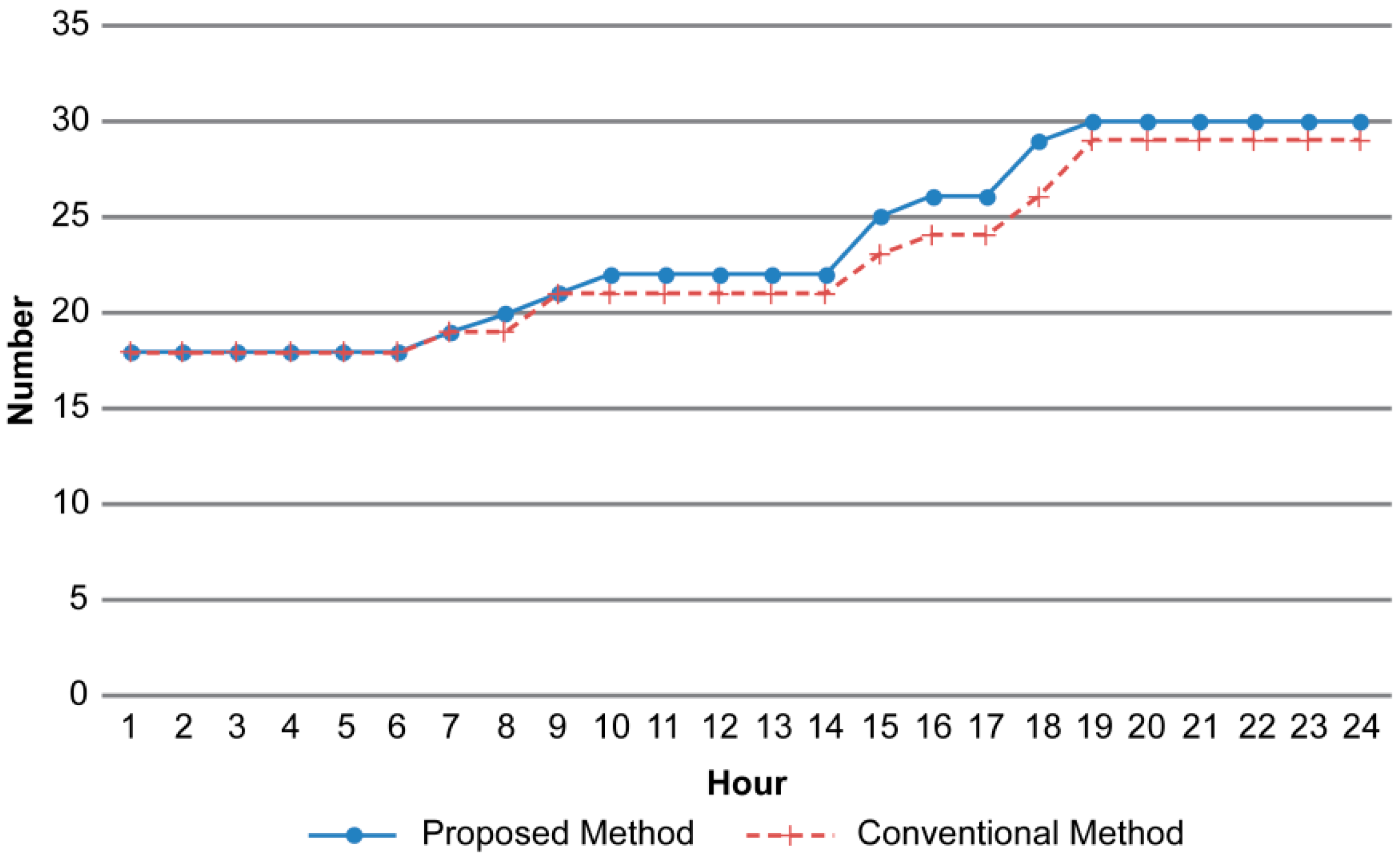
We then compared the UC results. The number of generators online in every hour is presented in Figure 1. The total number of online generators increased when the maintenance cost was considered in the UC process, even though maintenance costs incur when generators are turned on. This result is considered reasonable because the maintenance costs are not only affected by the switching operations, but also by the generating loading level that is determined by the system operator.

To further investigate the maintenance cost, we compared the EBH values of the two approaches for the given scheduling horizon, as shown in

Table 3. Equivalent base load hours of both methods.

Classification	Proposed Method	Conventional Method
EBH (hours)	408	706

. The ES values were not compared because the two methods produced almost the same values. A more significant difference between the ES values is expected to arise with greater WPG penetration levels.

The lower EBH resulting from the proposed method generates significant cost savings. To avoid excessive maintenance costs, the system operator adjusts the power output of some generators to be below the base load limit.

Table 4. Hourly dispatched volume of Generator No. 29.

Hour (h)	Conventional Method	Proposed Method
	Dispatched Volume (MW)	Dispatched Volume (MW)
19	278	267
20	285	289
21	285	289
22	256	256
23	245	234
24	223	223

presents the hourly dispatch volume of the No. 29 generator, for which the base load limit was set at 285 MW. With the conventional method, the No. 29 generator’s output exceeded the base load limit in Hours 20 and 21, whereas with the proposed method, this generator’s output did not exceed the limit. Hence, the maintenance costs associated with this generator can be reduced.

The performance of the proposed method was also evaluated based on different CMPs. In contrast with the previous simulation, in which the CMP was selected based on Korean standards, we set the CMP at $5.25 million for the major maintenance interval, as per [23]. The maintenance cost specified in [23] is calculated by averaging the maintenance cost of complete intervals, just as the Korean standard CMP is determined. The costs take into account of inspecting combustion and the gas path. The primary reason for the different CMPs of the Korean case and that presented in [23] is the different dates on which the costs were estimated. The Korean CMP was calculated based on a fairly up-do-date inspection method. The impacts of different CMPs on the operating costs are summarized in

Table 5. Total operating costs (CMP = $5.25 million) of both methods.

Classification	Proposed Method	Conventional Method
Generation cost (thousand $)	1444.09	1429.82
Maintenance cost (thousand $)	157.92	296.52
Total cost (thousand $)	1602.01	1726.34
Cost savings (thousand $)	124.33 (7.76%)

.

As in the previous simulation based on the Korean CMP, the total operating cost is shown to be reduced with the proposed method. The results show larger cost savings compared to the Korean CMP case, where the CMP was relatively low and resulted in a conservative result.

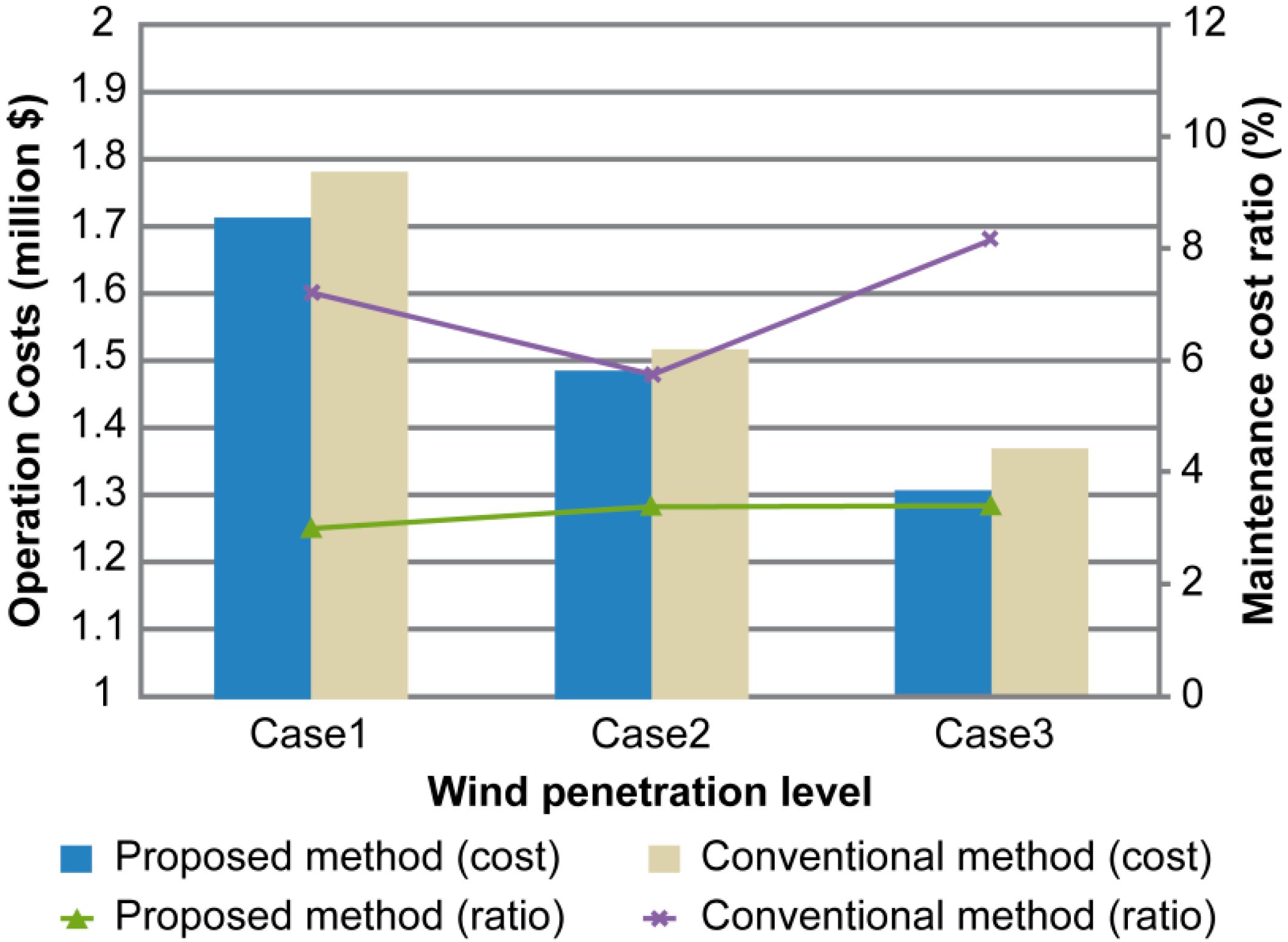
In Figure 2, the performance of the proposed method is illustrated with different wind penetration levels in the power system. The maintenance cost ratio means the ratio of maintenance costs to operating costs. Case 2 is the reference case that we performed previously, whereas Case 1 and Case 3, compared with Case 2, represent 50% less and more wind power generators installed, respectively. In all cases, it is clear that the system operator can expect reduced operating costs if it considers maintenance cost in the UC calculation. Moreover, the portion of the total operating cost occupied by the maintenance cost remains low with the proposed method, even when the installed wind power capacity varies. With the conventional method, it can be seen that the maintenance cost ratio exceeded 8% of the total operating cost under certain conditions, resulting in a greater expense to the system operator.

Lastly, we evaluated the computation time required to solve the optimization problem, which is quite important because short-term unit commitment (STUC) is conducted in the hours prior to real-time operation in today’s power systems [24]. The computational times of the proposed method and the conventional one are shown in

Table 6. Computational time of both methods.

Classification	Proposed Method	Conventional Method
Computational Time (s)	23.9	20.7

.

The results show that the proposed method hardly affects the computational complexity, even though more constraints are incorporated into the UC problem. The reason for this is that we formulated the additional maintenance constraints in the MILP form, and consequently, the optimal solution can also be computed using an existing MILP solver.

5. Conclusions

In this study, we proposed a new UC that can effectively consider maintenance costs, which should not be neglected in power generation scheduling processes because generator maintenance incurs significant additional costs. The maintenance costs of thermal generators are expected to remain high even when many wind power generators are installed in the system because the system still requires conventional generators to provide a spinning reserve.

To precisely model the maintenance cost, we adopted the ES and EBH, which are widely used by power companies to represent generator maintenance requirements. Furthermore, to apply the proposed method to the existing power system optimization solver, the mathematical formulation was represented in the MILP form.

The performance of the proposed UC was evaluated based on a simulation of an IEEE 118-bus test system, and we compared the results with those of the conventional method. The results confirmed that the proposed method alters not only the dispatched volumes of individual generators, but also the commitment decisions. These changes markedly reduce the total operating costs, comprising generation and maintenance costs. It was shown that the existing UC that neglects maintenance costs could minimize generation costs; however, this existing UC may induce a non-optimal solution when it comes to total operating costs. The same simulation was also conducted with varying wind penetration levels. The effectiveness of the proposed method was evident in all of the different wind capacity conditions. Lastly, the computational time required to solve the UC problem was checked. The additional constraints incorporated into the UC problem based on maintenance cost considerations only slightly increased the problem’s computational complexity.

Large energy storage systems (ESSs) are receiving more attention in modern power systems because of their purpose in peak shaving and compensating imbalance between supply and demand. Similar to thermal generators, the operation of ESSs participating in UC problems causes accelerated battery degradation. The degradation factors that determine accelerated battery aging consist in high operation temperatures, high and low states of charge, high depths of discharge and high current rates. Future work will additionally cover the effects of ESS maintenance costs based on the proposed UC algorithm.