Article

Multi-Time Scale Coordinated Scheduling Strategy with Distributed Power Flow Controllers for Minimizing Wind Power Spillage

1
Jiangsu Provincial Key Laboratory of Smart Grid Technology & Equipment, Southeast University, Nanjing 210096, Jiangsu, China
2
Jiangsu Electric Power Company Research Institute, Nanjing 211103, Jiangsu, China
*
Author to whom correspondence should be addressed.
Energies 2017, 10(11), 1804; https://doi.org/10.3390/en10111804
Submission received: 26 September 2017 / Revised: 28 October 2017 / Accepted: 7 November 2017 / Published: 9 November 2017

Abstract

:
The inherent variability and randomness of large-scale wind power integration have brought great challenges to power flow control and dispatch. The distributed power flow controller (DPFC) has the higher flexibility and capacity in power flow control in the system with wind generation. This paper proposes a multi-time scale coordinated scheduling model with DPFC to minimize wind power spillage. Configuration of DPFCs is initially determined by stochastic method. Afterward, two sequential procedures containing day-head and real-time scales are applied for determining maximum schedulable wind sources, optimal outputs of generating units and operation setting of DPFCs. The generating plan is obtained initially in day-ahead scheduling stage and modified in real-time scheduling model, while considering the uncertainty of wind power and fast operation of DPFC. Numerical simulation results in IEEE-RTS79 system illustrate that wind power is maximum scheduled with the optimal deployment and operation of DPFC, which confirms the applicability and effectiveness of the proposed method.

1. Introduction

In future power systems, the share of wind power in the total generation portfolio is expected to have a substantial increase, due to the energy crisis and excessive CO2 emission around the world. However, the inherent variability and randomness of large-scale wind power integration have brought great challenges to power flow control and dispatch. High penetration of wind power has the potential to affect the safe and stable operation of power systems in some areas. If appropriate generation scheduling is not formulated, there will be the unnecessary wind power spillage which increases the system operation costs. Therefore, it is urgent to make reasonable scheduling decisions considering network security and minimum wind power curtailment.
In previous studies, there are several studies on limiting the wind spillage under the acceptable level from various viewpoints [1,2,3,4,5,6,7,8,9,10,11,12,13,14]:
(1)
High-precision wind power prediction methods: reduce wind power forecast error and alleviate the deviation of generation scheduling.
(2)
Multi-energy coordinated scheduling solution: combine other power supplies or storages for optimal scheduling considering their regulatory characteristics.
(3)
Demand response: encourage users to participate in power system scheduling and utilize their flexibility potential to cope with the uncertainty of wind power.
An improved wind power prediction error distribution model is proposed by the authors of [1] to quantify the probability of a specific error, which provided important information for short-term economic scheduling. In [2], dynamic spatial correlations between the geographically distributed wind farms is investigated to provide more favorable interval forecasts for the aggregate wind power. The best combination percentage of solar and wind resources is determined to reduce the forecast error based on the portfolio theory by the authors of [3]. In [4,5,6,7], the economic scheduling model with wind power is established and the uncertainty of wind power prediction is taken into account. In addition, various power supplies such as energy storage [8,9,10,11], solar [12] and pumped storage [13] are utilized for the optimizing scheduled power of wind with forecast data. In [14,15,16,17], the residential demand response in the system is considered to match the fluctuation of wind power output to reduce the reserve capacity required by the system. The above studies make contribution to minimizing wind power spillage, but all of them are from the aspects of power sources or loads, that is, the flexibility of power grids is not taken into account, which makes the traditional scheduling strategy conservative.
With the extensive application of power electronic devices in power systems, flexible AC transmission system (FACTS) and distributed flexible AC transmission (D-FACTS) have played important roles in enhancing flexibility of power flow control [18,19,20]. In the future, the power grids will gradually transfer to source-grid-load systems, in which power generations, power girds and residential loads are all participating in scheduling. Therefore, the combination of FACTS or D-FACTS devices and traditional power system economic scheduling model has a broad application prospect.
In [21], an optimal power flow model with FACTS devices based on a two-stage stochastic programming is proposed to minimize wind curtailment and determine the setting points of devices; however, the optimal locations and capacity of FACTS are not evaluated. In [22], a day-ahead operation planning model with Static Var Compensators (SVCs) and Thyristor Controlled Series Compensators (TCSCs) based on the probabilistic method is investigated for the best utilization of wind power, but the effect of wind power prediction error on optimal results is not taken into account. A long-term economic model for optimal allocation of FACTS devices with the objective to maximize the profit is proposed in [23], but the operation setting points of FACTS are not investigated. Compared with the lumped FACTS devices, little effort has been devoted to the co-scheduling problem with D-FACTS devices. D-FACTS devices have advantages in adjusting the locations according to the change of system operation mode, which makes them more applicable. However, the configuration and operation control of D-FACTS are the problems of optimization in multi-time scale, which include long-term, day-ahead and real-time scales. Hence, disturbances occurring at all time-scales will directly affect the power flow control and wind power spillage. Therefore, it is essential to formulate reasonable configuration and operation control strategy of D-FACTS in multi-time scale.
This paper proposes a two-stage optimal power flow (OPF) model with novel distributed power flow controllers (DPFCs) for the maximum utilization of wind power. The objective of the first stage is to determine the optimal locations of DPFCs in long-term stage based on the stochastic programming. In the second stage, an optimal coordinated scheduling model containing day-ahead and real-time scales is proposed to reduce wind power spillage considering the fast operation of DPFCs.
The rest of this paper is organized as follows. The introduction and mathematical model of DPFC are presented in Section 2. In Section 3, the multi-time scale scheduling problem is formulated. In Section 4, numerical results are used to demonstrate the effectiveness of the proposed method. Conclusions are presented in Section 5.

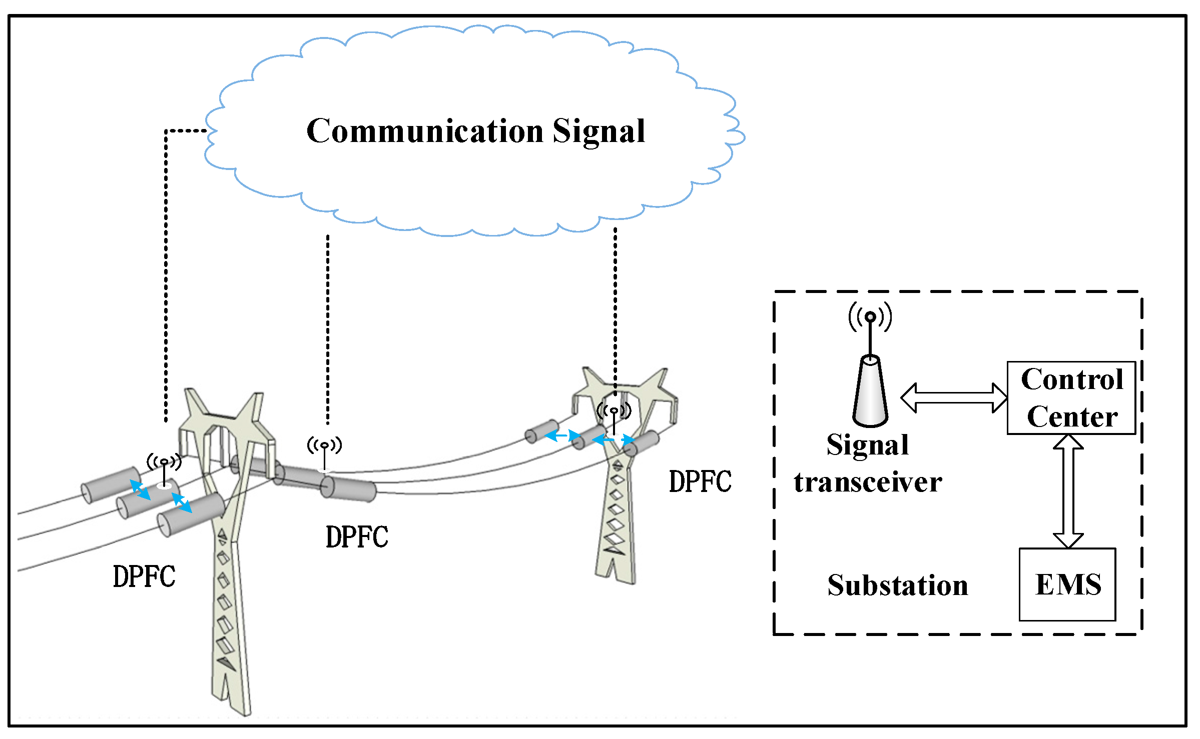
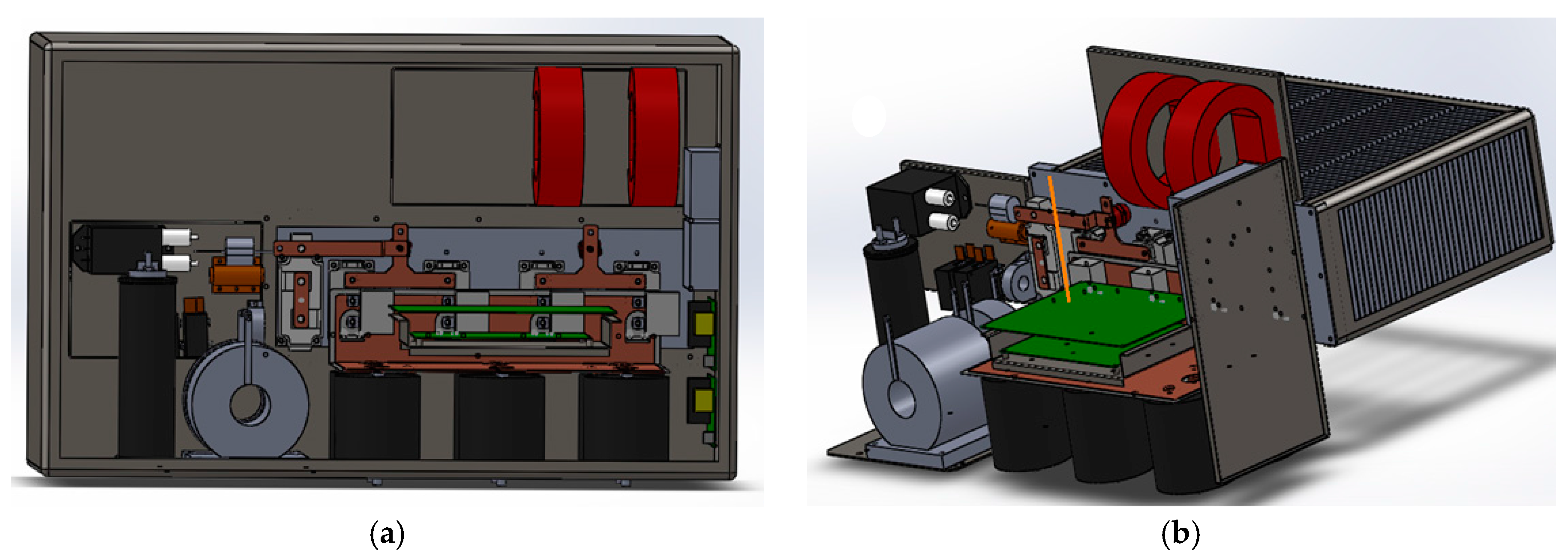
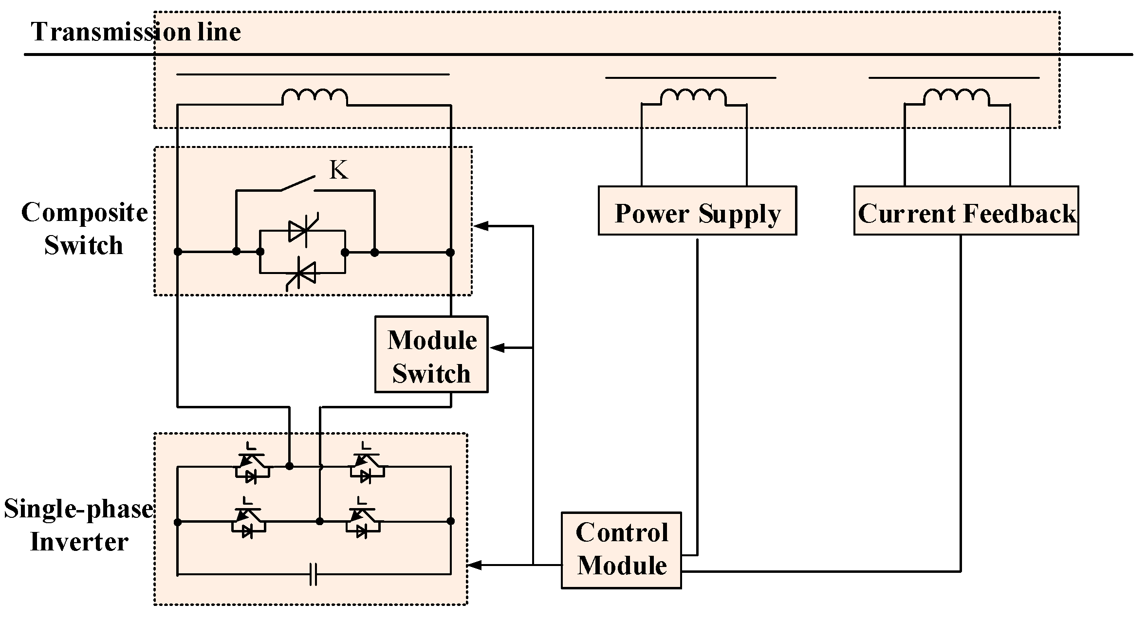
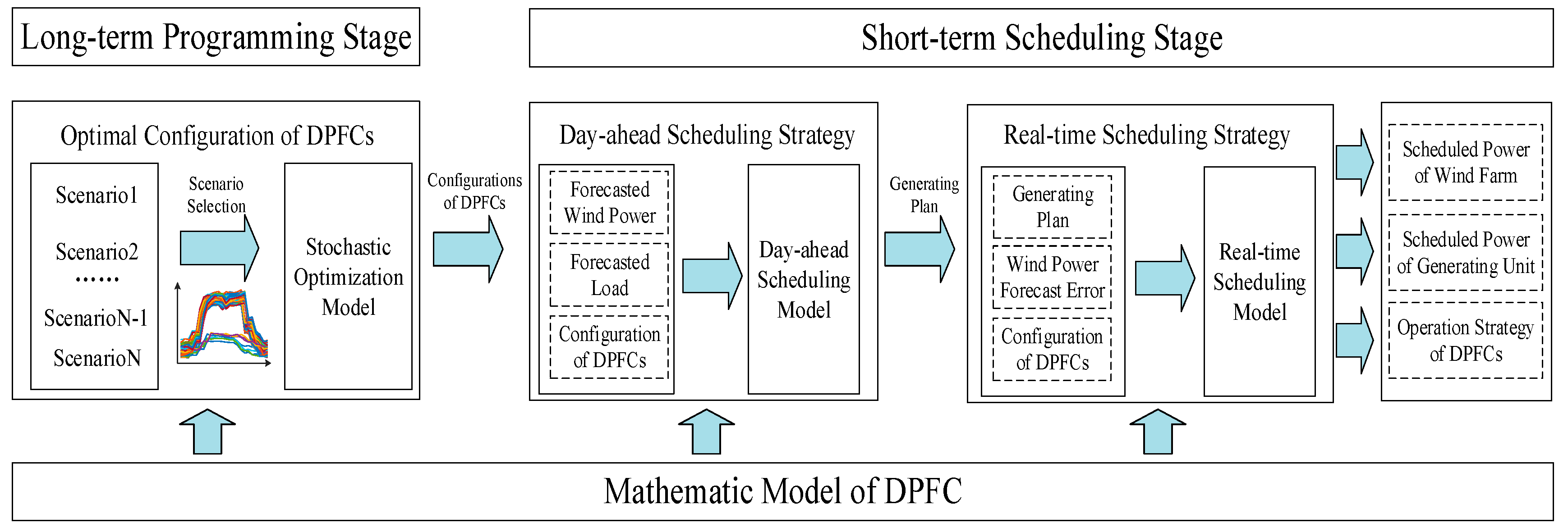
2. Structure and Mathematic Model of DPFC

2.1. Structure of DPFC

As shown in Figure 1, a DPFC can be directly installed on the conductor, which allows it to overcome many drawbacks of existing lumped FACTS technologies. The remarkable benefits are as follows: (i) ability to match the investment with the actual increase of load demand; (ii) ability to adjust the locations according to the change of load and wind power; (iii) flexible installation does not require an additional footprint; (iv) avoidance of high voltage insulation, which reduces manufacturing costs.
Figure 2 shows an electro-mechanical concept diagram for a DPFC and Figure 3 shows the schematic representation of the DPFC containing a single turn transformer (STT), a low-power single-phase inverter, a communication module and a composite switch. The inverter injects a desired quadrature voltage into the transmission line once it is activated. DPFC installed on lines is controlled by the control center deployed in the substation and system commands are received from the energy management system (EMS). Thus, the operation settings of DPFCs are adjusted rapidly by the control center as the change of load or power supply. The inverter and communication module are self-powered by induction from the conductor. The composite switch contains a normally closed electromechanical switch and a thyristor switch. The electromechanical switch is utilized to bypass the DPFC if the transmission line current is relatively small. With this switch closed, only a minimal level of reactance corresponding to the STT leakage reactance is inserted into the line, which has an extremely low impact on the power flow. The thyristor switch is used to ensure that the DPFC is bypassed quickly if a fault is detected by the current feedback signal.
By converting the module switch and the composite switch according to system commands, a DPFC can operate in the following two modes: (i) series reactor mode and (ii) reactive voltage injection mode. If the line current is slightly larger than the maximum acceptable level which is determined by transmission system operators considering the thermal constraints, transient or static stability limits, a DPFC is controlled to operate in series reactance mode and the STT magnetizing inductance is inserted into the transmission line to reduce the power flow. The injected inductance can be tuned to the desired value by installing a large number of DPFCs. It can be seen that the series reactor mode has minimal complexity. However, the current feedback signal is necessary to activate the single-phase inverter when line current is already close to its thermal limit. Thus, a DPFC can inject a quadrature voltage into the transmission line to simulate a positive or negative reactance in that mode, which can dynamically control the real power flow. Therefore, its function is similar to the static synchronous series compensator (SSSC).
According to the principle of power flow control utilizing DPFCs, power flow controllability of a DPFC in the second mode is superior to one in the first mode. Therefore, the mathematic model of DPFC is formulated based on the reactive voltage injection mode.

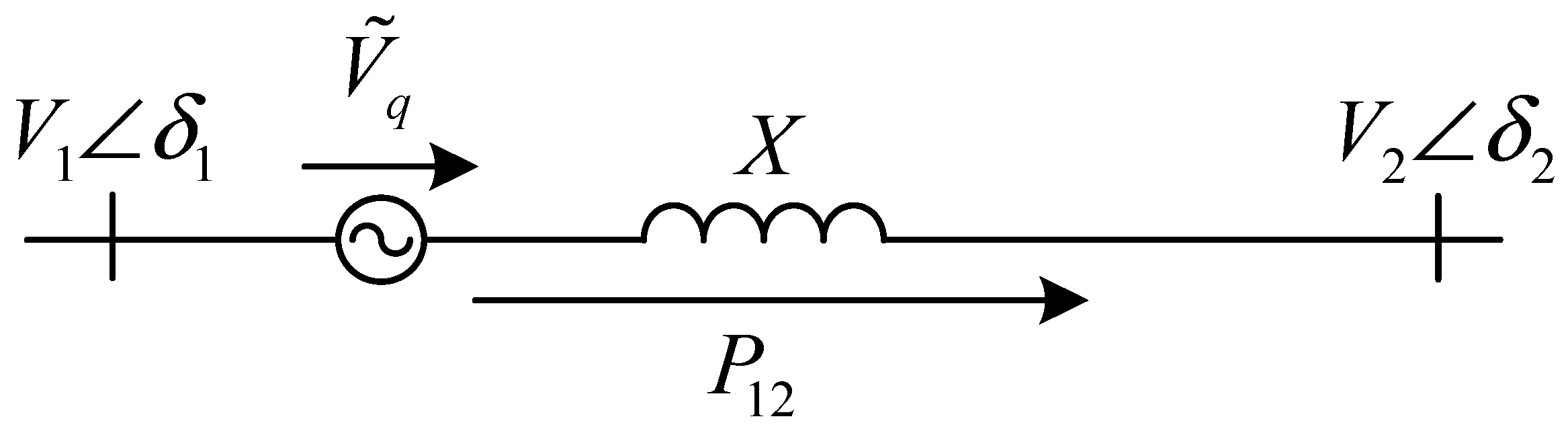
2.2. Linear Mathematic Model of DPFC

Figure 4 presents the circuit model of a DPFC deployed on a transmission line without considering the line resistance. V1 and V2 are the voltage amplitudes of sending and receiving end buses. X represents the reactance of the transmission line. Vq represents the voltage injected by a DPFC. Therefore, the relationship of line current and the voltage injected by a DPFC can be described as follow:
V ˜ q = ± j | V q | I ˜ | I ˜ | ,
where the unit vector in the direction of line current vector is represented by I ˜ | I ˜ | .
The series injected voltage clearly has an impact on controlling line power flow. The real power flow P12 along a transmission line deployed with a DPFC can be described as (2) by assumption that the voltage amplitudes of buses 1 and 2 are equal to V and the angle difference is equal to δ .
P 12 = V 2 X sin ( δ ) ± V | V q | X cos ( δ / 2 ) .
Since a DPFC is utilized to control real power flow and installed in the high voltage level transmission network, the DC power flow model is used in this paper for the mathematic formulation of the DPFC. In the DC model, the voltage amplitudes of all buses are assumed equal to 1 p.u., and voltage phase angle differences are assumed to be extremely small. Therefore, the active power flow given in (2) can be simplified as:
P 12 = δ X ± | V q | X .
Utilizing the linearization model of DPFC in (3), the injected voltage of DPFC can be embedded in the optimization model as a continuous control variable and solved by a linear programming solver.

3. Problem Formulation

The uncertainty of wind power brings new challenge to the scheduling of wind power. The accuracy of wind power forecast is closely related to the time scale. The shorter forecast horizons achieve the higher accuracy in wind power forecast error. Therefore, in order to reduce the wind power spillage, this paper designs a stochastic programming model of DPFCs considering many scenarios and establishes a sequential optimization scheduling model with DPFCs for maximum utilization of wind power so that system dispatchers can make reasonable scheduling planning of wind farms and generating units.
Figure 5 shows the two-stage scheduling framework containing multi-time scale for power systems integrating wind power considering DPFCs. Firstly, considering the uncertainty of the scenarios in the planning period, the stochastic programming method is used to determine the comprehensive configuration scheme of DPFCs in the first stage. In the second stage, two sequential scheduling models are considered. Combined with the given configuration scheme of DPFCs, the day-ahead scheduling model with the objective to minimize generation costs according to the forecast value of wind power and demand in day-ahead market. Afterward, the real-time scheduling model is used to eliminate the deviation of power generation plans caused by wind power forecast error. About 1 h prior to power delivery, the real-time scheduling is clear and final values for power consumptions and operation setting points are assigned to each generating unit and DPFC, respectively.

3.1. Stochastic Programming Model of DPFC

3.1.1. Objective Function

The main objective in long-term optimal configuration stage of DPFCs is to minimize wind power spillage and several scenarios are utilized to simulate the uncertainty of demand and wind power. The probability of each scenario represents the frequency of occurrence during the programming period of DPFCs.
Therefore, the objective of DPFCs’ stochastic programming model considering the scenarios is formulated as follows:
min s ρ s [ t ( w C w P w t s + g C g P g t s ) ] ,
where ρ s is the probability of scenario s; P w t s and P g t s are real power outputs for wind farm w and generating unit g at period t in scenario s, respectively; Cw and Cg are operation costs of wind farm w and unit g, respectively.

3.1.2. Constraints

(1)
Power Balance Constraints for Each Bus:
k δ + ( n ) L k t s k δ ( n ) L k t s + g g ( n ) P g t s + w w ( n ) P w t s = D n t s ,
where L k t s is real power flow through line k at period t in scenario s; D n t s is the active power consumption by load d at period t; δ + ( n ) and δ ( n ) are set of lines specified as to and from bus n, respectively.
(2)
Line Power Flows Equations:
L k t s B k ( θ m t s θ n t s ) B k V q k t s = 0 ,
where θ n t s is voltage angle of bus n at period t in scenario s; V q k t s is injected voltage of DPFC in line k at period t in scenario s; Bk is susceptibility of line k.
(3)
Generation Units Constraints:
0 P w t s P w t s f ,
P g t s P g min ,
P g t s + R S V g t s P g max ,
| P g t s P g t 1 s | R g H ,
where P w t s f is forecast value of wind farm w at period t in scenario s; P g max and P g min are upper and lower limits on the active power of generating unit g; R S V g t s is scheduled spinning reserve for unit g at period t in scenario s; R g H is maximum hourly ramp rate of unit g.
(4)
Reserve Constraints:
R S V t s r e q g R S V g t s ,
R S V g t s η R g H ,
where R S V t r e q is the required level of spinning reserve at period t; η is ratio of hourly ramp rate and short-time ramp rate.
(5)
Network Security Constraints:
| L k t s | L k lim ,
π θ n t s π ,
where L k lim is the thermal limit of transmission line k.
(6)
DPFC’s Constraints,
(a)
installation number constraints of DPFC:
N k min × u k N k N k max × u k ,
3 × k Ω l N k N T ,
where Nk is the number of DPFC installed on line k; uk is a binary parameter that specifies whether it is feasible to install DPFCs on line k; NT is the maximum total number of DPFCs available to be installed in the system; N k max and N k min are the maximum and minimum number of DPFCs installed on the line k. Since DPFCs are directly installed on the transmission lines, N k max is affected by the length of the line, the bearing capacity of the tower and the weight of the DPFC.
(b)
operation constraints of DPFC:
N k V q k min V q k t s N k V q k max ,
V q k max and V q k min are upper and lower limits on voltage injected by DPFC installed on the line k which can be calculated using the following equations:
V q k . max = S D P F C / I k . max ,
V q k . min = S D P F C / I k . max ,
where SDPFC is the capacity of each DPFC; Ik.max is the thermal limit of line k.
This stochastic programming method determines the optimal configuration of DPFC that appropriates for any plausible scenarios. Therefore, the output variables delivered to the second stage are Nk.

3.2. Day-Ahead Scheduling Model

3.2.1. Objective Function

According to the forecast data of demand and wind power, day-ahead scheduling model is proposed with the objective to minimize the total operation costs in the day-ahead market. Therefore, the objective is formulated as:
min T ( w C w P w . k . t + g C g P g . k . t ) ,

3.2.2. Constraints

Constraints in day-ahead scheduling model also consist of power equations, generation unit constraints, reserve constraints and security constraints which are formulated as follows:
k δ + ( n ) L k t k δ ( n ) L k t + g g ( n ) P g t + w w ( n ) P w t = D n t ,
L k t B k ( θ m t θ n t ) B k V q k t = 0 ,
0 P w t P w t f ,
P g t P g min ,
P g t + R S V g t P g max ,
| P g t P g t 1 | R g H ,
R S V t s r e q g R S V g t ,
R S V g t η R g H .
As mentioned before, the configuration of DPFCs containing location and number has been determined, hence DPFCs can only alter their injected voltages in this stage. Therefore, the constraint of DPFCs is formulated as follows:
N k f i x V q k min V q k t N k f i x V q k max ,
where N k f i x represents installed number of DPFCs on line k determined before.
The day-ahead scheduling model identifies variables P g t which are delivered to the next stage as constraints.

3.3. Real-Time Scheduling Model

In the real-time scheduling stage, final outputs of power generations would adjust for delivery of reserve needed for particular wind power forecast error. Therefore, considering the consecutiveness of multi-time scales, outputs of power generations should be modified based on the results given in day-ahead market solution. References [24,25] indicate that wind power forecast error is close to Laplace distribution whose probability density function is:
Δ P w t f = 1 2 λ exp ( λ | P w t f | ) ,
where Δ P w t f is wind power forecast error at period t. The parameter λ fitting the Laplace distribution of wind power forecast error is 38.22 in [24]. Hence, the actual schedulable power of wind farm k is expressed by Δ P w t f + P w t f .

3.3.1. Objective Function

Real-time scheduling model is proposed with the objective to minimize the total operation costs hourly. Therefore, the objective is formulated as:
min ( w C w P w k t + g C g P g k t ) .

3.3.2. Constraints

Constraints in real-time scheduling model are presented as follow:
k δ + ( n ) L k t k δ ( n ) L k t + g g ( n ) P g t + w w ( n ) P w t + w w ( n ) Δ P w t = D n t ,
L k t B k ( θ m t θ n t ) B k V q k t = 0 ,
0 P w t P w t f + Δ P w t f ,
P g min P g t P g max ,
R g H P g t P g t R g H ,
| L k t | L k lim ,
π θ n t π ,
N k f i x V q k min V q k t N k f i x V q k max ,
where P g t is scheduled power of generating unit g at period t in day-ahead market. Constraints (32) and (34) limit the power for each bus and outputs of wind farm considering the wind power forecast error, respectively. Constraint (36) limits the rescheduled outputs of generating units.
Final optimization results pertaining to the real-time scheduling stage are:
(1)
the final scheduled power of generating units;
(2)
the final scheduled power of wind farms;
(3)
the real-time operation control strategy of DPFCs.

4. Simulation Results
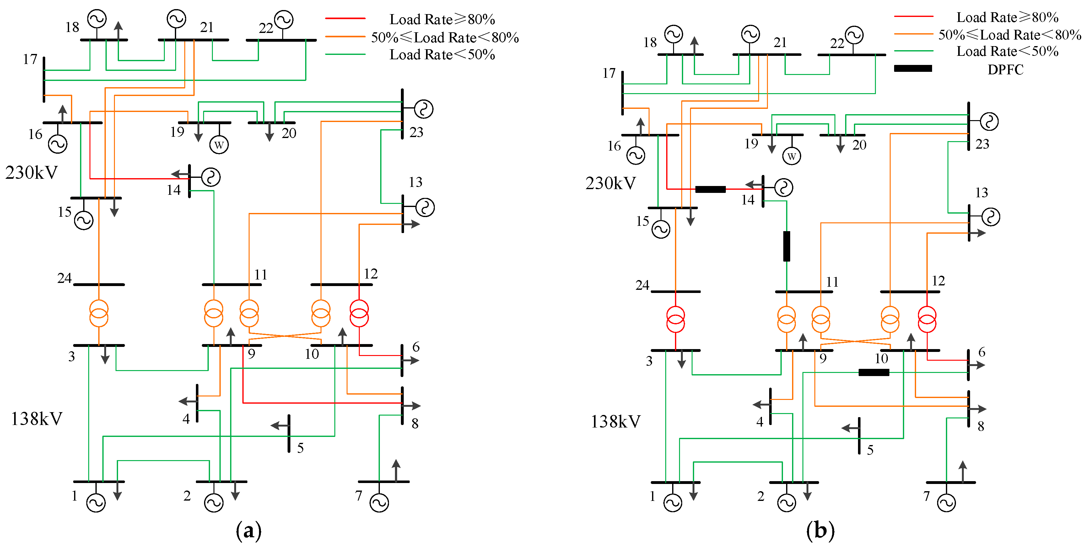
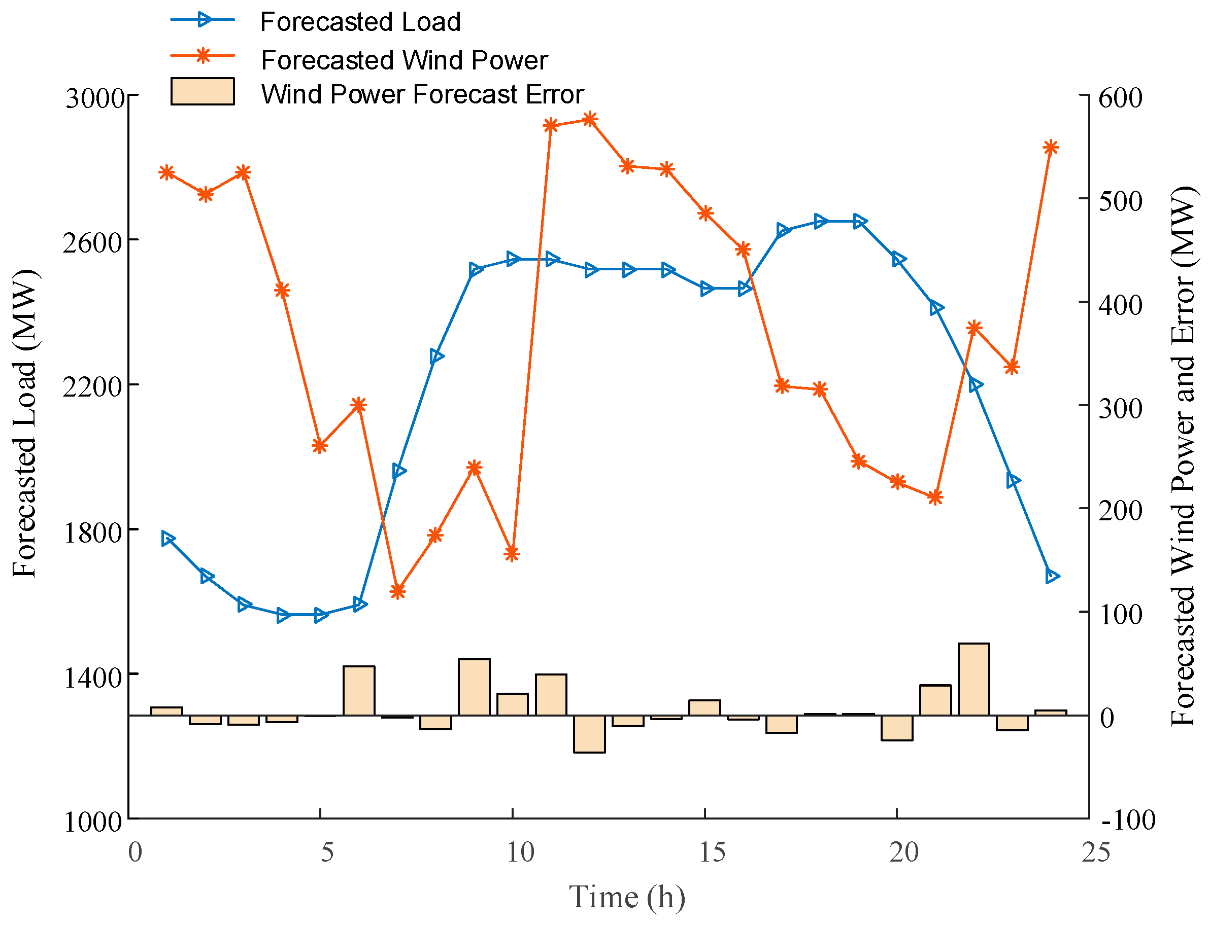
4.1. Data

This section presents numerical results for case study based on the IEEE-RTS79 system and the complete data of this test system can be obtained from [26]. To analyze the effect of DPFCs on the wind power spillage and verify the correctness and validity of the proposed method, a wind farm is considered and located at bus 19. The generation capacity of wind power is 800 MWA and its power factor is assumed to be equal to one. System daily load data can be obtained from [27]. For the maximum utilization of wind power, the values for operation costs of wind farm in objective function (4), (20) and (31) are assumed equal to 0. In order to better illustrate the effects of the proposed method, the transmission limits of all lines in the system are reduced by 50%. Besides, since the capacity of a DPFC is set to 70 kVA, the injected voltages of DPFCs installed on different transmission lines are shown in Table 1.
The maximum and minimum numbers of DPFCs allowed to be installed on a conductor of a transmission line must be specified. Since DPFCs can only be attached to the lines closely connected to the strain tower and there is approximately one strain tower per mile of a transmission line, the maximum number of DPFC installed on a transmission line is assumed equal to one per mile per conductor by considering the weight of DPFCs and the distribution of strain towers. The minimum number of DPFCs on each line is assumed equal to zero.
The following cases are considered for the verification purpose:
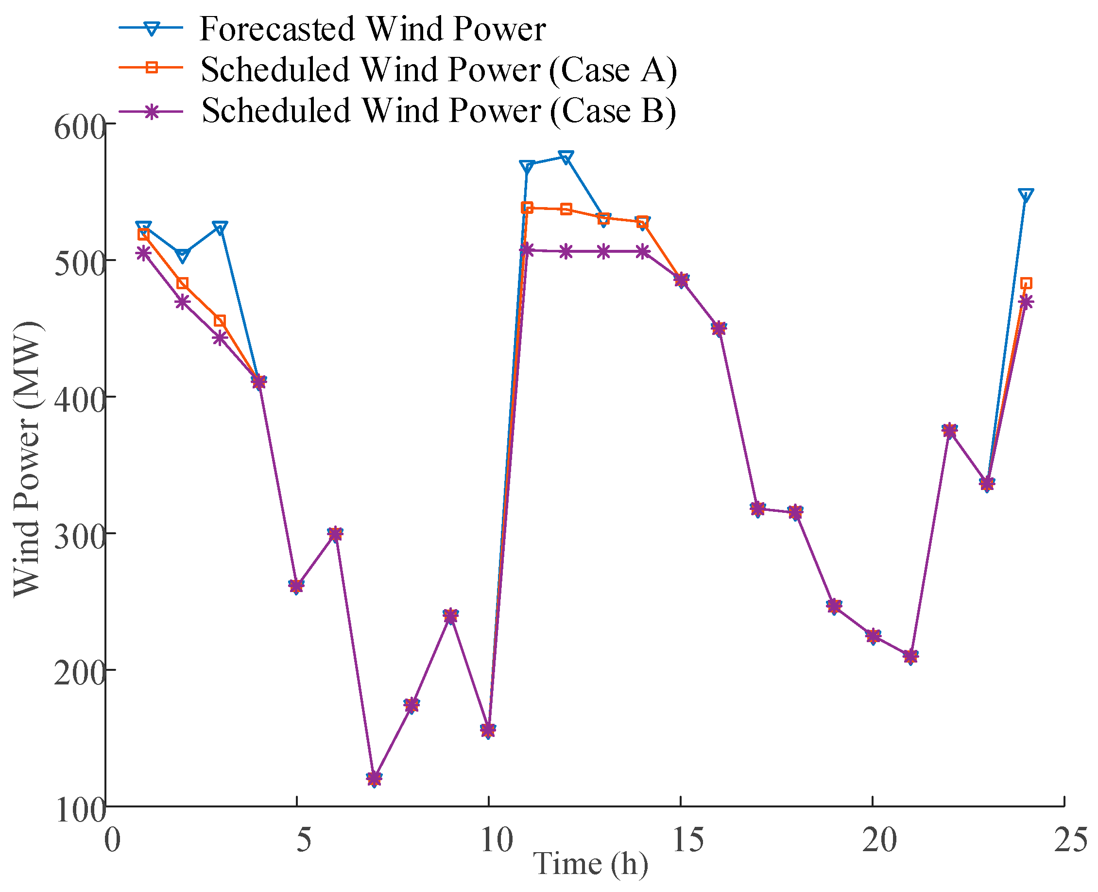
  • Case A: 150 DPFCs are installed by the proposed method.
  • Case B: No DPFCs in the system.
These cases are copped with the optimization model proposed previously and the results are presented in the following.

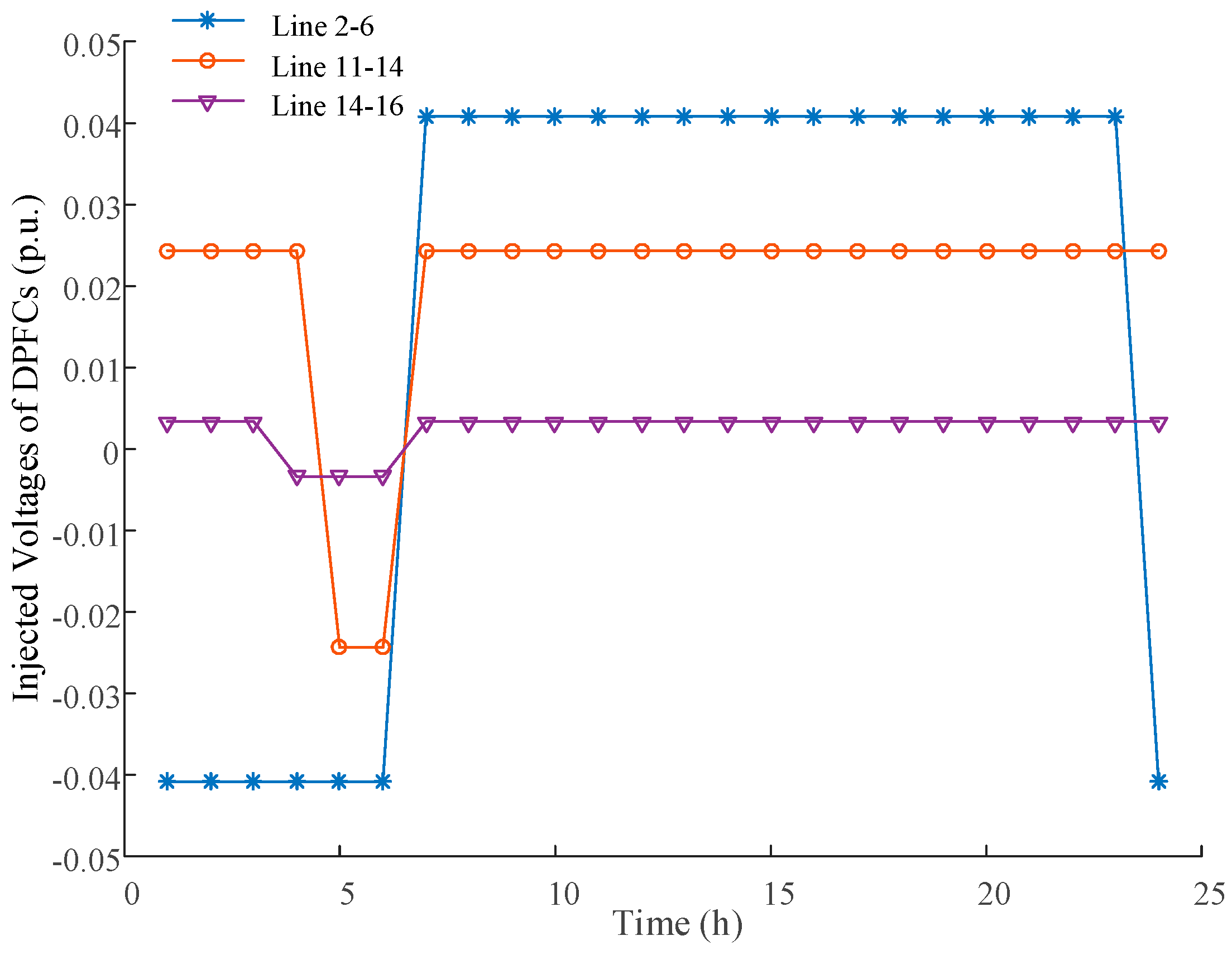
4.2. Optimal Configuration of DPFC

As depicted in Section 2.1, the locations of DPFCs can be adjusted according to the change of load and wind power. In fact, the locations of DPFCs are changed only once a quarter considering the transportation cost. Therefore, transmission system operators (TSOs) should make “configuration decisions” appropriate for any plausible load and wind power forecasted in the next quarter through a set of scenarios. For the sake of simplicity, TSOs usually select several scenarios occurring frequently as typical scenarios representing the operation state of system. Hence the scenarios are determined by TSOs based on historical operational data and forecasts of economy and meteorology. However, the computation time may become intractable if too much scenarios are considered. In order to simplify the calculation, four typical scenarios are utilized to determine the optimal configuration of DPFCs in this paper. The probability of each scenario may be distinguishing in different power grids. Without losing the generality, the duration of each selected scenario is assumed to be identical and the probabilities of these scenarios are equal to 0.25.
Figure 6 shows the optimal power flows in IEEE-RTS79 system. The expected average load rates of lines are calculated based on (40):
L k R = s t ρ s L k t s L k lim .
The average load rates of lines 14–16 and 16–19 are 96.31% and 56.35%, respectively. The scheduling periods that load rates of these lines exceed 80% are 23 and 8, respectively. Therefore, the insufficient capacity of these two lines has significantly affected the wind power consumption. Table 2 shows the specific configuration of DPFCs. From Table 2 and Figure 6 it can be seen that 99 DPFCs are installed on lines 14–16 and 11–14. This configuration result is consistent with the engineering experience, i.e., FACTS devices are installed around the lines that are more heavily utilized.

4.3. Results of Day-Ahead Scheduling

Figure 7 shows the daily load curve and wind power forecast error calculated by (30). It can be seen from Figure 7 that there exists apparent difference between load and wind power.
Based on the configuration of DPFCs showed in Table 2, scheduled power of wind farm and generating units are optimized by day-ahead scheduling model. Figure 8 shows the comparison of scheduled wind power in two cases. The intermittent characteristics of wind power make the wind power spillage occurring in the period of peak load or sufficient wind energy, such as 1–4 h and 11–14 h. With the deployment of DPFCs, the wind power consumption has been increased from 96.85% to 98.97%.
From the optimized results of the power flow, it can be found that the load rates of double lines 19–20 are lower than 30% when the lines 16–19 and 14–16 are overload. Figure 9 shows the compassion of power flows in two cases. In case A with DPFCs deployed, the total expected value of wind power consumption is increased from 101.82 MW to 120.39 MW during the 1–4 h and 11–14 h that wind power spillage occurs. This implies that more transmission capacity has been utilized in reducing wind power spillage.

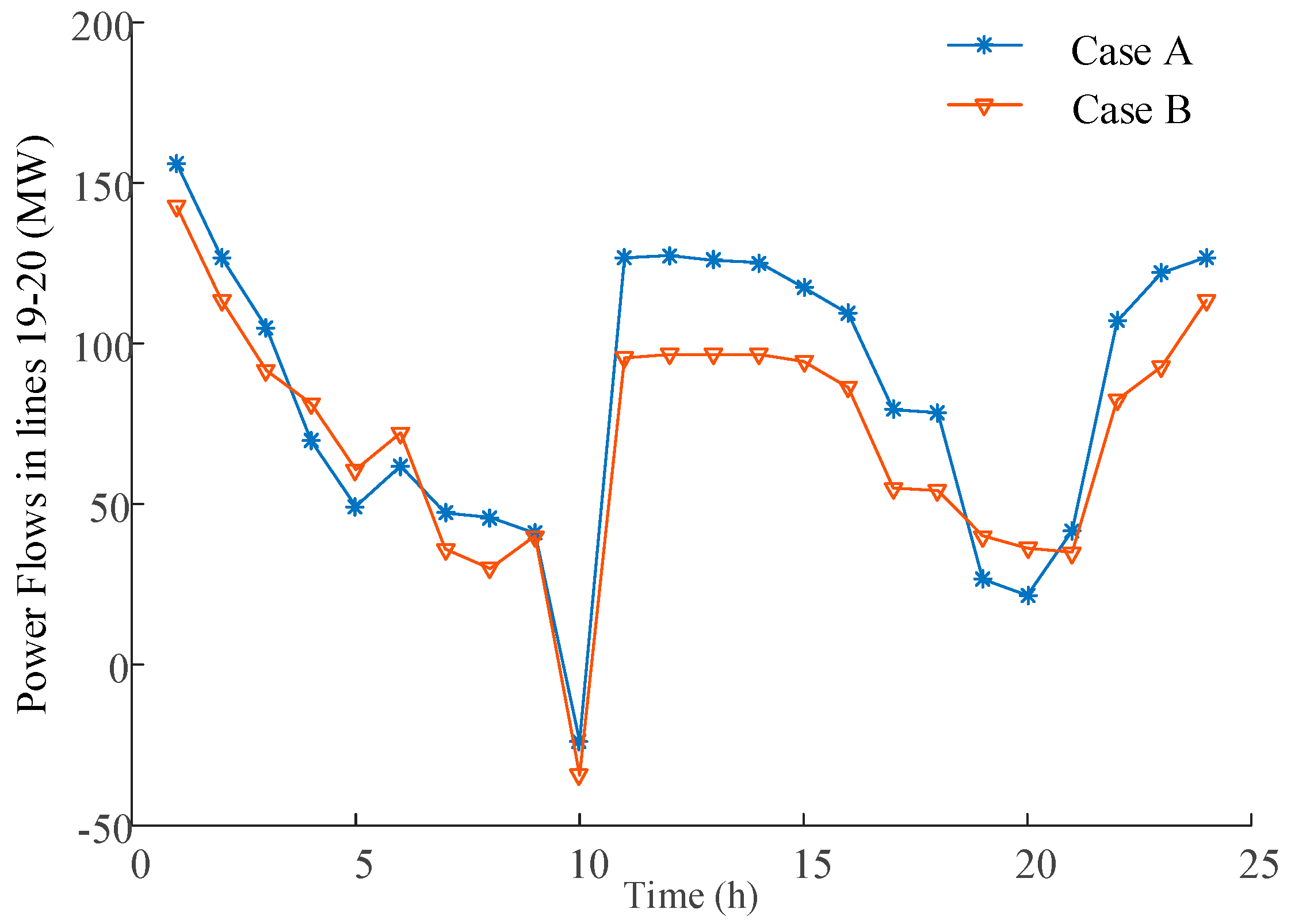
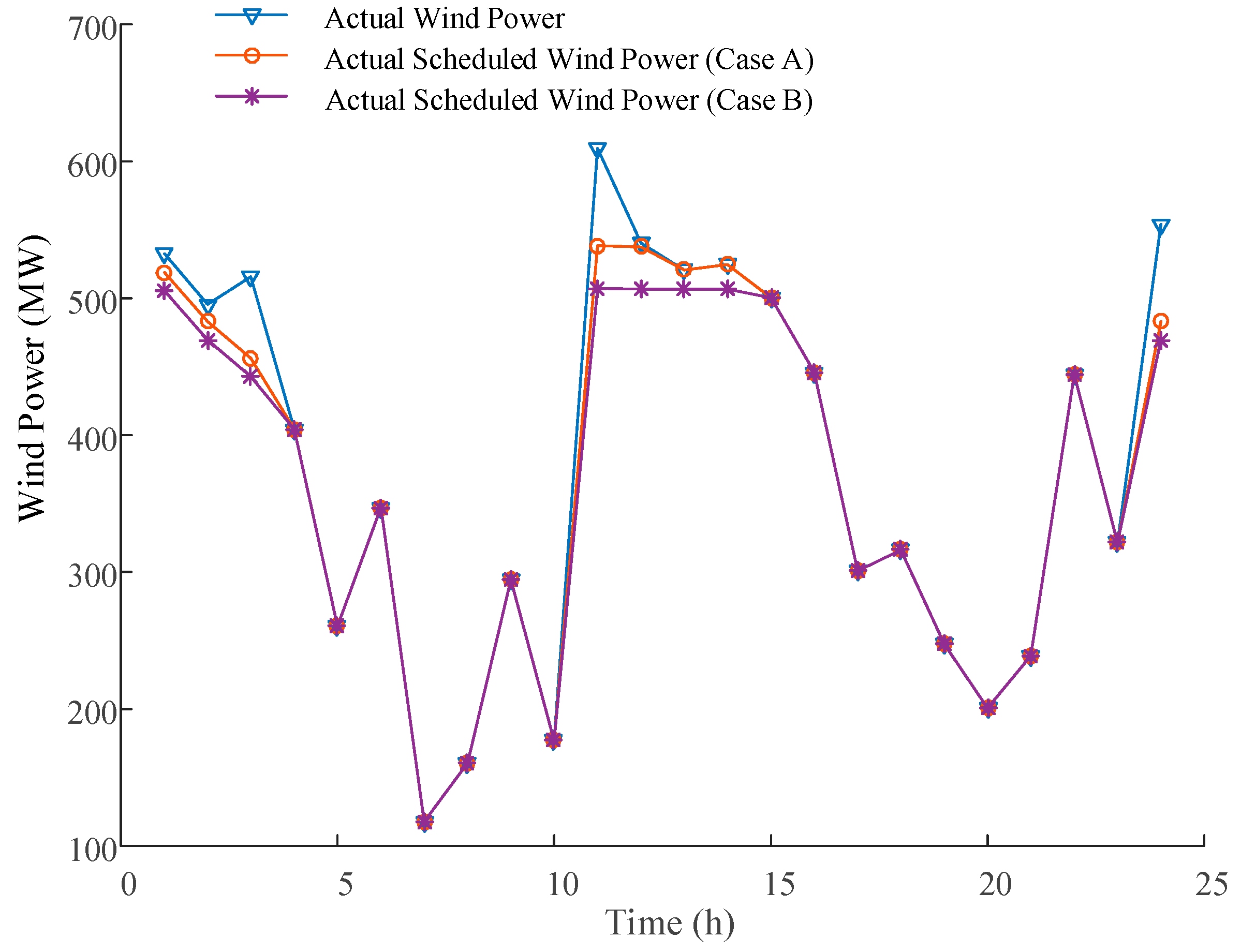
4.4. Results of Real-Time Scheduling

Figure 10 depicts the final scheduled power curve of wind farm. Accordingly, wind power spillage has occurred in two case and the amount of Case A is comparatively lower than Case B. Table 3 shows the final optimization results of cases. With the deployment of DPFCs to regulate power flows, the total consumption of wind power is increased from 8692.01 MWh to 8839.48 MWh and the final consumption rate is increased from 95.83% to 97.45%. Besides, compared with the day-ahead scheduling solutions, the wind power consumption is reduced slightly. This implies that wind power forecast error is not conducive to the consumption of wind power. Moreover, the periods that wind power occurred in have changed considering the forecast error. All the wind power has been scheduled in 18 h and total periods of wind power spillage are reduced from 8 to 5. Therefore, the total operation cost in Case A is lower than Case B.
If DPFCs are utilized to reduce wind power spillage, their optimal control strategy needs to be determined. Figure 11 illustrates the optimal injected voltage setting of DPFCs. Note that, the optimal setting of DPFC across periods often equal to their bounds for maximum capability in controlling power flows and injected voltage of DPFCs adjusts along with the change of wind power and loads. As shown in Figure 6, lines 16–19 and 19–20 constitute the transmission interface of wind power deployed in bus 19. During the periods that wind spillage occurs, DPFCs operating in capacitive compensation on lines 14–16 and 11–14 can effetely control the power flows within thermal limits which makes the power flows in line 19-20 increase if wind power is abundant. Therefore, the flexibility in power flow control can utilize the total transfer capacity of transmission interface which is conducive to the consumption of wind power.

5. Conclusions

This paper proposes a multi-time scale scheduling methodology with DPFCs in system with high penetration of wind power. The optimal configuration of DPFCs is determined considering several plausible scenarios in the long-term scale. In the short-term scheduling stage consists of day-ahead and real-time scale, economic scheduling plans containing control strategy of DPFCs and scheduled power of several energies are obtained while considering uncertainty of wind power and physical and operating limitations on DPFCs. The case studies for the IEEE-RTS79 system illustrate the effectiveness of the proposed method, which can offer more economically scheduling plan and maximum utilization of wind power when DPFCs are optimal deployed and controlled. The proposed methodology could be applied for other sorts of FACTS or D-FACTS devices to promote the utilization of wind energy in power systems.

Acknowledgments

This work is supported by the National Natural Science Foundation of China (Grant No. 51577030) and the Science and technology project of Jiangsu Electric Power Company Research Institute (Grant No. 8516000700).

Author Contributions

Yi Tang, Yuqian Liu and Jingbo Zhao contributed in developing the ideas of this research. Yi Tang, Yuqian Liu and Jia Ning performed this research. All the authors read and approved the final manuscript.

Conflicts of Interest

The authors declare no conflict of interest.

References

  1. Bruninx, K.; Delarue, E. A statistical description of the error on wind power forecasts for probabilistic reserve sizing. IEEE Trans. Sustain. Energy 2014, 5, 995–1002. [Google Scholar] [CrossRef]
  2. Li, P.; Guan, X.; Wu, J.; Zhou, X. Modeling dynamic spatial correlations of geographically distributed wind farms and constructing ellipsoidal uncertainty sets for optimization-based generation scheduling. IEEE Trans. Sustain. Energy 2015, 6, 1594–1605. [Google Scholar] [CrossRef]
  3. Lima, M.; Carvalho, P.; Carneiro, T.; Carneiro, T.; Leite, J.; Neto, L.; Rodrigues, G. Portfolio theory applied to solar and wind resources forecast. IET Renew. Power Gener. 2017, 11, 973–978. [Google Scholar] [CrossRef]
  4. Doostizadeh, M.; Aminifar, F.; Ghasemi, H.; Lesani, H. Energy and reserve scheduling under wind power uncertainty: An adjustable interval approach. IEEE Trans. Smart Grid 2016, 7, 2943–2952. [Google Scholar] [CrossRef]
  5. Zhang, N.; Kang, C.; Xia, Q.; Liang, J. Modeling conditional forecast error for wind power in generation scheduling. IEEE Trans. Power Syst. 2014, 29, 1316–1324. [Google Scholar] [CrossRef]
  6. Kargarian, A.; Hug, G.; Mohammadi, J. A multi-time scale co-optimization method for sizing of energy storage and fast-ramping generation. IEEE Trans. Sustain. Energy 2016, 7, 1351–1361. [Google Scholar] [CrossRef]
  7. Nikoobakht, A.; Mardaneh, M.; Aghaei, J.; Guerrero-Mestre, V.; Contreras, J. Flexible power system operation accommodating uncertain wind power generation using transmission topology control: An improved linearised AC SCUC model. IET Gener. Transm. Dis. 2017, 11, 142–153. [Google Scholar] [CrossRef]
  8. Liu, M.; Quilumba, F.; Lee, W. Dispatch scheduling for a wind farm with hybrid energy storage based on wind and LMP forecasting. IEEE Trans. Ind. Appl. 2015, 51, 1970–1977. [Google Scholar] [CrossRef]
  9. Bitaraf, H.; Rahman, S.; Pipattanasomporn, M. Sizing energy storage to mitigate wind power forecast error impacts by signal processing techniques. IEEE Trans. Sustain. Energy 2015, 6, 1457–1465. [Google Scholar] [CrossRef]
  10. Yuan, R.; Ye, J.; Lei, J.; Li, T. Integrated combined heat and power system dispatch considering electrical and thermal energy storage. Energies 2016, 9, 474. [Google Scholar] [CrossRef]
  11. Rong, S.; Li, Z.; Li, W. Investigation of the promotion of wind power consumption using the thermal-electric decoupling techniques. Energies 2015, 8, 8613–8629. [Google Scholar] [CrossRef]
  12. Xu, T.; Zhang, N. Coordinated operation of concentrated solar power and wind resources for the provision of energy and reserve services. IEEE Trans. Power Syst. 2017, 32, 1260–1271. [Google Scholar] [CrossRef]
  13. Hozouri, M.; Abbaspour, A.; Fotuhi-Firuzabad, M.; Moeini-Aghtaie, M. On the use of pumped storage for wind energy maximization in transmission-constrained power systems. IEEE Trans. Power Syst. 2015, 30, 1017–1025. [Google Scholar] [CrossRef]
  14. Pourmousavi, S.; Patrick, S.; Nehrir, M. Real-time demand response through aggregate electric water heaters for load shifting and balancing wind generation. IEEE Trans. Smart Grid 2014, 5, 769–778. [Google Scholar] [CrossRef]
  15. Ali, M.; Degefa, M.; Humayun, M.; Lehtonen, M. Increased utilization of wind generation by coordinating the demand response and real-time thermal rating. IEEE Trans. Power Syst. 2016, 31, 3737–3746. [Google Scholar] [CrossRef]
  16. Daraeepour, A.; Kazempour, S.; Patiño-Echeverri, D.; Conejo, A. Strategic demand-side response to wind power integration. IEEE Trans. Power Syst. 2015, 31, 3495–3505. [Google Scholar] [CrossRef]
  17. Yang, S.; Zeng, D.; Ding, H.; Yao, J.; Wang, K.; Li, Y. Multi-objective demand response model considering the probabilistic characteristic of price elastic load. Energies 2016, 9, 80. [Google Scholar] [CrossRef]
  18. Sahraei-Ardakani, M.; Blumsack, S. Transfer capability improvement through market-based operation of series FACTS devices. IEEE Trans. Power Syst. 2016, 31, 3702–3714. [Google Scholar] [CrossRef]
  19. Ullah, I.; Gawlik, W.; Palensky, P. Analysis of power network for line reactance variation to improve total transmission capacity. Energies 2016, 9, 936. [Google Scholar] [CrossRef]
  20. Divan, D.; Brumsickle, W.; Schneider, R.; Kranz, B.; Gascoigne, R.; Bradshaw, D. A distributed static series compensator system for realizing active power flow control on existing power lines. IEEE Trans. Power Deliv. 2006, 22, 642–649. [Google Scholar] [CrossRef]
  21. Nasri, A.; Conejo, A.J.; Kazempour, S.J.; Ghandhari, M. Minimizing wind power spillage using an OPF with FACTS devices. IEEE Trans. Power Syst. 2014, 29, 2150–2159. [Google Scholar] [CrossRef]
  22. Kapetanaki, A.; Levi, V.; Buhari, M.; Schachter, J. Maximization of wind energy utilization through corrective scheduling and FACTS deployment. IEEE Trans. Power Syst. 2017, 32, 4764–4773. [Google Scholar] [CrossRef]
  23. Elmitwally, A.; Eladl, A.; Morrow, J. Long-term economic model for allocation of FACTS devices in restructured power systems integrating wind generation. IET Gener. Transm. Dis. 2016, 10, 19–30. [Google Scholar] [CrossRef] [Green Version]
  24. Huo, Y.; Jiang, P.; Zhu, Y.; Feng, S.; Wu, X. Optimal Real-Time Scheduling of Wind Integrated Power System Presented with Storage and Wind Forecast Uncertainties. Energies 2015, 8, 1080–1100. [Google Scholar] [CrossRef]
  25. Su, H.; Gamal, A. Modeling and Analysis of the Role of Energy Storage for Renewable Integration: Power Balancing. IEEE Trans. Power Syst. 2013, 28, 4109–4117. [Google Scholar] [CrossRef]
  26. Subcommittee, P. IEEE reliability test system. IEEE Trans. Power Appl. Syst. 1979, 98, 2047–2054. [Google Scholar] [CrossRef]
  27. Conejo, A.; Carrion, M.; Morales, J. Appendix B 24-node system data. In Decision Making under Uncertainty in Electricity Markets; Springer Science + Business Media, LLC: New York, NY, USA, 2010; pp. 479–485. [Google Scholar]
Figure 1. Distributed power flow controller (DPFC) deployed on transmission line.
Energies 10 01804 g001
Figure 2. Electro-mechanical concept diagram of DPFC. (a) Front view of DPFC, and (b) Lateral view of DPFC.
Energies 10 01804 g002
Figure 3. Schematic representation of a DPFC.
Energies 10 01804 g003
Figure 4. Circuit model of a transmission line with DPFC.
Energies 10 01804 g004
Figure 5. Framework of multi-time scale scheduling strategy with DPFCs.
Energies 10 01804 g005
Figure 6. Power flows in IEEE-RTS79 system, (a) without DPFCs, and (b) with DPFCs.
Energies 10 01804 g006
Figure 7. Wind power curve and forecast error.
Energies 10 01804 g007
Figure 8. Scheduled power in day-ahead scheduling stage.
Energies 10 01804 g008
Figure 9. Power flows in line 19–20 in day-ahead scheduling stage.
Energies 10 01804 g009
Figure 10. Scheduled power in real-time scheduling stage.
Energies 10 01804 g010
Figure 11. Optimal control strategy of DPFCs in real-time scheduling stage.
Energies 10 01804 g011
Table 1. Injected voltage of DPFC on different voltage level transmission lines.
Maximum Injected VoltageMinimum Injected VoltageLine
VpuVPuVoltage (kV)Transmission Limit (MW)
191.222.4 × 10−3−191.22−2.4 × 10−313887.5
111.548.4 × 10−4−111.54−8.4 × 10−4230250
Table 2. Optimal configuration of DPFC.
LineNumber of DPFC
From BusTo BusLength/Mile
265051
11142987
14162712
Sum150
Table 3. Numerical results for cases considered.
CasesWind Power Consumption (MWh)Wind Power Consumption Percentage (%)Total Periods of Wind Power SpillageOperation Cost (Dollar)
Case A8839.4897.45526,774.72
Case B8692.0195.83827,114.59

