Implementation, Comparison and Application of an Average Simulation Model of a Wind Turbine Driven Doubly Fed Induction Generator


Abstract
:1. Introduction
2. Wind Turbine Driven DFIG Control
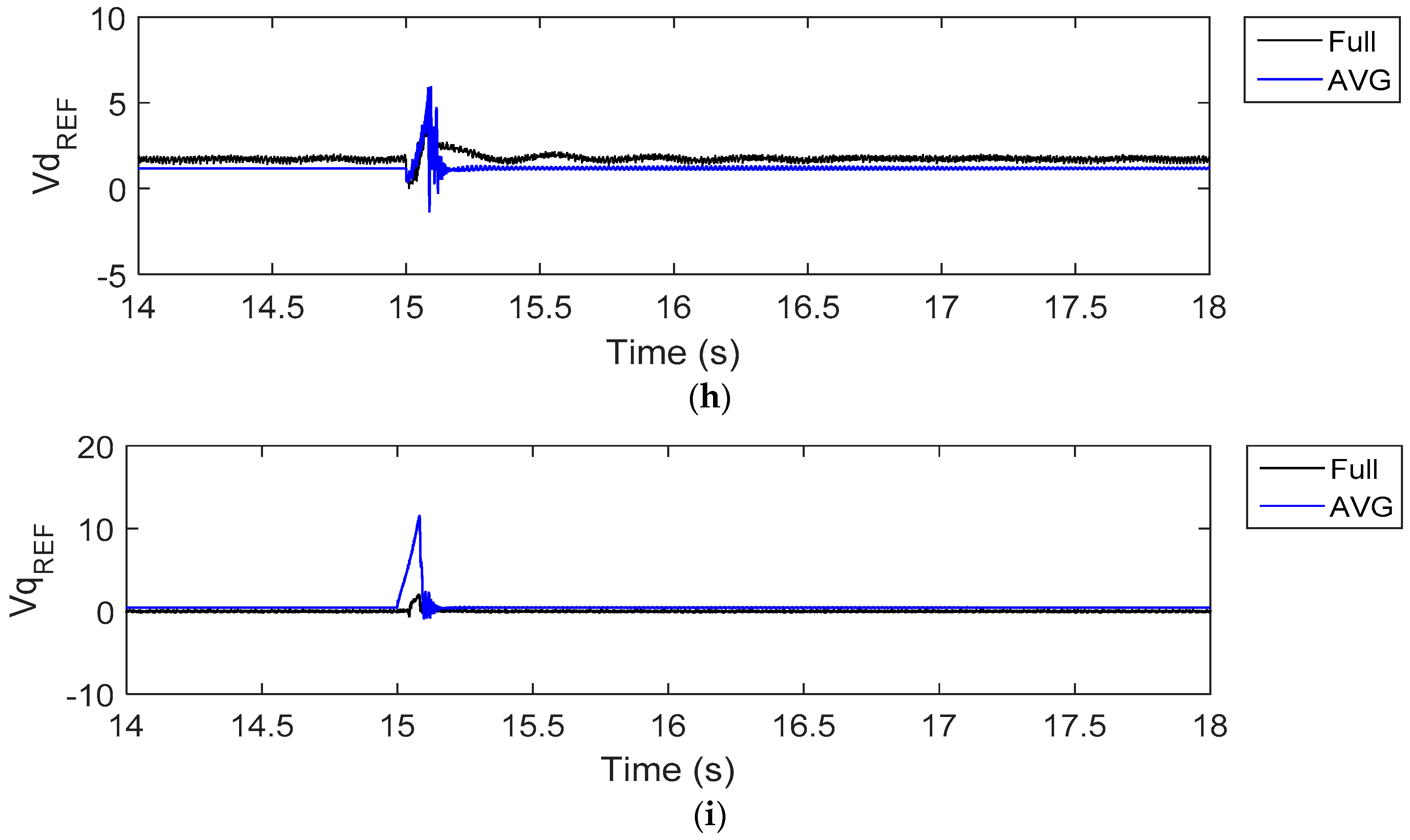
2.1. Converter Control in the Detailed Model of DFIG
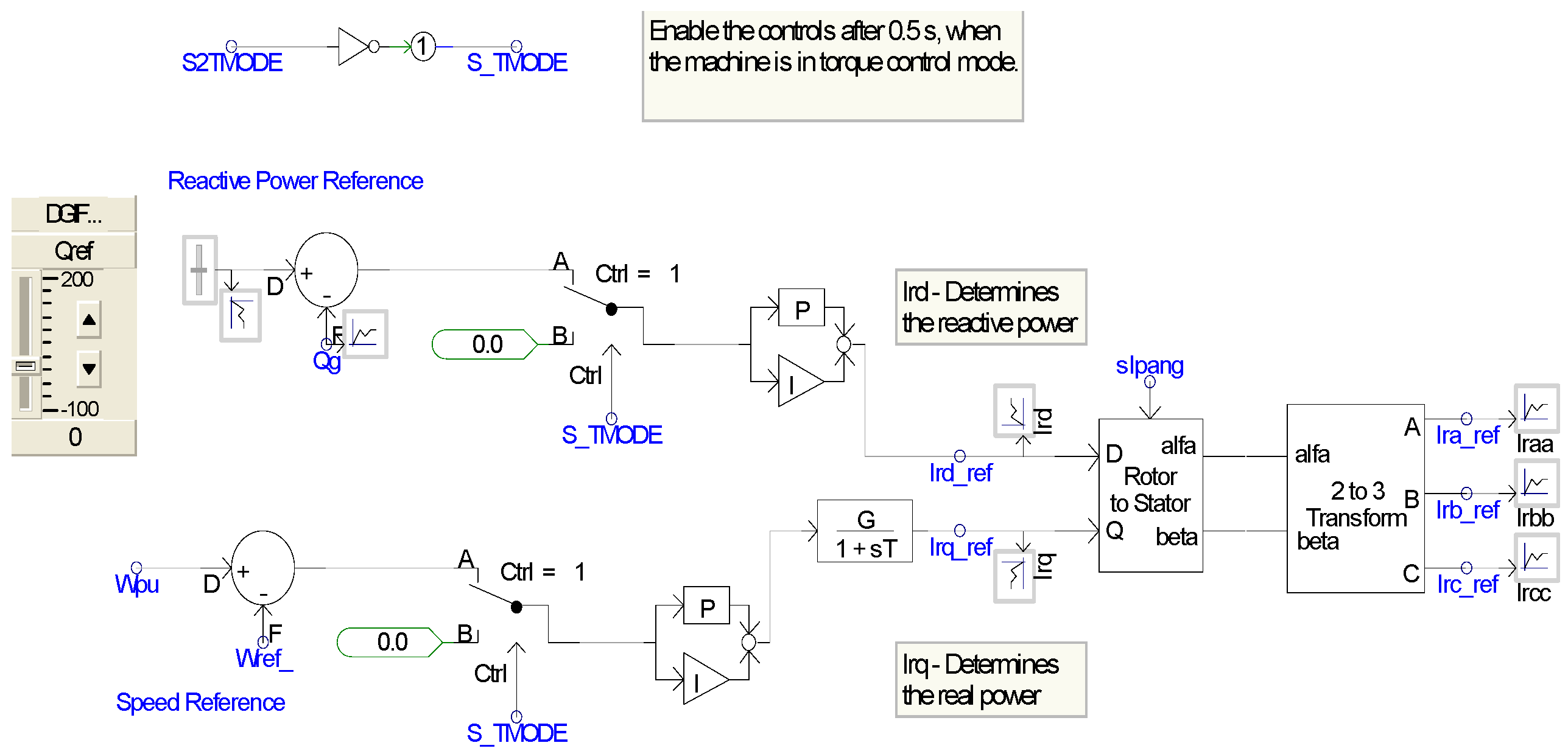
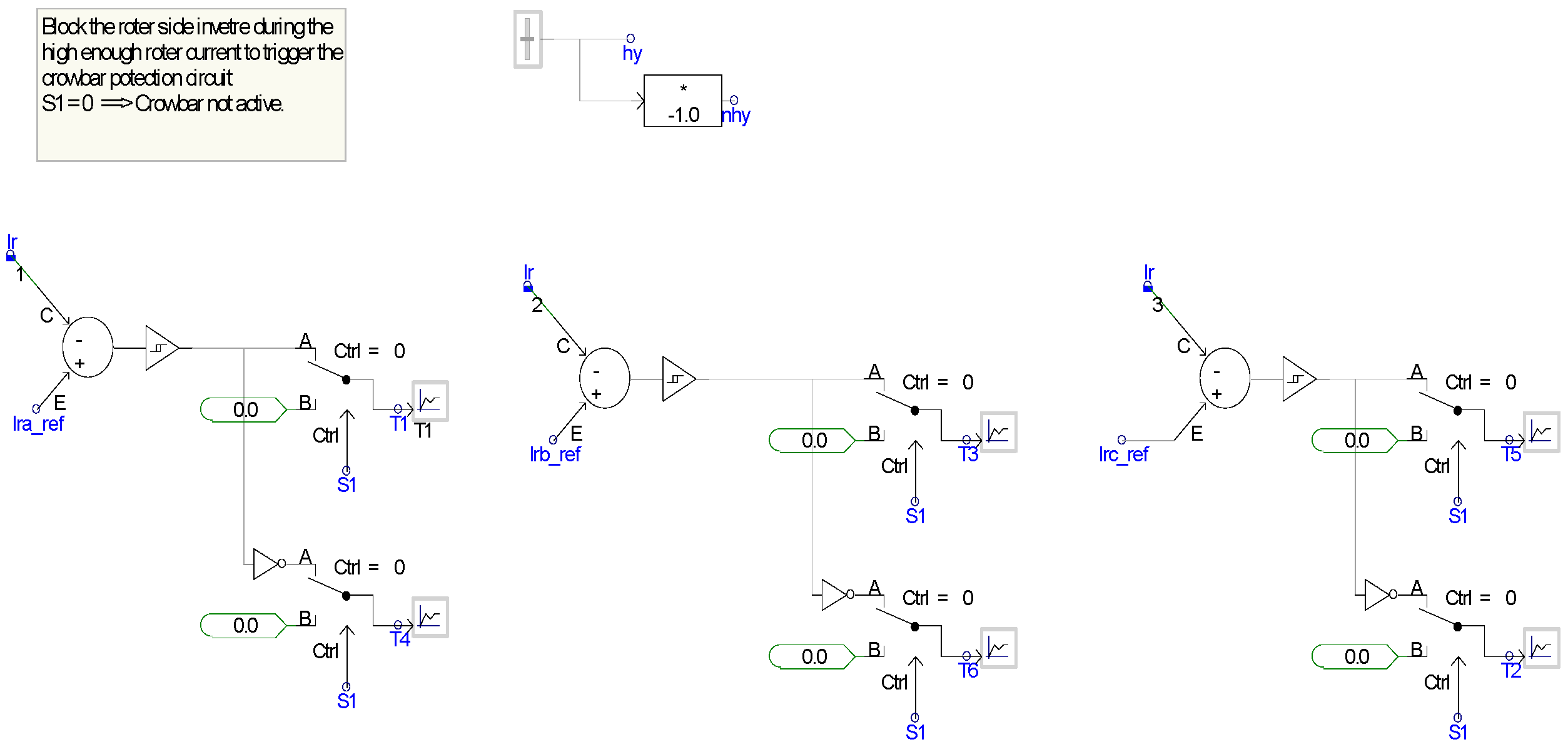
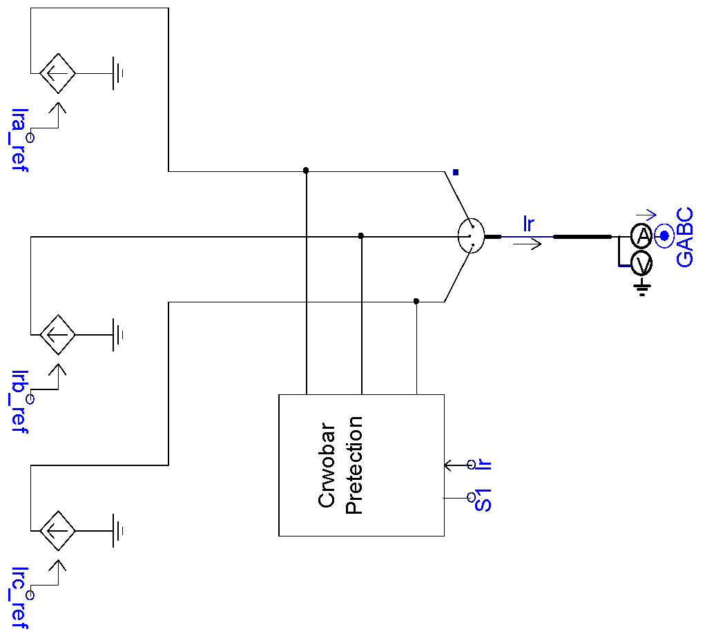
2.1.1. Rotor Side Converter Control
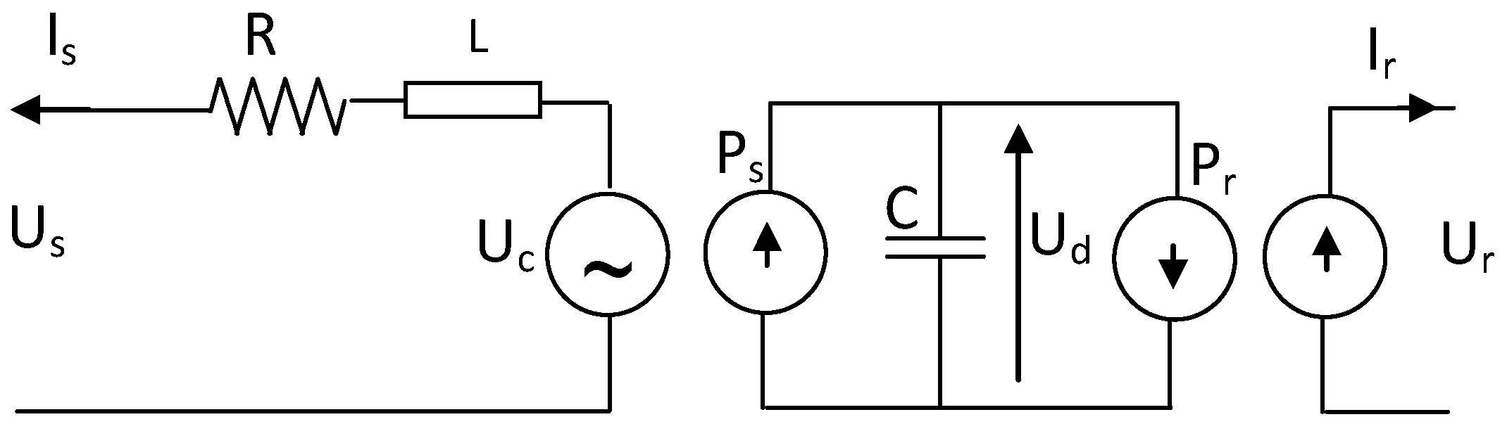
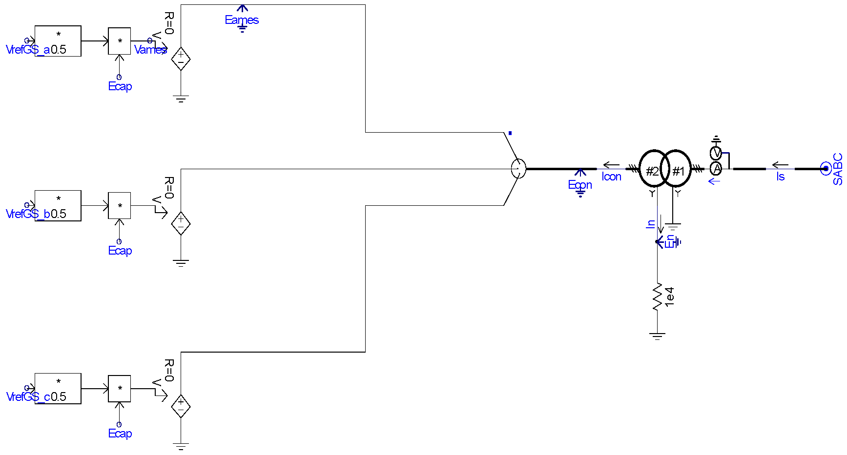
2.1.2. Grid Side Converter Control
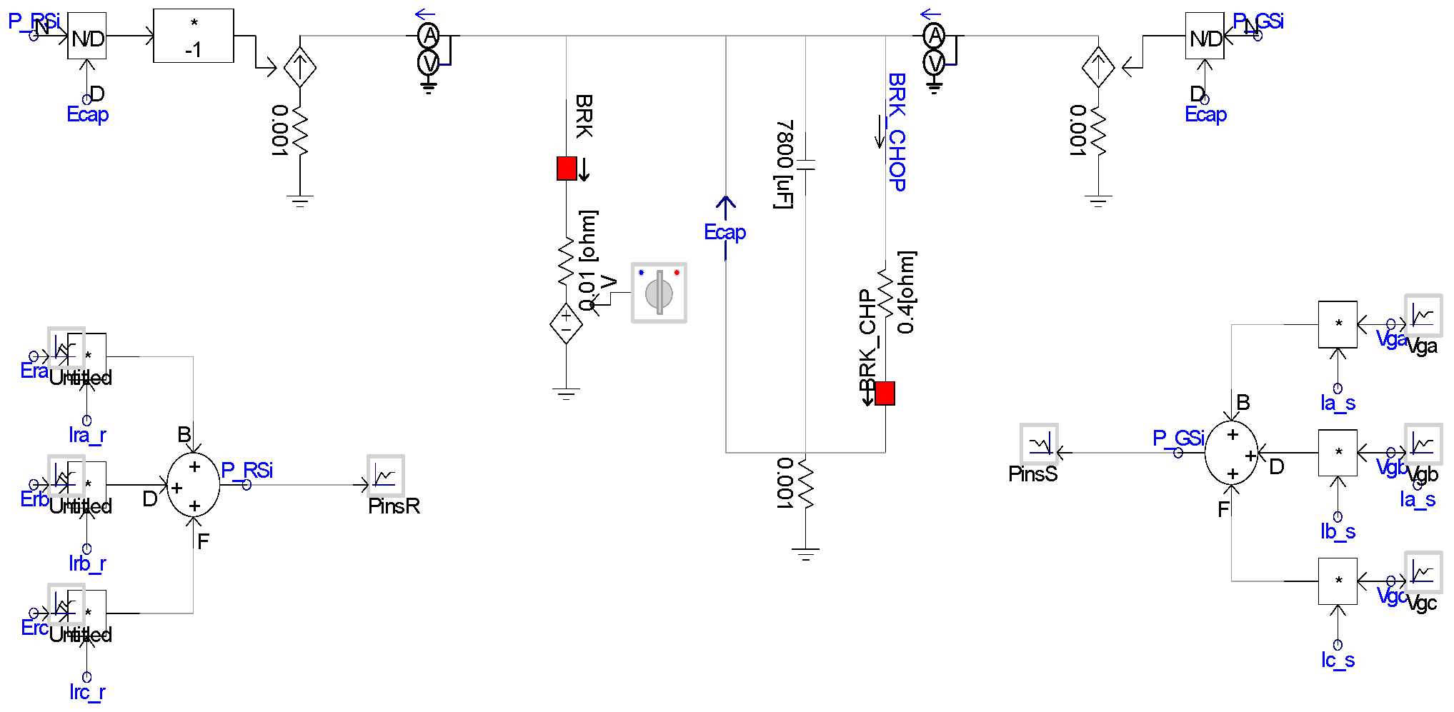
2.2. Average DFIG Model
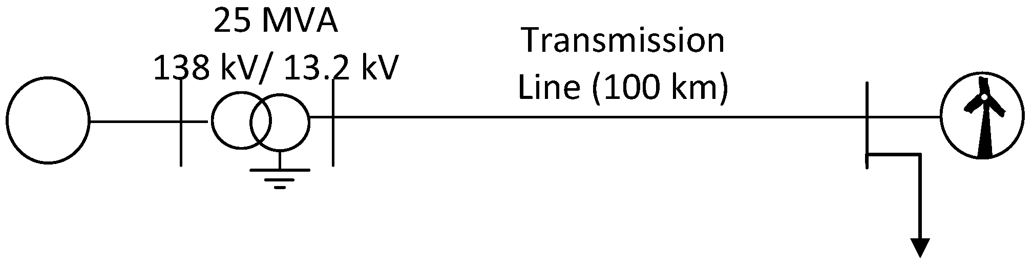
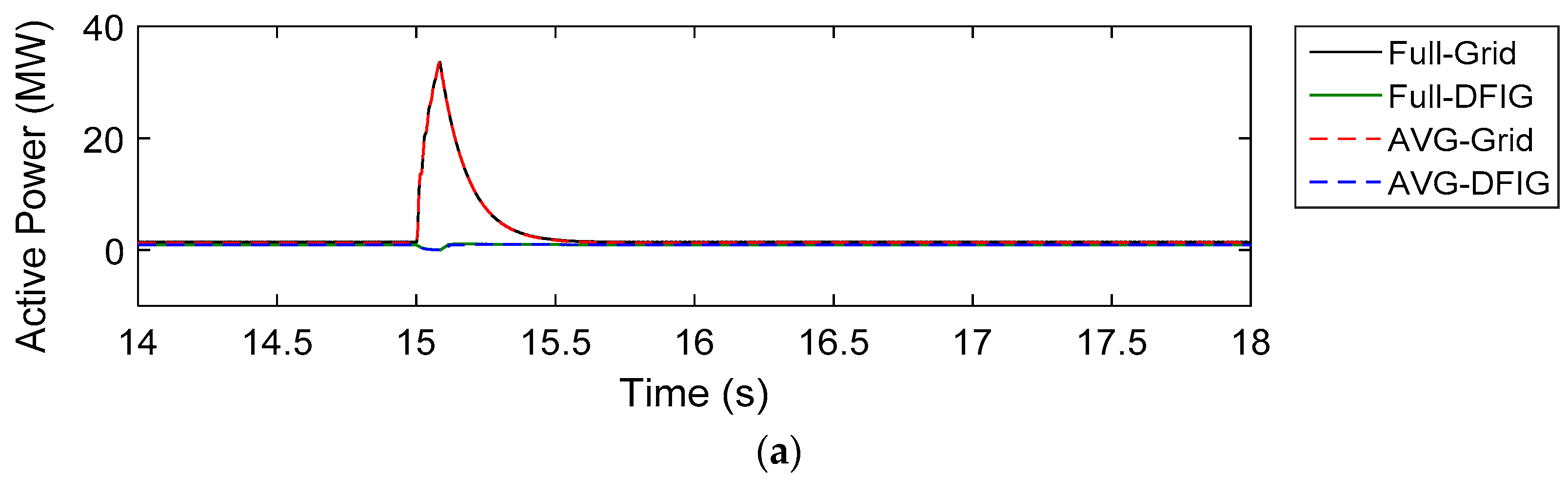
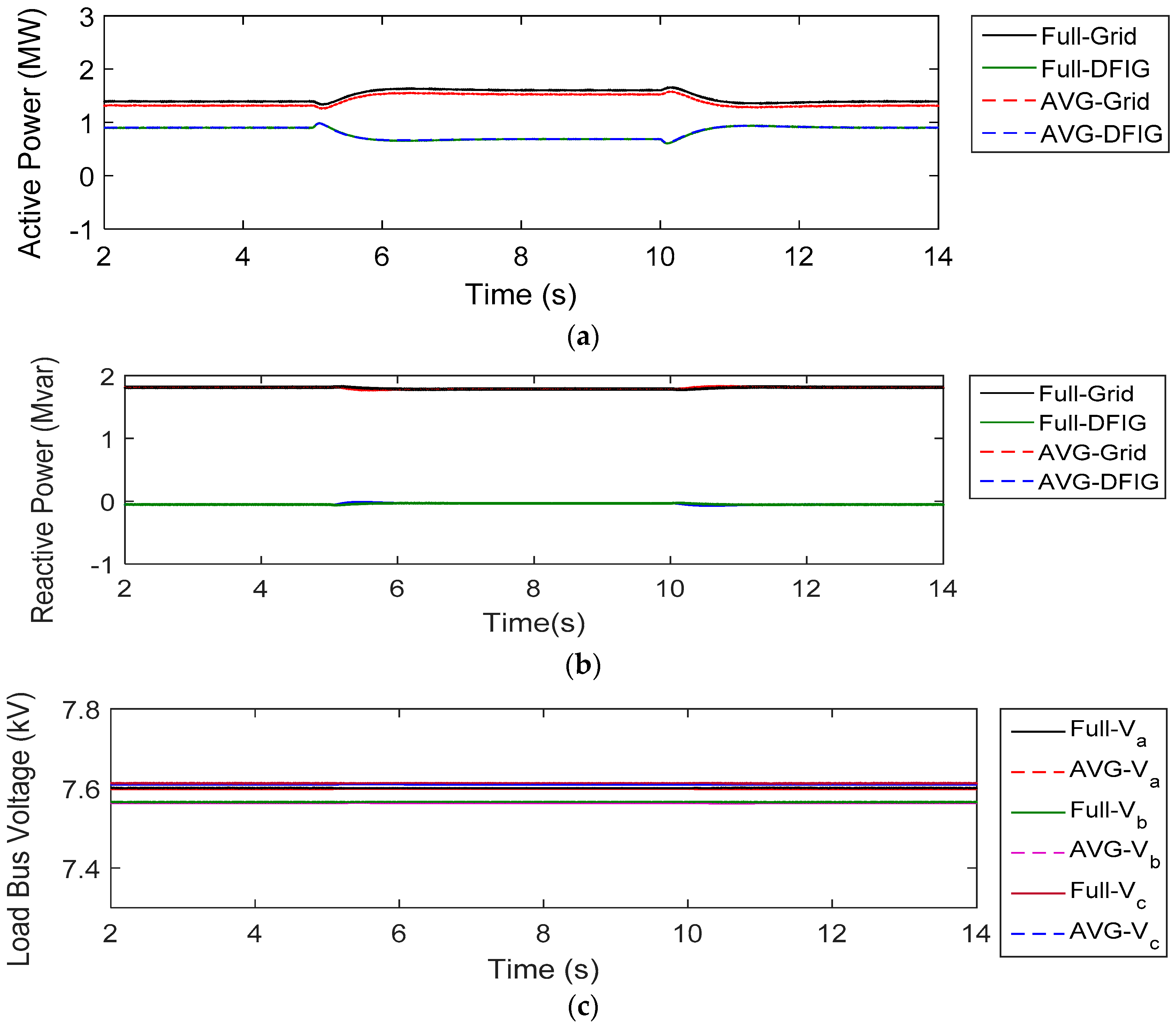
3. Model Validation
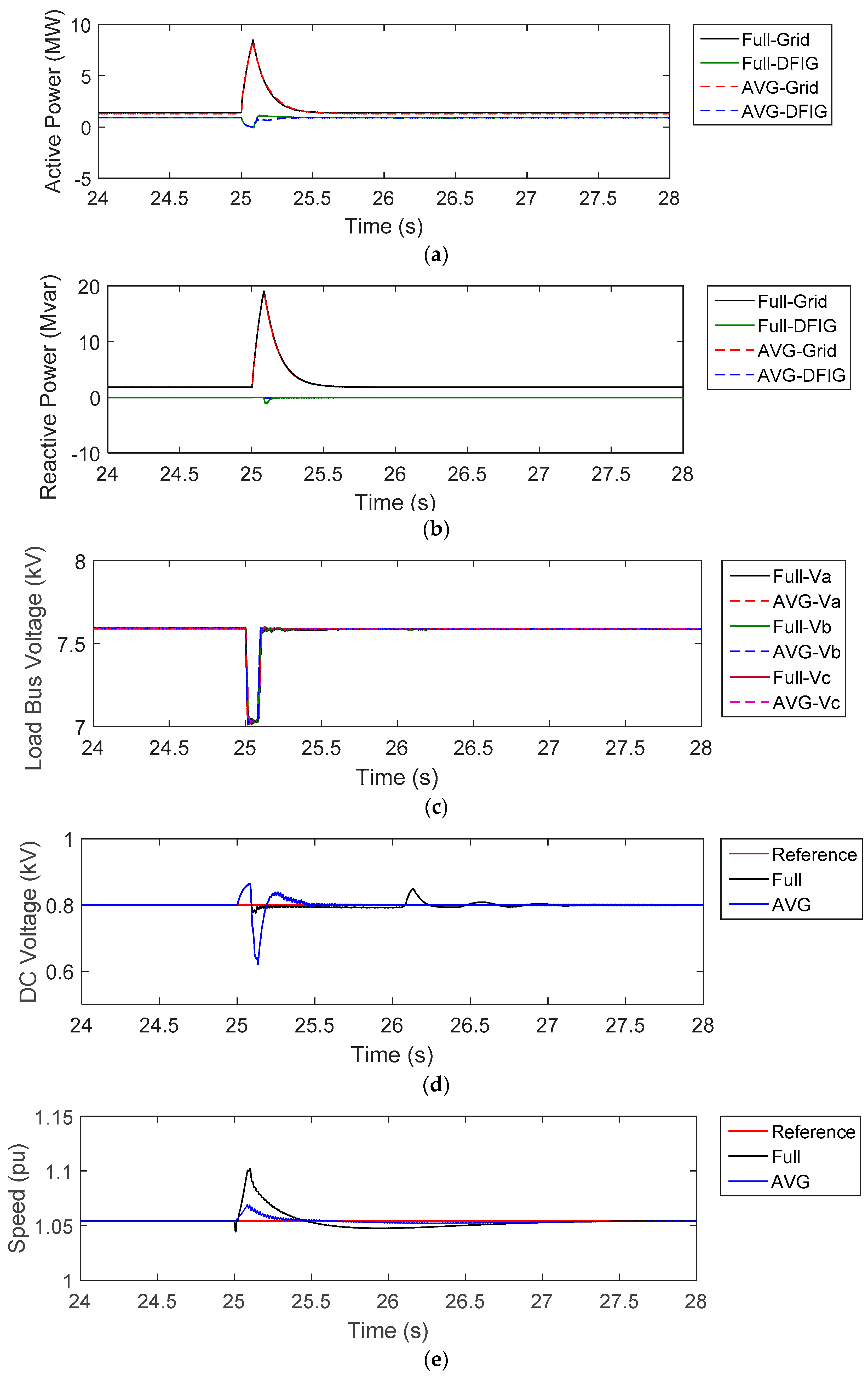
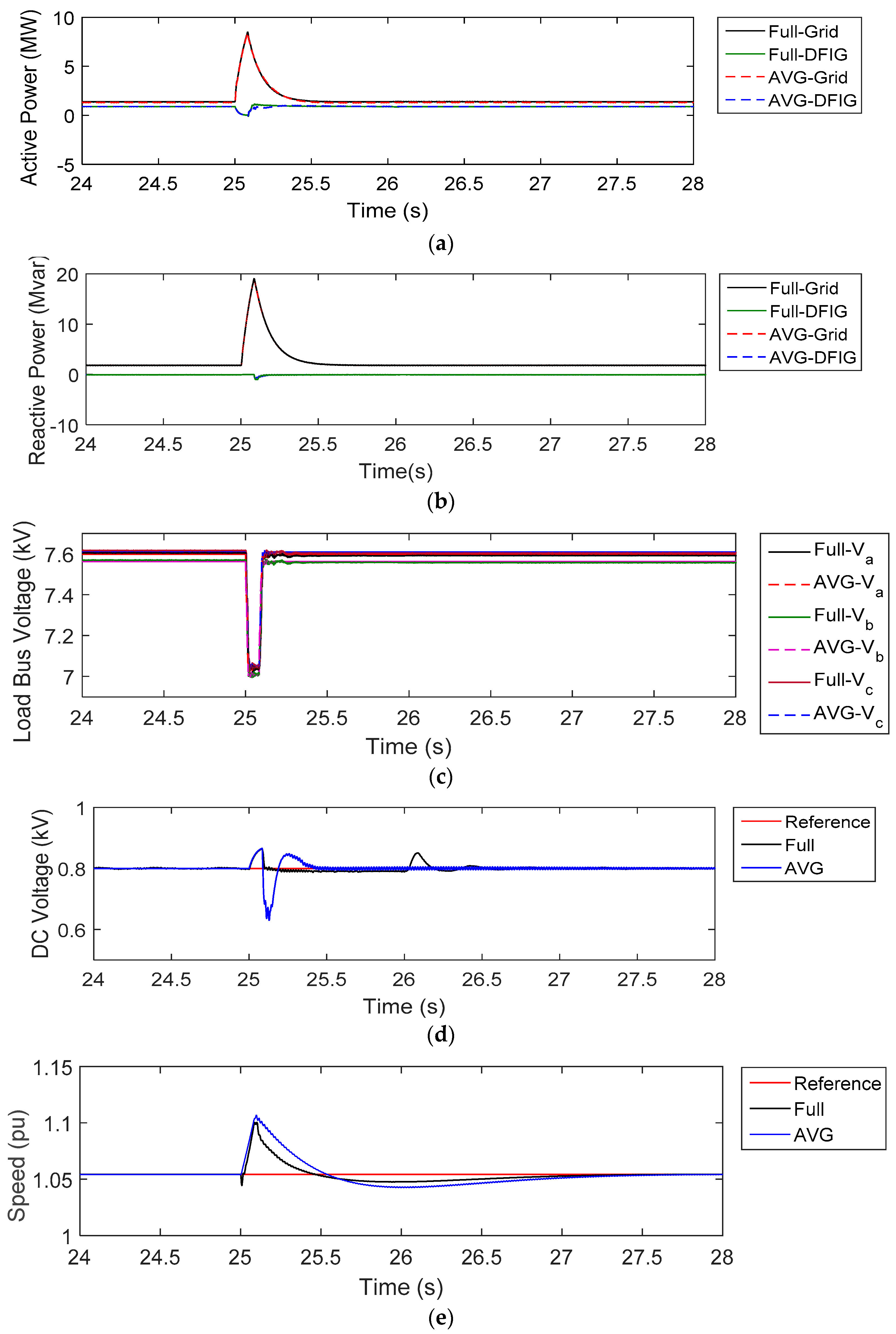
- Scenario 1
- a 3-phase to ground fault of 0.1 Ω at the DFIG terminal.
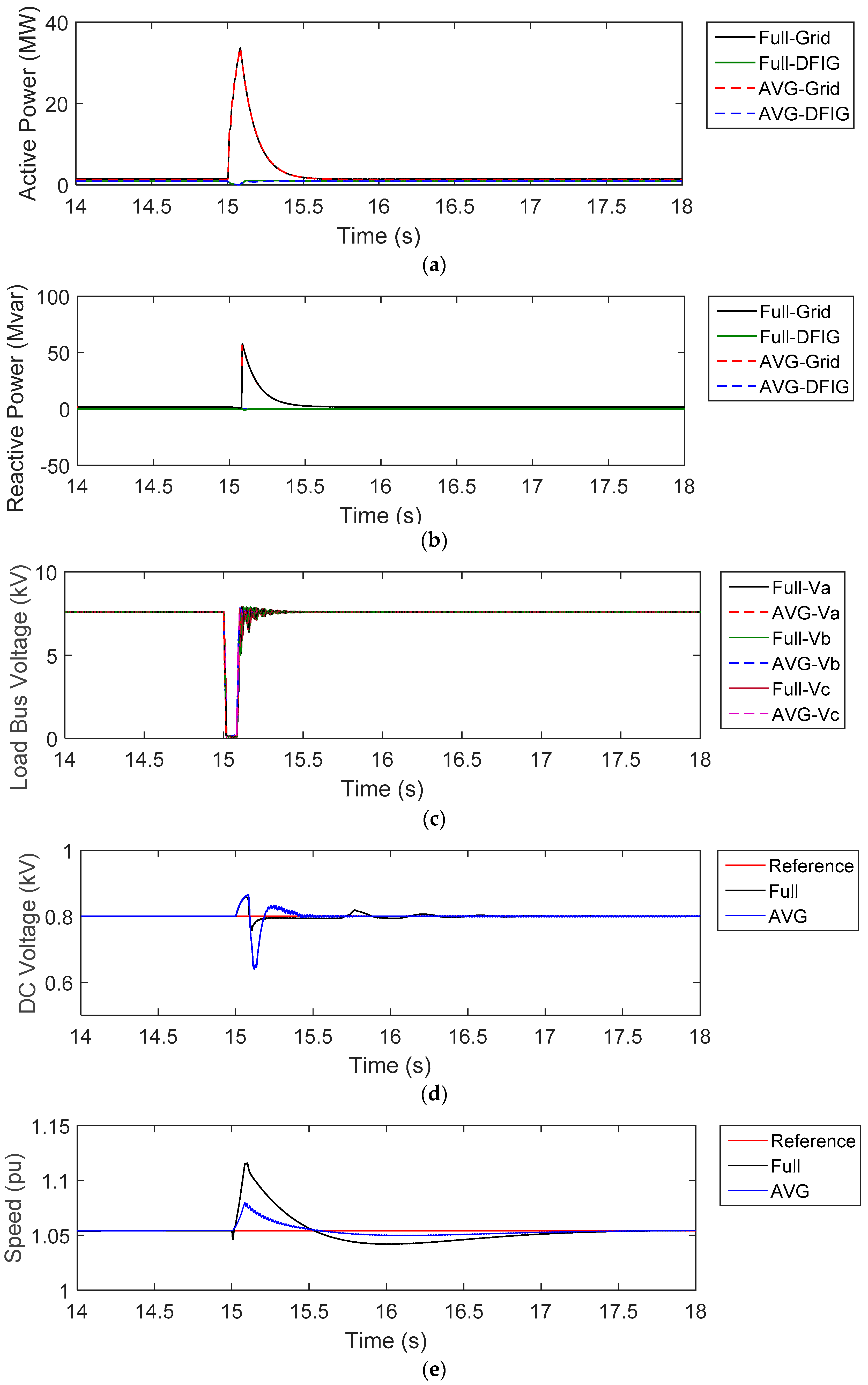
- Scenario 2
- a 3-phase to ground fault of 0.1 Ω at the high voltage (HV) side of the substation transformer.
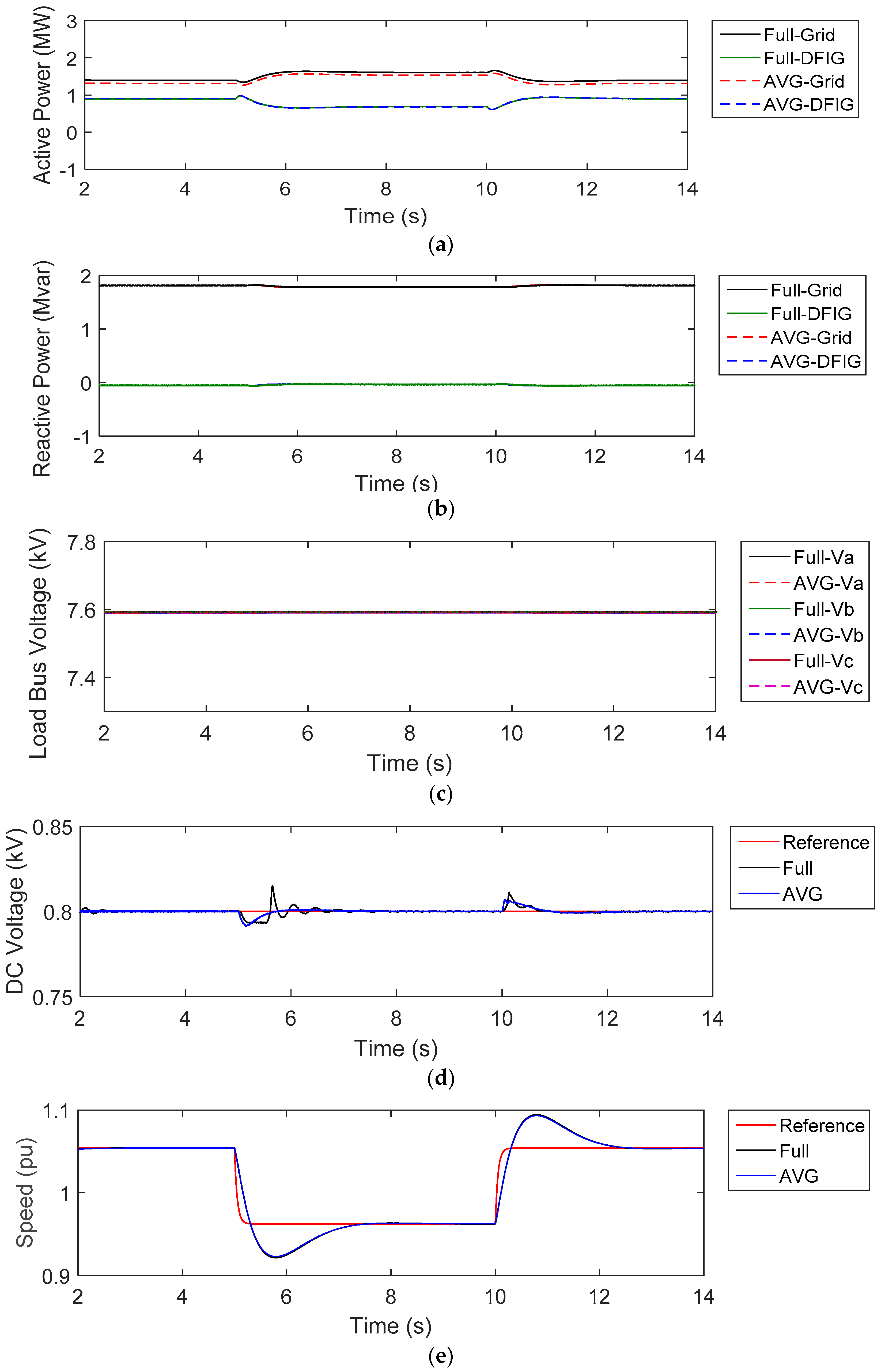
- Scenario 3
- wind speed change from 11.5 ms−1 to 10.5 ms−1 and back to 11.5 ms−1.
3.1. Scenarios 1, 2 and 3 with Balanced Loads
3.2. Scenarios 1, 2 and 3 with Unbalanced Loads
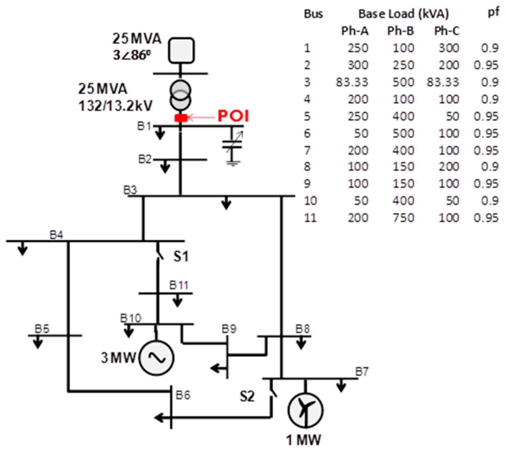
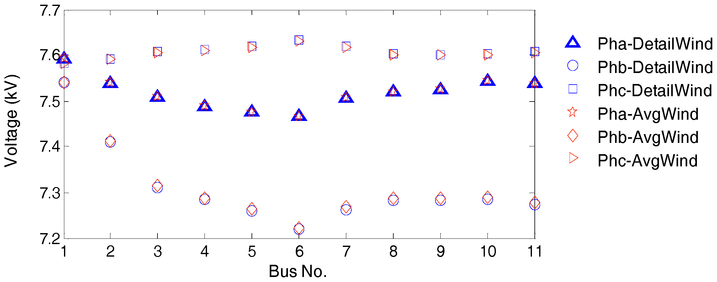
4. Application of DFIG in a Microgrid System
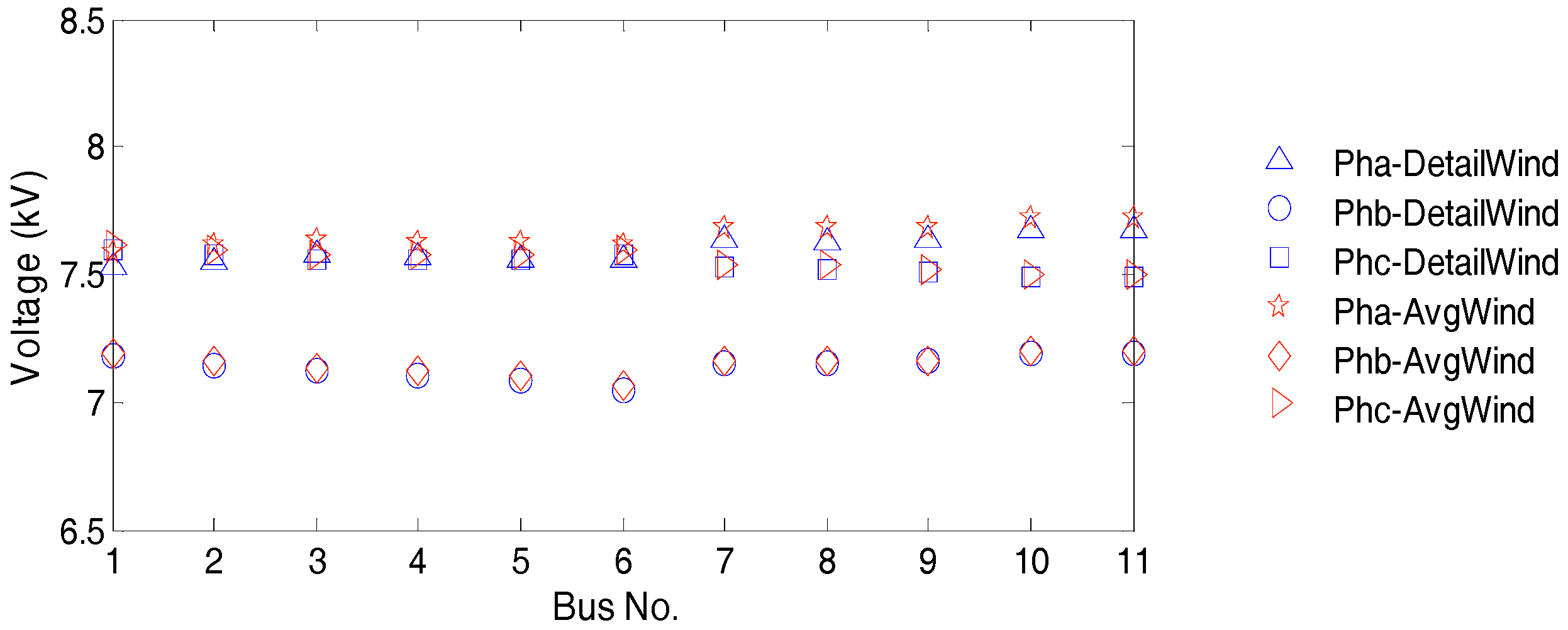
4.1. Steady State Operation of the Microgrid
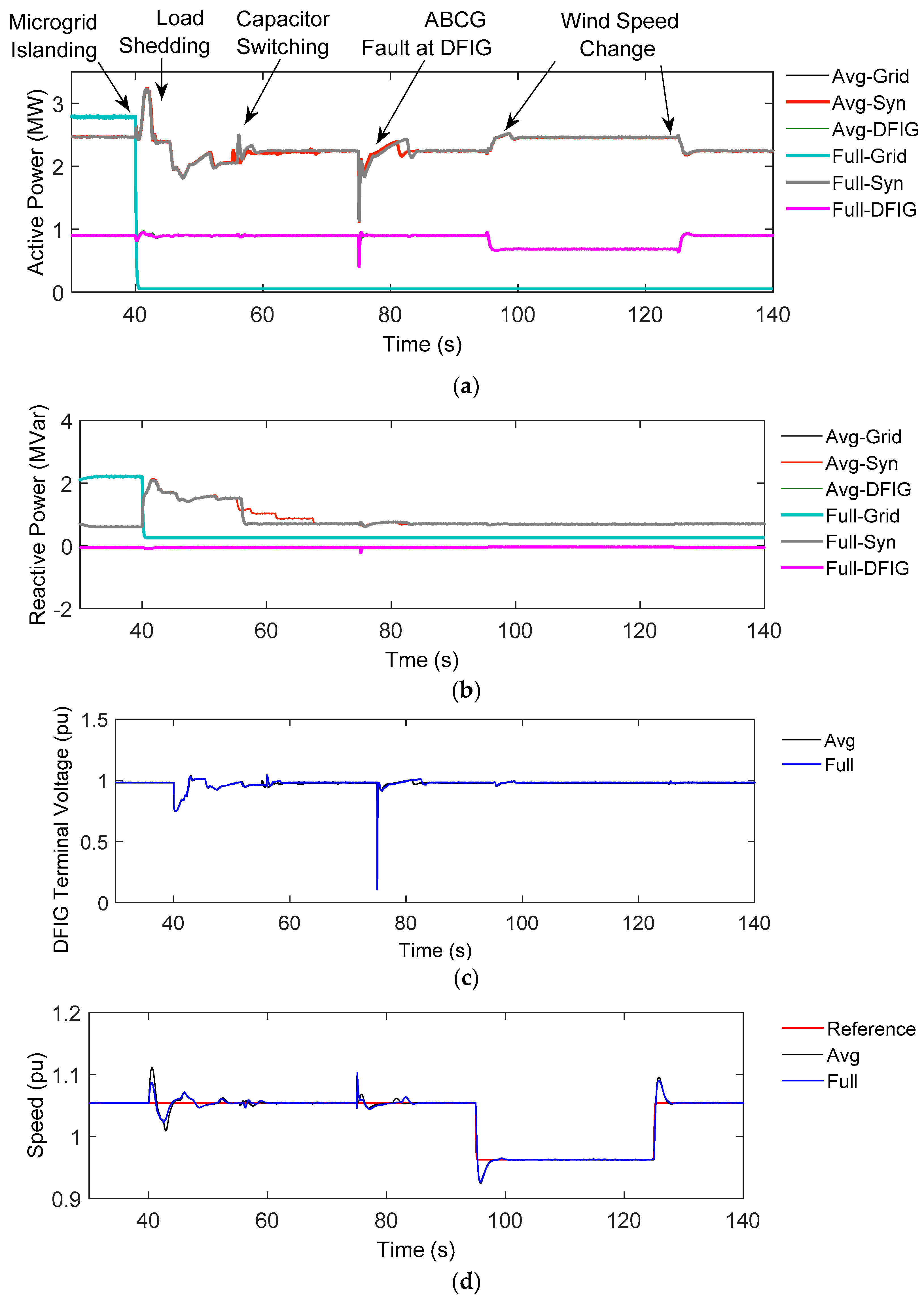
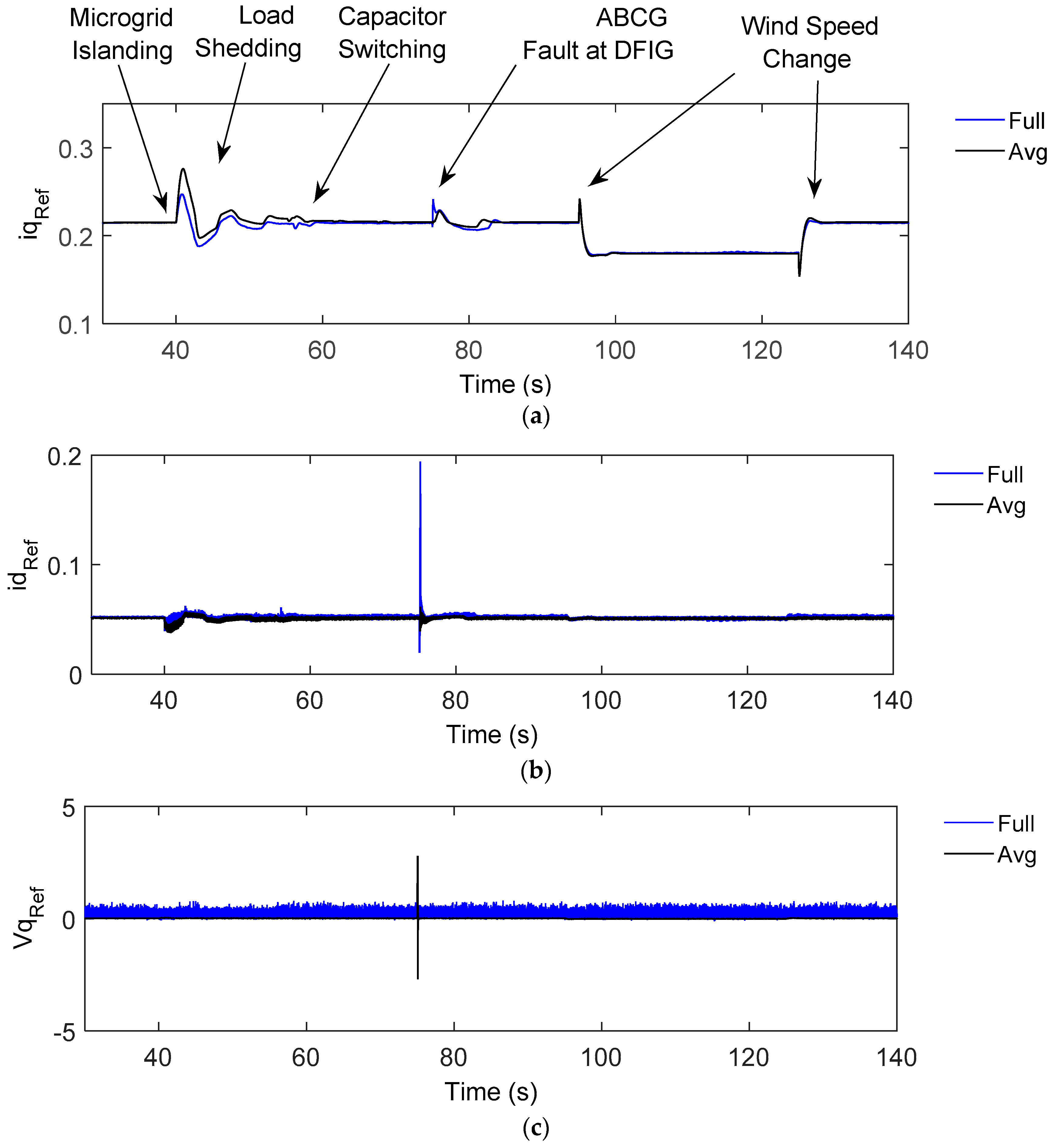
4.2. Transient Operation of the Microgrid
5. Conclusions
Author Contributions
Conflicts of Interest
Appendix A


Appendix B


References
- CanWEA, the Canadian Wind Energy Association. Powering Canada’s Future. 2016. Available online: https://canwea.ca/wp-content/uploads/2017/03/Canada-Current-Installed-Capacity_e.pdf (accessed on 1 October 2017).
- Global Wind Energy Council, Global Wind Report, Annual Marker Update. 2016. Available online: http://gwec.net/publications/global-wind-report-2/global-wind-report-2016/ (accessed on 1 October 2017).
- Li, H.; Chen, Z. Overview of different wind generator systems and their comparisons. IET Renew. Power Gener. 2008, 2, 123–138. [Google Scholar] [CrossRef]
- Zhao, J.; Lyu, X.; Fu, Y.; Hu, X.; Li, F. Coordinated microgrid frequency regulation based on DFIG variable coefficient using virtual inertia and primary frequency control. IEEE Trans. Energy Convers. 2016, 31, 833–845. [Google Scholar] [CrossRef]
- Huang, P.; El Moursi, M.S.; Xiao, W.; Kirtley, J.L. Subsynchronous Resonance Mitigation for Series-Compensated DFIG-Based Wind Farm by Using Two-Degree-of-Freedom Control Strategy. IEEE Trans. Power Syst. 2015, 30, 1442–1454. [Google Scholar] [CrossRef]
- Hosseini, S.H.; Sharifian, M.B.B.; Shahnia, F. Dynamic performance of double fed induction generator for wind turbines. In Proceedings of the Eighth International Conference on Electrical Machines and Systems (ICEMS 2005), Nanjing, China, 27–29 September 2005; Volume 2, pp. 1261–1266. [Google Scholar]
- Ekanayake, J.B.; Holdsworth, L.; Wu, X.; Jenkins, N. Dynamic modeling of doubly fed induction generator wind turbines. IEEE Trans. Power Syst. 2003, 18, 803–809. [Google Scholar] [CrossRef]
- Gagnon, R.; Sybille, G.; Bernard, S.; Paré, D.; Casoria, S.; Larose, C. Modeling and real-time simulation of a doubly-fed induction generator driven by a wind turbine. In Proceedings of the International Conference on Power Systems Transients (IPST’05), Montreal, QC, Canada, 19–23 June 2005. [Google Scholar]
- Ying, J.; Yuan, X.; Hu, J. Inertia Characteristic of DFIG-based WT under Transient Control and Its Impact on the First-Swing Stability of SGs. IEEE Trans. Energy Convers. 2017. [Google Scholar] [CrossRef]
- Wang, Y.; Xu, L.; Williams, B.W. Compensation of network voltage unbalance using doubly fed induction generator-based wind farms. IET Renew. Power Gener. 2009, 3, 12–22. [Google Scholar] [CrossRef]
- Xu, L.; Andersen, B.R.; Cartwright, P. VSC transmission operating under unbalanced AC conditions—Analysis and control design. IEEE Trans. Power Deliv. 2005, 20, 427–434. [Google Scholar] [CrossRef]
- Zhao, C.; Guo, C. Complete-independent control strategy of active and reactive power for vsc based HVDC system. In Proceedings of the IEEE Power & Energy Society General Meeting (PES ’09), Calgary, AB, Canada, 26–30 July 2009; pp. 1–6. [Google Scholar]
- Wu, B.; Lang, Y.; Zargari, N.; Kouro, S. Power Conversion and Control of Wind Energy Systems; The Institute of Electrical and Electronics Engineers; John Wiley & Sons, Inc.: Hoboken, NJ, USA, 2011; pp. 322–323. [Google Scholar]
- WWD-1, Appendix 10-Technical Specification 1, Ver 8-1/2003 Winwind Oy, Elektroniikkatie 2B, FIN-90570 OULU. Available online: http://www.ecosource-energy.bg/uploads/Technical_Specification_WWD1.pdf (accessed on 1 October 2017).
- Lidula, N.W.A.; Rajapakse, A.D. Impact of Islanding Detection Time Duration on the Stable Operation of a Synchronous Generator Controlled Microgrid. Technol. Econ. Smart Grids Sustain. Energy 2017, 2. [Google Scholar] [CrossRef]
- Strunz, K. Developing Benchmark Models for Studying the Integration of Distributed Energy Resources. In Proceedings of the 2006 IEEE Power Engineering Society General Meeting, Montreal, QC, Canada, 18–22 June 2006. [Google Scholar]
- IEEE Working Group. Modelling and Analysis of System Transients Using Digital Programs; Velasco, J.M., Keri, A.J.F., Gole, A.M., Eds.; IEEE Operations Center: Piscataway, NJ, USA, 1999. [Google Scholar]
- Hydro, M. Technical Requirements for Connecting Distributed Recourses to the Manitoba Hydro System; DRG 2003; Revision 2; Manitoba Hydro Electric Board: Winnipeg, MB, Canada, 2010. [Google Scholar]
- Rezaei, E.; Ebrahimi, M.; Tabesh, A. Control of DFIG Wind Power Generators in Unbalanced Microgrids Based on Instantaneous Power Theory. IEEE Trans. Smart Grid 2017, 8, 2278–2286. [Google Scholar] [CrossRef]
- Javan, E.; Darabi, A. A New Control Strategy of DFIG-Based Wind Turbines under Unbalanced Grid Voltage Conditions. In Proceedings of the 2nd Power Electronics, Drive Systems and Technologies Conference, Tehran, Iran, 16–17 February 2011. [Google Scholar]
- Zeeshan, A.; Sinha, S.K. Control of DFIG under unbalanced grid voltage conditions: A literature review. In Proceedings of the 2016 International Conference on Control, Computing, Communication and Materials (ICCCCM), Allahabad, India, 21–22 October 2016. [Google Scholar]
- Lidula, N.W.A.; Rajapakse, A.D. Voltage Balancing & Synchronization of Microgrids. Renew. Sustain. Energy Rev. J. 2014, 31, 907–920. [Google Scholar]


© 2017 by the authors. Licensee MDPI, Basel, Switzerland. This article is an open access article distributed under the terms and conditions of the Creative Commons Attribution (CC BY) license (http://creativecommons.org/licenses/by/4.0/).
Share and Cite
Widanagama Arachchige, L.N.; Rajapakse, A.D.; Muthumuni, D. Implementation, Comparison and Application of an Average Simulation Model of a Wind Turbine Driven Doubly Fed Induction Generator. Energies 2017, 10, 1726. https://doi.org/10.3390/en10111726
Widanagama Arachchige LN, Rajapakse AD, Muthumuni D. Implementation, Comparison and Application of an Average Simulation Model of a Wind Turbine Driven Doubly Fed Induction Generator. Energies. 2017; 10(11):1726. https://doi.org/10.3390/en10111726
Chicago/Turabian StyleWidanagama Arachchige, Lidula N., Athula D. Rajapakse, and Dharshana Muthumuni. 2017. "Implementation, Comparison and Application of an Average Simulation Model of a Wind Turbine Driven Doubly Fed Induction Generator" Energies 10, no. 11: 1726. https://doi.org/10.3390/en10111726
APA StyleWidanagama Arachchige, L. N., Rajapakse, A. D., & Muthumuni, D. (2017). Implementation, Comparison and Application of an Average Simulation Model of a Wind Turbine Driven Doubly Fed Induction Generator. Energies, 10(11), 1726. https://doi.org/10.3390/en10111726