1. Introduction
Currently, the growth of urban populations requires the scaling-up of infrastructure in terms of public utilities (including energy), transport and telecommunications. The development of smart technologies, especially smart meters, can help keep these resources available, reliable and affordable. Indeed, smart cities [
1,
2] offer the possibility of managing infrastructures (energy, water, transport, etc.) and their interactions with consumers differently to improve quality of life and to respect the environment. Within this context, cities and electricity companies are implementing many programs to equip buildings with smart meters. Smart meters now allow hourly or daily readings of consumption and, thus, collect a large amount of data. These data include electricity consumption by individual residential customers and small or medium-sized enterprise (SME) customers. Analyzing such data can help in building decision-making tools for urban stakeholders (electricity companies and urban planners) to allow them to better understand the behaviors associated with electricity consumption. This would help refine strategies for optimizing the energy consumption, enhancing the accuracy of predictive models and making simulation models more reliable. In recent years, many research studies have been conducted on using smart meters data to analyze electricity consumption. A review of the related work in this domain will be provided in the next section.
This work aims at extracting a reduced set of electricity consumption patterns from smart meter data that identify typical user behaviors. It falls within the framework of unsupervised machine learning techniques. The proposed approach is based on a constrained Gaussian Mixture Model that can automatically integrate the day type (Saturday, Sunday or weekday) as a time-dependent input variable. The aim of this approach is to group together the consumers who consume in the same manner during the three types of day and not separately. Each cluster is then characterized by three profiles (Saturday, Sunday and working day) and consumers belonging to a cluster behave in the same way during the three types of day. An alternative approach involving first dividing up the data according to the three types of day, and then fitting a basic mixture model to each data category, could have been used. It is important to mention that such approach is different compared to the one presented in this paper. In fact, for each type of day, typical consumption profiles would be determined in this case. Consequently, a smart meter will belong to three clusters: one for working days, a second for Saturdays and a third for Sundays. Then, instead of our approach, it is not possible to consider anymore the simultaneous view on the three day types. The dataset used in this study was collected by the Commission for Energy Regulation (CER) during a smart meter installation trial and contains the electricity consumption information of residential and small or medium-sized enterprise (SME) smart meters located in Ireland during the year 2010. It also contains the data collected by a survey conducted on all the households. In the first step, our model is applied on the data during one month, where no special days (public holidays) occur. The goal is to identify the behaviors of consumers during this month and link these behaviors to socio-economic characteristics extracted from the survey. Then, the second step is dedicated to studying the evolution of consumer behavior over the months of the year 2010 by using our clustering model. The main contributions of this paper can be summarized as follows:
We aim to cluster consumers into a reduced set of groups based on their electricity smart meter data. Our model automatically considers the day type (weekday, Saturday or Sunday), thus providing three typical consumption patterns for each cluster: one for each day type.
We cross the clustering results with socio-economic information of the consumers studied by the CER survey. This post-analysis may offer insights into the relationships between the socio-economic characteristics of consumers and their electricity consumption.
We investigate the variability of consumer behavior over time by analyzing the changes in clustering results from month to another.
In this paper, even if clustering was performed over two temporal horizons (one month and one year), the aim in both cases was to extract a reduced set of typical clusters, each of which is represented by daily patterns of electricity consumption behaviors.
The paper is organized as follows:
Section 2 presents related work on data mining approaches applied to electricity data.
Section 3 describes the dataset as well as the elementary statistics.
Section 4 details the generative model based on a Gaussian mixture distribution. In
Section 5, an in-depth analysis of the residential clustering results during the month of November is carried out. An evaluation of the model is also performed in this Section.
Section 6 is dedicated to the analysis of the clustering results obtained from the same data after normalization. In
Section 7, we discuss the clustering results after applying our approach to the monthly electricity consumption of consumers during the year 2010. Finally,
Section 8 concludes the paper and provides an outlook for future work.
2. Related Work
Many machine learning studies have been conducted in the energy field. In this section, we specifically focus on studies applied to the electricity consumption of buildings.
A greater number of researchers have used supervised learning methods [
3,
4,
5] to model electrical consumption according to different socio-economic characteristics. Recently, Devijver et al. in [
6] developed a new methodology based on high-dimensional regression models to cluster 4225 households located in Ireland. The authors showed that the obtained clusters could be exploited for profiling as well as for forecasting. In [
7,
8], the authors used another supervised machine learning method to estimate household socio-economic characteristics (e.g., employment and number of children) from the electricity consumption. They also developed a method to determine the sensitivity of household electricity consumption to the times of sunset and sunrise and to the outdoor temperature. Regarding unsupervised frameworks, K-means is one of the most-used clustering methods [
9,
10,
11]. Keeping to the centroid approach, several studies have used Self-Organizing Maps (SOMs) to cluster consumers [
12,
13,
14]. Other data mining techniques such as Density-Based Spatial Clustering of Application with Noise (DBSCAN), the Classification-Regression Tree and Artificial Neural Networks (ANNs) were applied to the same dataset to compare the method’s performance and behavior concerning outliers [
15,
16,
17]. Birt et al., in [
18], by aggregating 327 households in Canada into categories, discovered strong correlations between household electricity consumption and temperature fluctuations in both winter and summer. This approach permits a determination of the electrical consumption caused by heating and cooling. Similar clustering techniques, namely, hierarchical clustering and K-means, were used in [
19,
20] with the goal of identifying household clusters that exhibited the same peak usage times and determining stable household profiles during a certain time period.
Recently, four studies have been proposed and all of them have focused on the same smart grid data we use in this paper [
21,
22,
23,
24]. The first one investigates on three clustering methods: K-means, K-medoid and SOMs and chooses the best performing method to segment individual households into clusters based on their daily electricity consumption. This process is performed over a six-month period; the output is a series of Profile Classes (PCs). Finally, each PC is linked to household features through a multinomial logistic regression. The second paper presents a detailed analysis of smart meter data to understand peak demand and the major sources of consumer variability in terms of behavior. The clustering is based on seven attributes that are computed for each consumer over the period of a year. By using a Finite Mixture Model based on a clustering method, a reduced subset of groups were discovered. In [
23], a study was conducted on smart metering data in order to analyze and identify the link between energy patterns and household information in Ireland. Three clusters of consumers were identified by using the so-called X-means algorithm and labeled as: the day group, the evening group and the midnight group. It was found that energy behavior is primarily correlated with Internet usage. Another approach for clustering the dynamics of electricity consumption behavior has been advanced in [
24]. This approach was applied to 6445 customers, containing 4511 residential customers, 391 industrial customers and 1533 customers whose nature was unknown. This study aimed to identify potential targets for the development of specific programs.
The work presented in this paper shares the same goal as that carried out by the authors of [
25,
26], since we both aim to summarize a large dataset of energy consumption that was collected from a considerable number of meters. The objective is to form a reduced set of typical daily patterns linked to consumer lifestyles. In [
26], the methodology used to create a load-shape dictionary operates in two stages since the authors perform an iterative K-means algorithm followed by hierarchical clustering to merge subclusters, which are too close. Here, we propose to perform the clustering with an extension of the basic Gaussian Mixture Model, which integrates the type of day (Saturday, Sunday and weekday) as a time-dependent input variable. The proposed model aims to group the consumers who consume in the same manner during the three types of day and not separately. The second part of the work presented in the submission focused on changes in consumer behavior over time, which is also quantified on the basis of the entropy. One difference is due to the fact that the dataset used in this study spans only one year and the locations of the consumers are not available. The datasets used in [
25,
26] span longer periods and the locations of meters are known, which is useful information for the clustering model and the interpretation of the results.
In the next section, the data studied in the present article are described.
3. Data and Preprocessing
The studied data concern the electricity consumption of 6445 buildings located in Ireland. This dataset was made available by the Irish Commission for Energy Regulation CER (
http://www.ucd.ie/issda/data/commissionforenergyregulationcer/) within the framework of a smart metering project. Two types of information are provided: the electrical power consumed at each building, which was recorded every 30 min by smart meters during the year 2010, and additional building characteristics, collected via a questionnaire. Among these characteristics are labels that refer to residential buildings (65.55%), small or medium-sized enterprises (SME) (7.52%) and to the category “other” (26.92%), representing the consumers who did not completely answer the questionnaire. In this paper, we focus only on the residential category, which covers more than 4000 smart meters.
Removing the meters with missing values resulted in 2995 electricity consumption time series.
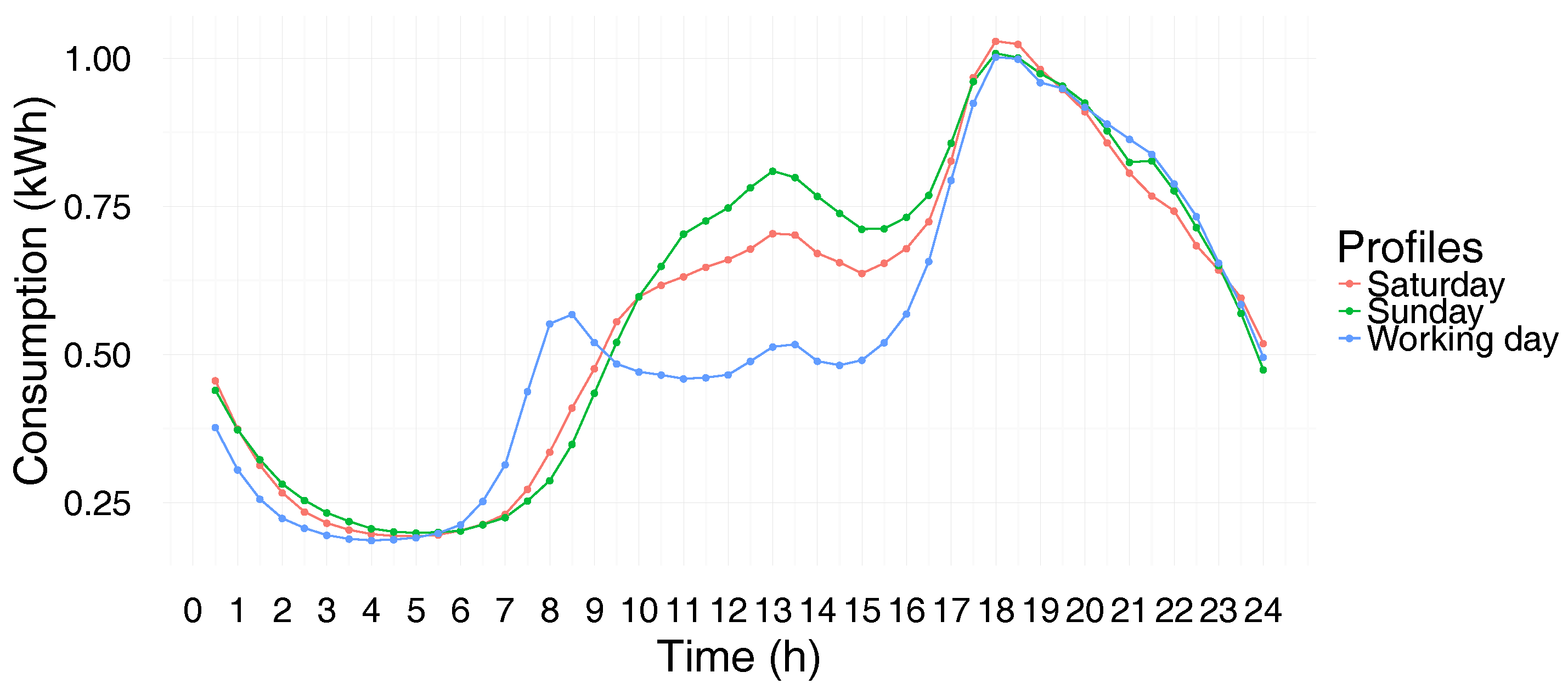
Figure 1 represents the average electricity consumption of the residential buildings for the three day types (Saturday, Sunday and weekday) during a month of the year 2010.
In the remainder of this paper, the following notations will be used. The set of electrical power consumption series to be classified will be denoted as , where is the number of smart meters remaining after the preprocessing steps. The series , which corresponds to the smart meters indexed by i, will be denoted by , where D is the number of days and is the vector of measurements recorded every 30 min. As we have opted to work on monthly periods, the number of days D belongs to the set .
The next section will detail the proposed model as well as the procedures for estimating its parameters.
4. A Constrained Mixture Model-Based Clustering Approach
This section focuses on the identification of the electricity consumption patterns from smart meter data by considering the month of November 2010. A constrained mixture model-based approach that integrates a time-dependent input variable encoding the day type is developed for this purpose.
4.1. Generative Model
The proposed model is a
K-component mixture that assumes that the time series
associated with the smart meters are distributed according to the density
where
is the Gaussian distribution with mean
and covariance matrix
, the
are the proportions of the mixture satisfying
, and
is the set of parameters of the model. The latent variable encoding the cluster membership of the meter
i is denoted by
. Due to the high dimension (
) of the studied time series, it is assumed that the covariance matrices
are diagonal. In this case,
and
can be decomposed as follows:
where the
’s
are
T-dimensional vectors and
is the block-diagonal matrix whose blocks are the
diagonal covariance matrices
.
Unlike the usual mixture modeling approach, which does not impose any additional constraint on the model parameters, the following restrictions are imposed on the model structure:
with
, which corresponds to the day types Saturday
, Sunday
and weekday
, and
and
are, respectively, the
T-dimensional vector and
diagonal covariance matrix corresponding to the day type
l. For the month of November 2010, which starts on a Monday, the mean
and covariance matrix
can be explicitly written as
which highlights that the proposed model requires fewer parameters than the usual Gaussian mixture model. The adopted formalism can be made more general by using the binary variables
(
if
d corresponds to day type
l, and
otherwise). Using these dependent variables and assuming the previously defined constraints, the mixture density defined by Equation (
1) can be re-written as:
Other binary variables could have been used in the proposed model to encode, for example, holidays. In addition, since only one year’s data is available, the estimation of model parameters with such modeling will have limited accuracy (because of the limited number of observed holidays). It should be noted that public holidays have been encoded as Sundays.
In the rest of the paper, it will be assumed that . The parameter estimation procedure is described in detail in the next section.
4.2. Maximum Likelihood Estimation via the EM Algorithm
To estimate the mixture model parameters, the maximum likelihood approach is applied via the Expectation Maximization algorithm [
27]. For the proposed model, the log-likelihood criterion to be maximized is given by:
Before presenting this algorithm, let us define the complete data log-likelihood, which can be written as:
where the variable
equals 1 when
and 0, otherwise.
As is usual in mixture model initialization, a K-means algorithm is used to partition the meters into K clusters. A preliminary estimation of the proposed model parameters is thus provided by the resulting K-means parameters.
Starting from an initial parameter
, the EM algorithm [
27] consists of iterating the following steps until convergence:
Expectation (E step), which consists in evaluating the expectation of the complete log-likelihood conditionally on the observed data
. This quantity is given by:
where
is the posterior probability that meter
i belongs to cluster
k with the current parameters
. This quantity is given by:
Maximization (M step), which consists in maximizing the expectation
Q with respect to
. This maximization leads to the following formulas:
The stopping criterion used in the EM algorithm is based on a predefined log-likelihood threshold. The resulting iterative procedure can be summarized by Algorithm 1. After the algorithm has converged, a partition of the time series into
K clusters is achieved by assigning each time series
to the cluster having the highest posterior probability.
| Algorithm 1: EM algorithm |
![Energies 10 01446 i001]() |
It is worth noting that the proposed approach differs from that consisting in first dividing the data into
L subsets
of daily consumption time series, with
and then separately classifying each of these subgroups using the basic Gaussian mixture model approach. The main difference is that the latter does not directly lead to a partition of
but rather to a partition of the daily time series
. Let
and
denote, respectively, the sets of daily prototypes and partitions obtained by this method, with
and
, where
is the
T-dimensional daily profile corresponding to the
kth cluster of
,
is the cluster label of the
jth time series of
, and
is the cardinal number
. Partitions
can be rearranged into a single partition
consisting of
clusters, where the cluster labels
result from this reorganization.
In order to group together the consumers who consume in the same manner during the
L day types, additional steps are required. One can, for example, match the set of profiles
to get the desired representation of clusters, or partition the categorical time series defined by the rows of matrix
using a suitable method. Despite the relevance of this scheme, we have opted for a global model in which the temporal aspect is taken into account through a specific structure imposed on the model parameters.
5. Clustering during the Month of November
In this section, the residential data are analyzed during the month of November. The appropriate number of clusters is first assessed. Then, the time series are classified based on the found number of clusters, and the results are quantitatively evaluated and interpreted.
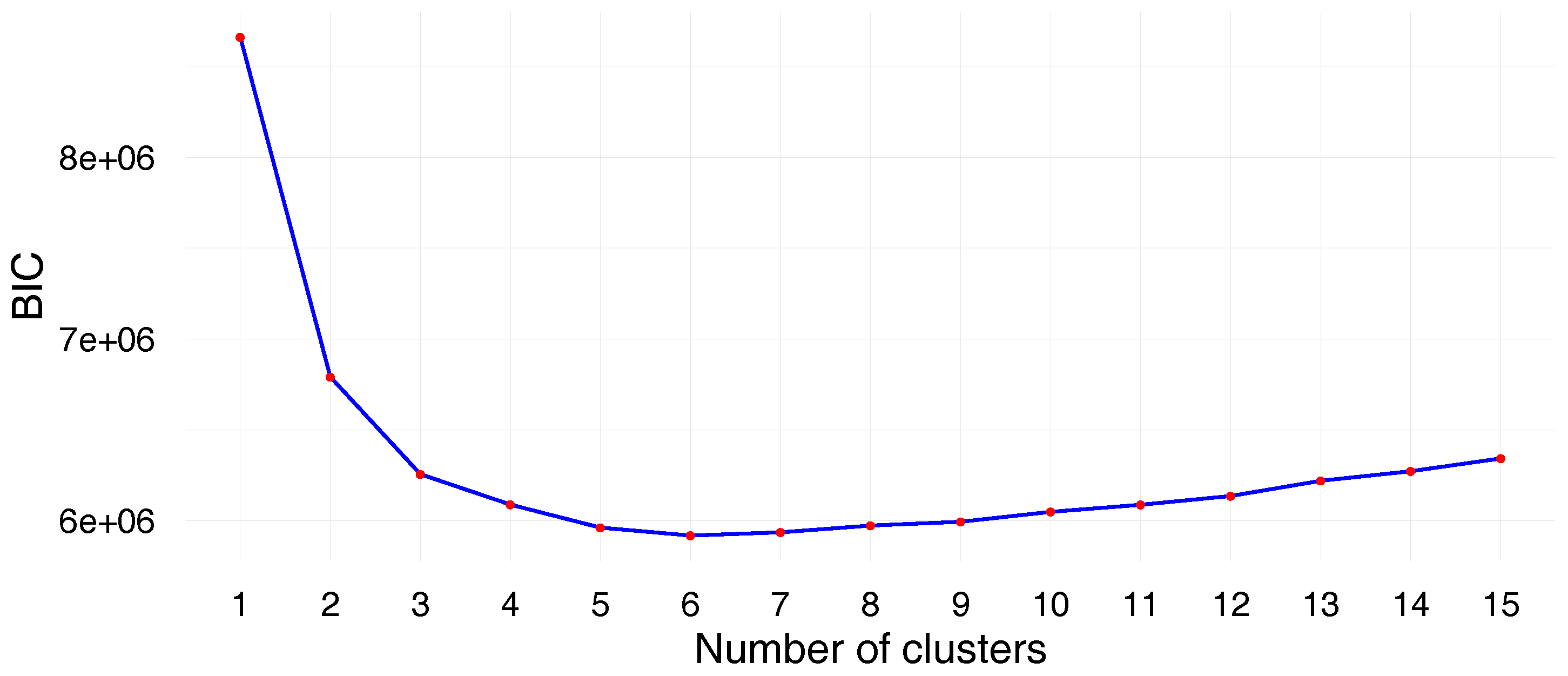
5.1. Choosing the Number of Clusters
To select the number of clusters, the Bayesian Information Criterion (BIC) [
28] is used. This criterion is defined by the likelihood of an item belonging to a cluster penalized by a term that depends on the number of parameters. The BIC criterion is defined by
, where
is the parameter estimated by the EM algorithm and
is the number of parameters. For the proposed
K-component mixture model, we have
.
Figure 2 represents the evolution of BIC according to the number of clusters. It can be noted that BIC decreases until
and then increases progressively. Therefore, we opted for
clusters.
5.2. Evaluation of the Proposed Algorithm
To evaluate the performance of our model, two indicators have been used to better characterize the clusters: the Kullback–Leibler divergence between cluster densities and the proportion of each cluster (see
Table 1). We use the symmetric version of this divergence which is given by:
In this study, we have chosen to assign a label to each cluster depending on its consumption level: the smaller the cluster label is, the less important the average electricity consumption by that clusters is. To measure the size of clusters in relation to the data as a whole, the proportion of each cluster is computed. It can be noted that the proportions of the clusters 2, 3, 4 and 5 are over
; therefore, it is the half for the remaining clusters 1 and 6 (see
Table 1). Since the Kullback–Leibler divergence measures the dissimilarity between cluster densities, the greater the divergence, the more distant the cluster densities are. The values of the closest and most distant cluster densities are shown in bold font in
Table 1. It should be noted that some clusters have a close distribution—for example, clusters (2 and 3) and (4 and 5). In contrast, some clusters such as 1 and 6 are distant.
A comparison is also carried out with a classical clustering algorithms namely: K-means [
29], Hierarchical Ascendant Classification (HAC) [
30] and Basic Gaussian Mixture Model (Basic-GMM) [
27]. This comparison is based on the intra-class inertia, computational time and number of parameters to be estimated for each method. The intra-class inertia is defined by
with
, where
is the
kth cluster center. This criterion estimates the concentration of the series
around the cluster’s center. The smaller the criterion
is, the less dispersed the points are around their cluster center and then the clustering is better. To make the results comparable for all methods, the cluster centers
obtained with K-means, HAC and Basic-GMM have been aggregated under the form of Equation (
4), with
.
Table 2 shows that the proposed method outperforms the K-means, HAC and Basic-GMM algorithms, achieving an improvement of
over the results provided by the two first clustering algorithms and
compared to the Basic-GMM algorithm. The experiments were conducted by using R language (version 3.3.2, GNU project, Auckland University, New Zealand) on a standard PC with an Intel (R) Core (TM) i5 CPU @ 1.80 GHZ processor and 8 GB of RAM. Computational time is longer than with the K-means algorithm, but shorter than with HAC and Basic-GMM. Concerning the number of parameters, since our proposed model is parsimonious, the number of parameters to be estimated is lower than with K-means and Basic-GMM. As a reminder, the number of parameters for our model is computed by
, whereas for K-means
and for Basic-GMM
. As far as HAC is concerned, the concept of parameters is not defined. For a better understanding of consumer electricity behaviors, the next section focuses on the interpretation of the clustering results.
5.3. Interpretation of the Clustering Results
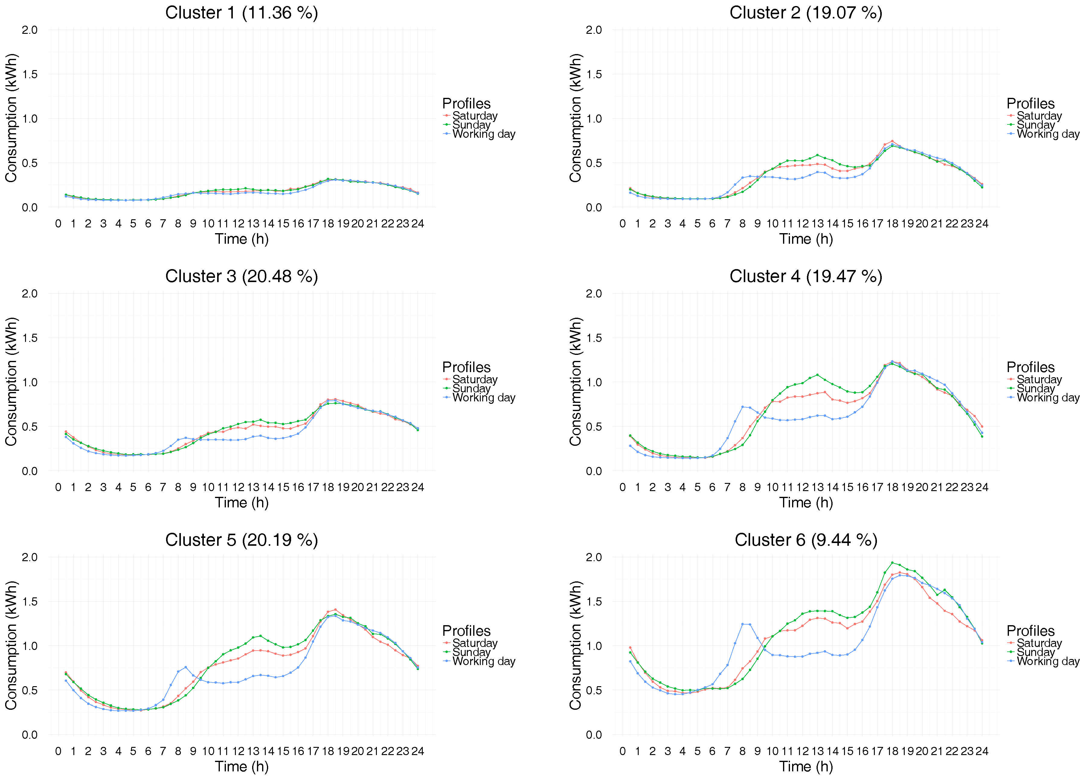
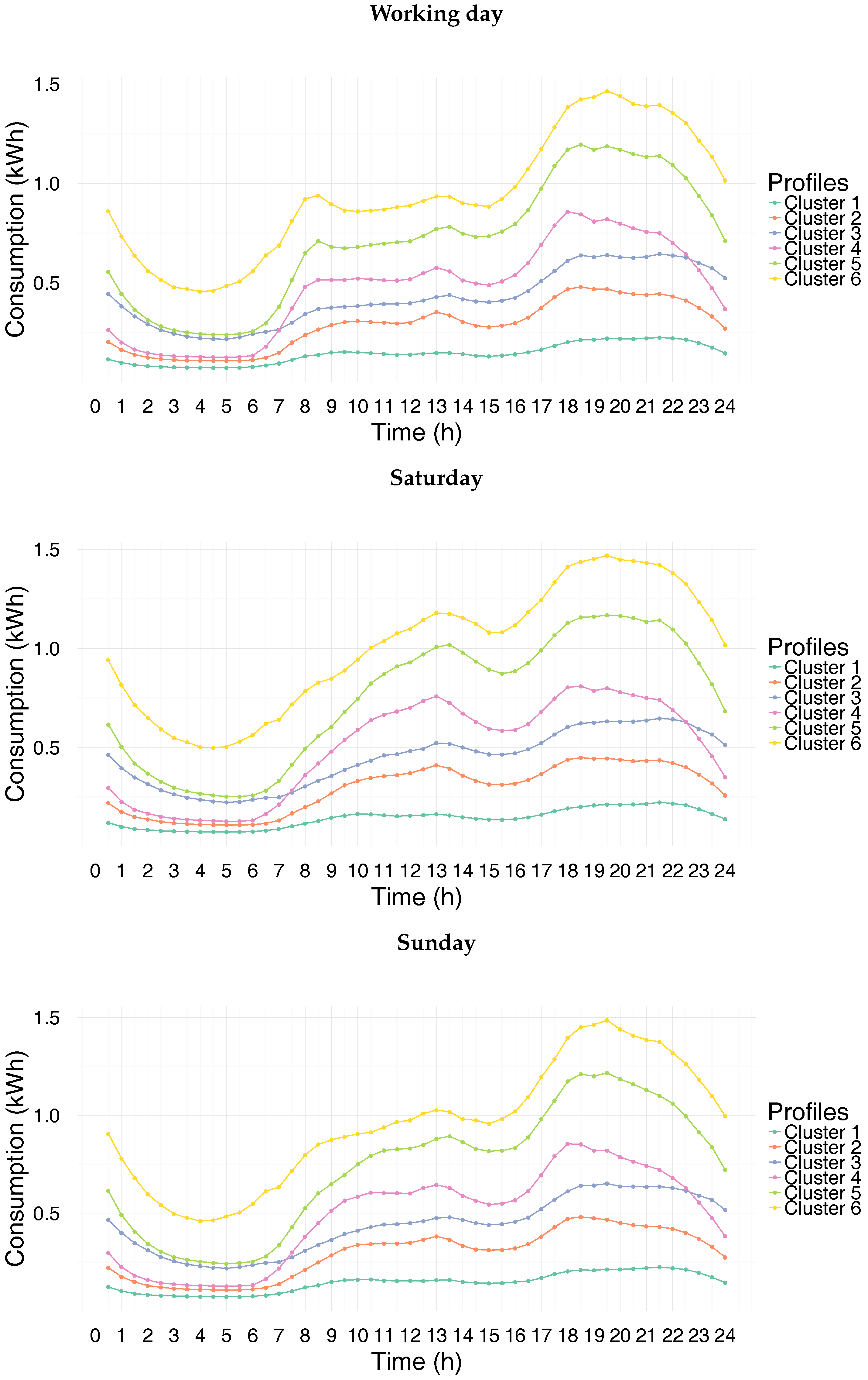
The cluster consumption profiles obtained with the proposed approach
are displayed in
Figure 3. We have chosen to assign a label to each cluster depending on its consumption level. At first glance, four types of electricity consumption patterns can be distinguished:
Cluster 1 is mainly characterized by low consumption load profile. The pattern seems to be similar during both weekdays and weekend days.
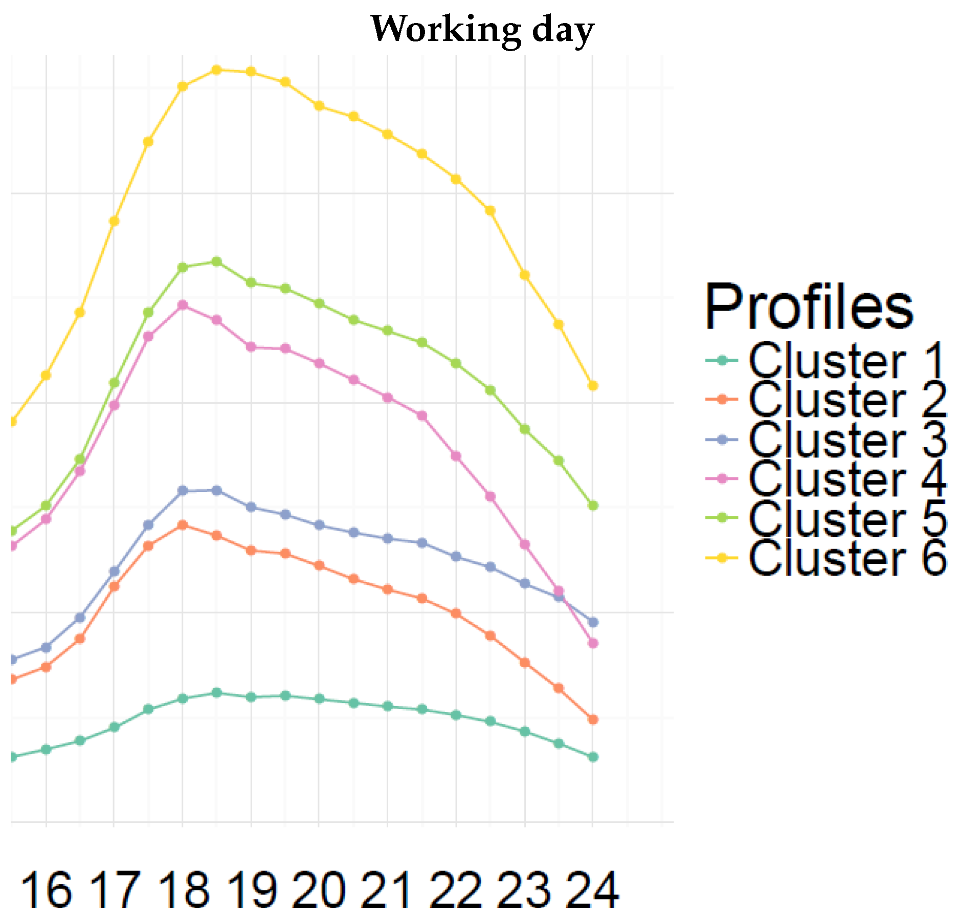
Clusters 2 and 3 are characterized by a relatively low consumption level with a morning peak during weekdays. These peaks are not striking, and they are followed by a small decline. This attests that a minority of the residents in these households leave home during the day. Lunch and evening times are also observable. It can be noted that the two clusters differ mainly in their evening behavior for the time period between 6 p.m. and midnight (see
Figure 4).
Clusters 4 and 5 exhibit a remarkable electricity consumption peak during weekday mornings. The significant gap between the morning peak value and the consumption level after the drop is linked to the number of occupants in the household. For these clusters, a slight increase of the electricity consumption during the lunch time can also be observed. In the evening, their electricity consumption increases to reach a peak. Here, also, the evening behaviors are different for the two clusters for the time period between 6 p.m. and midnight (see
Figure 4).
The behavior of cluster 6 is quite similar to those of the clusters 4 and 5 in spite of the fact that its consumption level is higher.
A similar analysis can be made for weekend days. As can be expected, the electricity consumption shows temporal patterns for weekends different from those of weekdays except for cluster 1. Moreover, the electricity consumption level on Sunday is higher than on Saturday for the time period between 10.30 a.m. and 4.30 p.m. Focusing on clusters 5 and 6, the electricity consumption on Saturday is smaller than that on Sunday between 7.30 p.m. and 11.30 p.m., which can be explained by the fact that occupants belonging to these clusters are more likely to be away from home on Saturday night than on Sunday night.
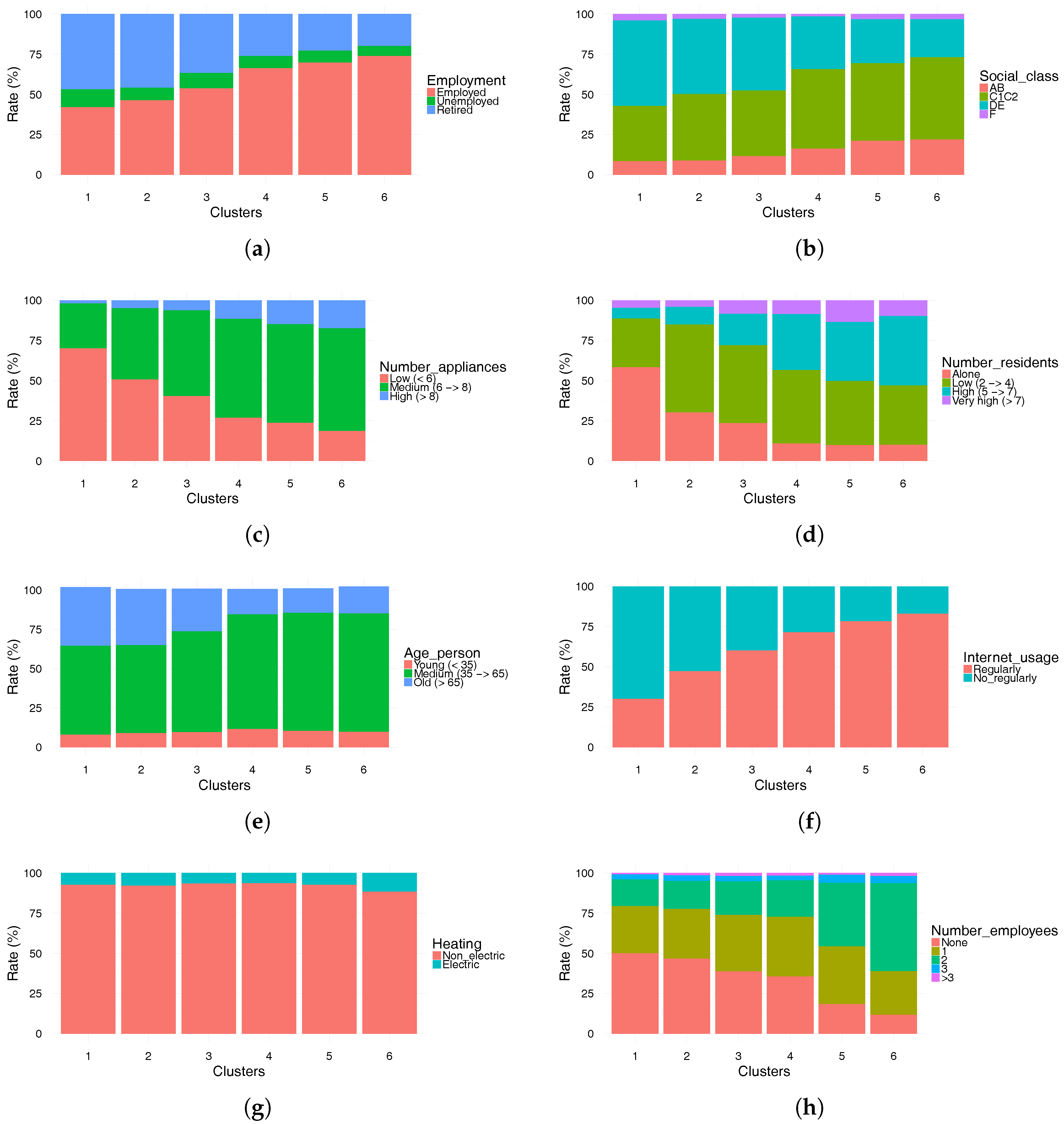
The above observations highlight the close links of temporal patterns of electricity consumption with household residents and their daily lives. A quantitative assessment of these observations can be made by crossing the clustering results with the categorical variables extracted from the residential questionnaires. The choice of the relevant questions is based on the previous work, in particular those presented in [
7,
23]. The authors in [
7] have selected the characteristics that are interesting for utilities by conducting interviews with four energy consultants [
31].
Figure 5 shows the crossing of the clustering results with eight socio-economic characteristics. Unemployed residents (
Figure 5a), as well as alone residents (
Figure 5d), are less important in clusters that exhibit a specific pattern with three distinct and significant rush peaks in the mornings, at lunch time and in the evenings (clusters 4, 5 and 6). These clusters are also characterized by a high percentage of high social class residents compared to clusters 1, 2 and 3, as shown in
Figure 5b. Four modalities are used for this variable, namely, managerial or professional background (AB), intermediate background (C1C2), routine or manual background (DE) and farmers (F). Moreover, it can be noted that the number of retired is slightly more important in cluster 1, where the peak hours of electricity consumption are diffuse and the difference in electricity usage between weekdays and weekends is not significant. It is remarkable that the majority of consumers in all clusters use non-electric means of heating as shown in
Figure 5g. Differences in electricity consumption behaviors also depend on the age of the residents, as shown in
Figure 5e. In particular, the percentage of older people is higher in clusters 1 and 2. Age also has an impact on the use of certain new technologies such as the Internet (see
Figure 5f). Indeed, the majority of consumers in clusters 4, 5 and 6 use the Internet on a regular basis. It can be observed that clusters 4, 5 and 6 with a striking peak in the morning have a higher proportion of employees compared to the other clusters, as shown in
Figure 5h. Finally, these patterns obviously depend on the size of the household, which has a direct impact on the number of electrical appliances it owns. All these observations confirm that accurate electricity consumption profiles reflecting the lifestyles of citizens can be deduced from the available socioeconomic characteristics of the household. Such profiles can be implemented in the simulation models used for smart cities.
6. Clustering Applied to the Normalized Data for the Month of November
This section is concerned with the impact of data normalization on the clustering of consumers. Two types of normalization have been applied, namely centered and reduced standardization, and range normalization. We consider that an electricity consumption behavior is defined only by a habit (shape of curve) and not by the level of consumption.
6.1. Data Normalization
Two types of normalization are applied to the daily electricity consumption
of each consumer
. The first type is centered and reduced standardization. This transforms the values of the vector
with the aim of obtaining the mean and variance of daily electricity consumption equal to 0 and 1, respectively, as shown in below:
where
and
, respectively, denote the raw and normalized electricity consumption during a day
d at time
t.
and
represent the mean and standard deviation of the daily electricity consumption
, respectively.
The second type of standardization is the one suggested in [
24] who used the same Irish data set. It consists of transforming the values of the vector
to the range of
as the following:
where
and
denote the minimum and maximum electricity consumption over a day
d, respectively.
6.2. Interpretation of the Clustering Results
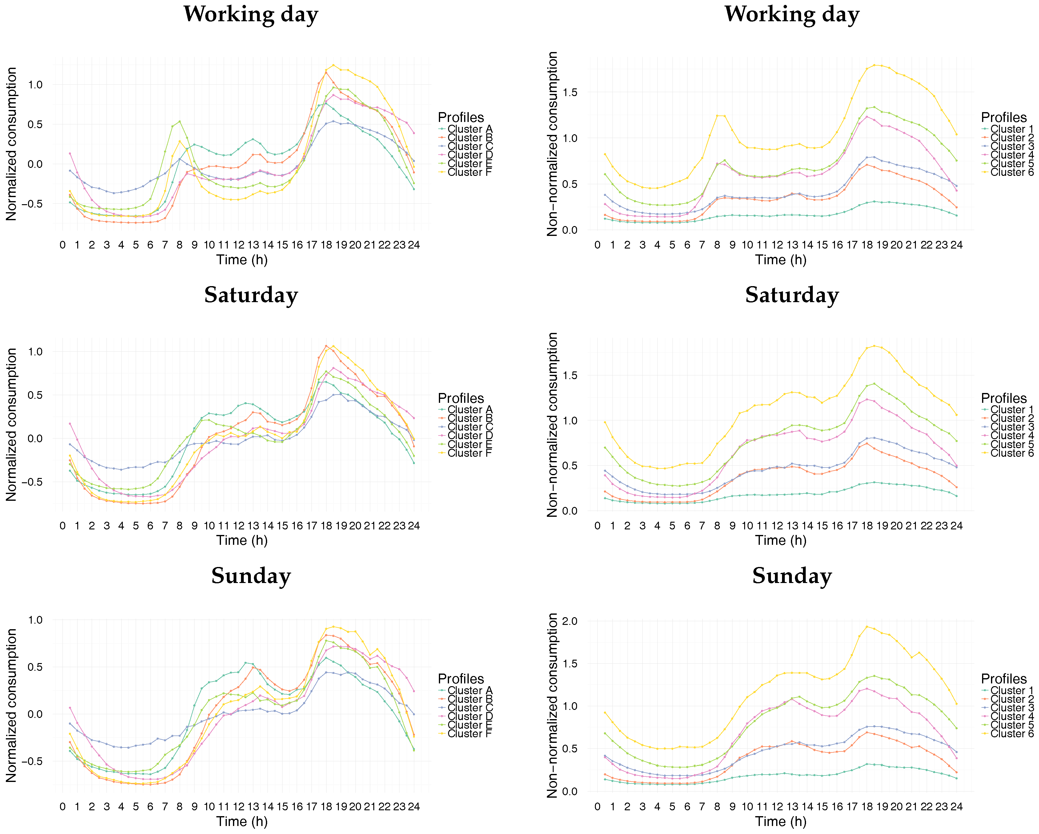
When we applied our proposed model-based approach to the normalized data with the number of clusters set at 6, the curves obtained from the normalized and non-normalized data were quite similar in shape. In this study, we will only consider the results obtained from the centered and reduced normalization data.
Figure 6 represents the electricity consumption profiles from the normalized and non-normalized data. Quantification of the difference between the clustering results obtained with and without normalization can be performed as shown in
Table 3. Each raw result represents the distribution of the consumers in a non-normalized cluster over the six normalized ones (A, B, C, D, E and F). We can observe some remarkable trends. For instance, more than 38% of the population in cluster 1 are present in cluster C. Similar tendencies are highlighted by the transition percentages, which are in bold font. The decision whether or not to perform normalization for the clustering of consumers very much depends on the goal that is targeted. Combining the results with and without normalization would help to target in a precise manner consumers who exhibit certain characteristics in terms of the shape of the peaks in their consumption pattern curves and levels of consumption (in the case of non-normalized data). This can be valuable information for the application of a demand response program [
32].
7. Residential Behavior Changes over Months
In this section, we are interested in studying the evolution of consumer electricity consumption behavior by month in 2010. This investigation helps in understanding the variability in electricity consumption during the year. This work can be helpful to electricity utilities in identifying consumers, who should be targeted with electricity saving solutions such as demand response.
7.1. Methodology
To study the residential behavior changes by month in 2010, our proposed clustering approach is applied to a special data structure consisting of
time series
, where
N is the number of smart meters (2995 smart meters) and
M is the number of months (12 months). This formulation enables a smart meter to change its cluster from one month to another. In fact, the ID of a given smart meter changes across months, thus allowing differentiation between monthly consumption over the year. Here, we have chosen the month as the basic temporal scale. Nevertheless, this decision could be the subject of further investigations. An alternative would be to choose the day as the basic scale. In this study, each time series
represents the electricity consumption of a consumer
i for one month
m. The length of each
is
, where
T is the number of daily measurements (48 measurements) and
is the number of days during month
m. To adapt our model to these data, we use the binary variables
, where
when
and 0, otherwise. The updated formulas for this model are shown in the
Appendix A.
It can be noted that, since the clustering is performed over the year, the obtained daily patterns that are obtained reflect the averaged behavior of the consumers during the year. To reach a more accurate description of the daily patterns during the year, we would need to incorporate additional information about the season as well as public and school holidays. Consequently, this would require datasets covering longer periods in order to estimate the model parameters.
In this analysis, the number of clusters has been set to
in accordance with the Bayesian Information Criterion. As discussed earlier in
Section 5.3, we have chosen to assign a label to each cluster depending on its consumption level.
Figure 7 represents the electricity consumption profiles obtained from the yearly clustering.
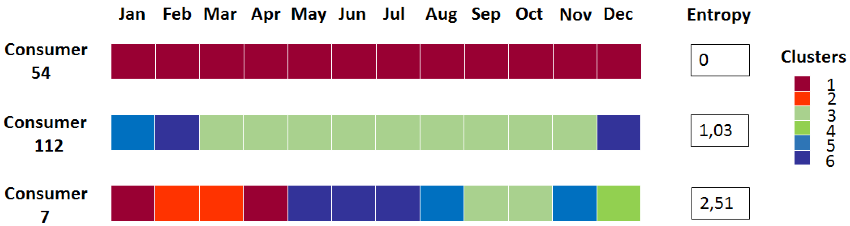
The variability in the behavior of each customer over the months in 2010 has been evaluated using the entropy:
with
, where the
are the
posterior probabilities that customer
belongs to clusters
during months
. The result of this analysis is useful for providing an idea on the evolution of consumer electricity consumption over 2010.
7.2. Discussion
In this part of the study, we do not target individual consumer behaviors but rather the evolution of those behaviors over the months of 2010.
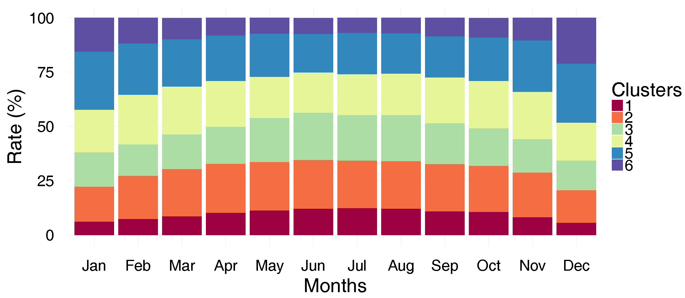
Figure 8 shows the cluster distributions by month. Noticeably, the proportions of clusters 1, 2, 3 and 4 increase from January to June, whereas the proportions of clusters 5 and 6 decrease. Furthermore, the proportions of all clusters are stable between June and August. Conversely, from September until December, the proportions of the clusters 1, 2, 3 and 4 decline, while clusters 5 and 6 show an increase. To better understand these changes in the clusters’ proportions over the months,
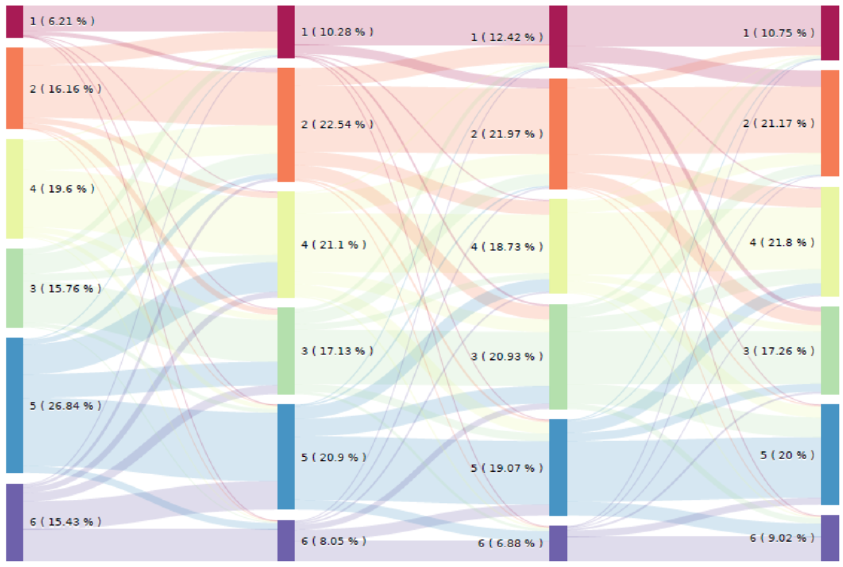
Figure 9 depicts the evolution of the consumer behavior from one cluster to another over the months. To make
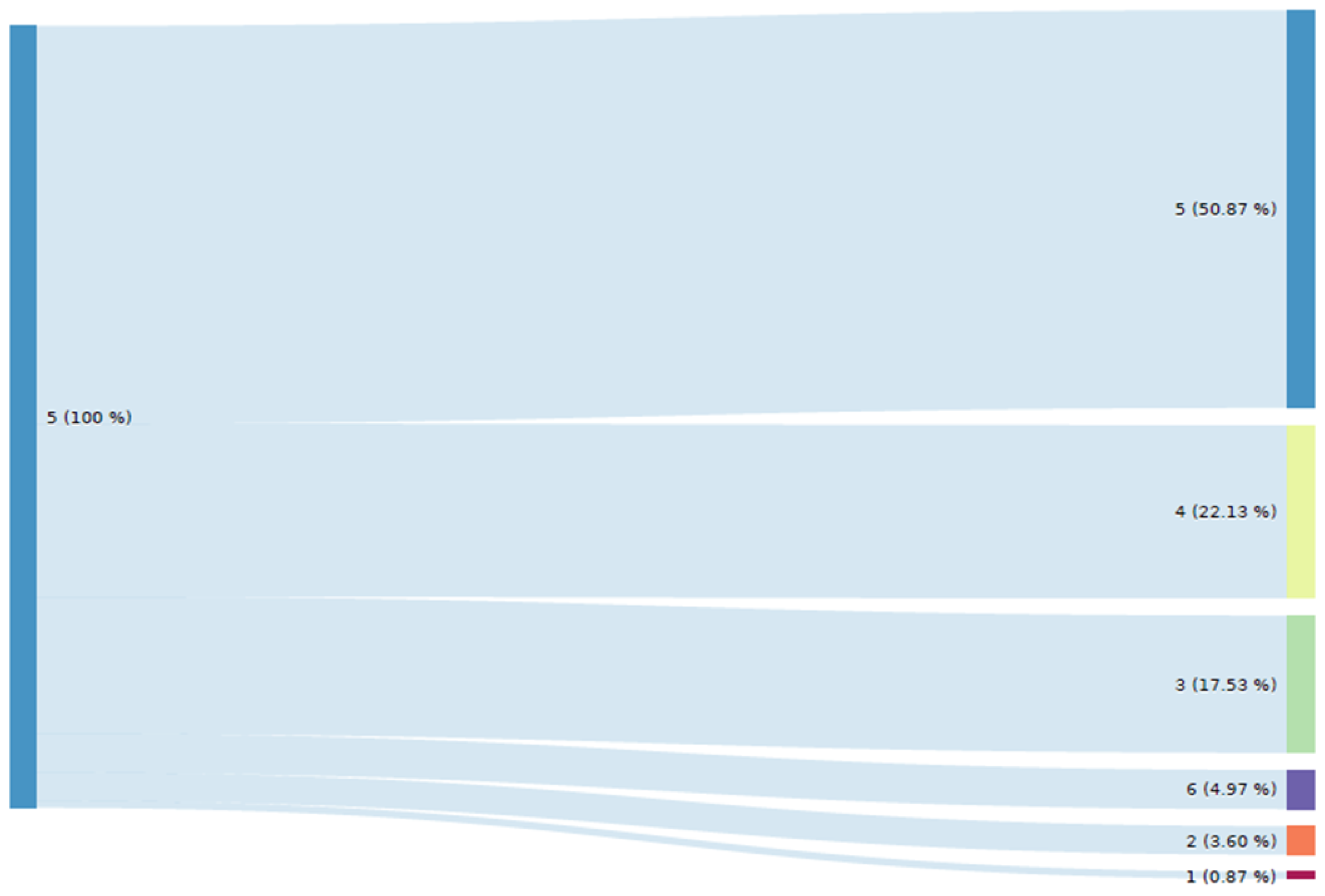
Figure 9 easier to interpret, only four months of each season are shown: January (Jan) for winter, April (Apr) for spring, July (Jul) for summer and October (Oct) for autumn. According to the results, the changing proportions in the clusters over the months of the year is due to consumers migrating from one cluster to another. This migration is explained by changes in consumer behavior that are strongly dependent on the temperature and on calendar events. For example, if we focus only on the migration of consumers in cluster 5 from January to April (see
Figure 10), we can see that
of the consumers move to clusters with lower levels of electricity consumption and a different profile (clusters 1, 2, 3 and 4); most of the changed consumers move to clusters 4 and 3, whose patterns are closely related to those of cluster 5, while the majority remain in cluster 5 (
), and only
migrate to a cluster with a higher electricity consumption level (cluster 6). To quantify the moving of consumers from one cluster to another, the global transition rates between clusters have been computed (see
Table 4). These rates have been computed from the clustering results (change in electricity consumption behavior over the months of 2010). As explained previously, it can be seen that for the majority of consumers, the probability of remaining in the same cluster is high (see the diagonal of
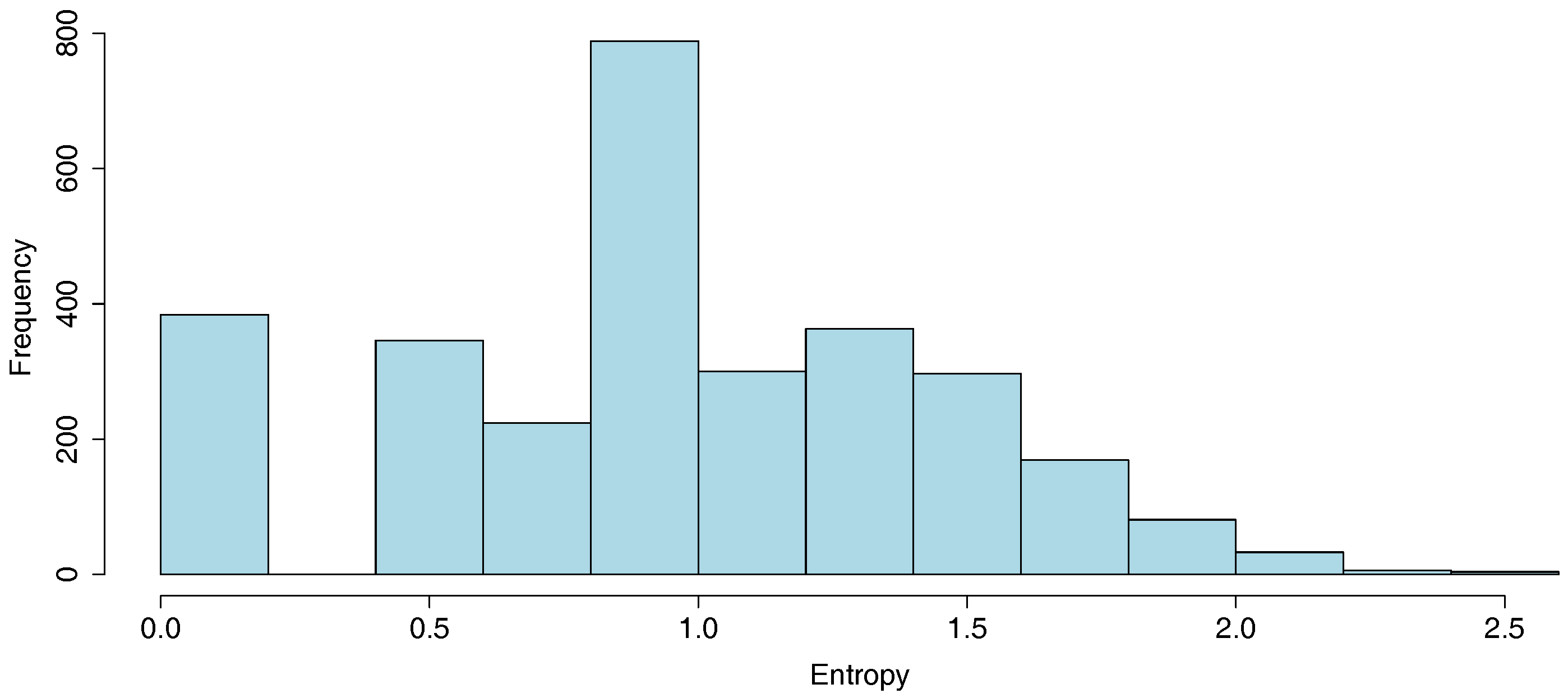
Table 4). Moving of consumers is generally detected between adjacent clusters. This depends on many reasons such as changes in the weather (“cold month to hot month” or “hot month to cold month”). The histogram that empirically describes the distribution of entropies
is displayed in
Figure 11. Three illustrations for low, medium and high entropies are also presented in
Figure 12. It can be seen that the entropy is close to 0 for consumers whose consumption behavior is regular. We also observe that the entropy of a large proportion of consumers is around 0.9. This part of the study may also help energy utilities to identify households that could be involved in a demand response process.
8. Conclusions
In this paper, a clustering approach was developed to identify typical electricity consumption profiles. The goal was to analyze the behaviors of Irish electricity consumers on the basis of electricity consumption data collected through smart meters. A generative model based on a specific Gaussian Mixture Model was designed. This model integrates a day type (Saturday, Sunday or weekday) as a time-dependent variable. Then, each cluster obtained is characterized by three profiles according to the day types. Six clusters were extracted from non-normalized residential data during the month of November, and an in-depth analysis was performed on the typical patterns. A similar study has also been conducted on the same data after normalization in order to investigate the impact of the standardization on the interpretation of consumers’ behavior. The residential behaviors depend mainly on the household’s socio-economic characteristics and on the times that the households are occupied during the day. The study showed that consumer behavior evolves over time depending on the temperature and on calendar events. The research detailed in this paper is useful for electricity utilities in developing new pricing policies, improving their load forecasting efficiency and identifying potential targets for demand-response service requests. A better understanding of the determinants of consumer behavior can also benefit urban modeling by providing simulation models with realistic and accurate energy consumption patterns. This detailed understanding is essential when thinking about the smart cities of the future.
The work presented in this paper represents a first step towards a more general framework based on generative models. Future work should take into account some additional considerations to extend this study. It would be interesting to incorporate a specific variable for holidays in the proposed generative model. One way of achieving this would be to use more precise calendar information. As one might expect, electricity consumption depends on many factors such as the day of the week (Monday, ..., Sunday), and the occurrence of a public holiday, a four-day weekend or a school holiday. This calendar information could be set manually or extracted by a preliminary clustering over the days of the year. In terms of modeling, this could easily be incorporated in the model by increasing the number of types of day encoded by the observed variable . However, in order to be effective, this kind of approach requires datasets that have been collected over longer periods (more than one year). In the same way, it would also be motivating to investigate on the integration of a seasonal encoding to the model. This enables to consider the periodic behavior of time series.
On the other hand, it would be challenging to investigate on energy consumption forecasting tools that use the same types of clustering results. Following the line of research in [
33,
34], we are currently engaged in work on this topic based on machine learning models such as non-homogeneous Markov models [
35] where forecasting uses the clustering results.


