Abstract
Research on graph comprehension suggests that point differences are easier to read in bar graphs, while trends are easier to read in line graphs. But are graph readers able to detect and use the most suited graph type for a given task? In this study, we applied a dual representation paradigm and eye tracking methodology to determine graph readers’ preferential processing of bar and line graphs while solving both point difference and trend tasks. Data were analyzed using linear mixed-effects models. Results show that participants shifted their graph preference depending on the task type and refined their preference over the course of the graph task. Implications for future research are discussed.
Introduction
Visualizations such as graphs and diagrams are ubiquitous in everyday human experience, and can be found in newspapers and television, as well as in science, engineering, and education (e.g., Blackwell, 2001; Glazer, 2011; Mayer, 2009; Pereira-Mendoza, Goh, & Bay, 2004; Purchase, 2014; Schnotz, 1994). They are especially important in the context of problem solving (Baker, Corbett & Koedinger, 2001), for teaching and learning mathematics (Cucuo & Curcio, 2001) and for understanding scientific data (Shah & Hoeffner, 2002).
To date, a large variety of different graph types have been developed (cf. Bertin, 1983; Kosslyn, 1989; Lohse, Biolsi, Walker, & Rueler, 1994). The advantages of graphs are computational because they support efficient computational processes (Larkin & Simon, 1987). Despite some similarities between the formats, computational differences between different graph types have been identified, even if two graphs are informationally equivalent (e.g., Kosslyn, 1989; Pinker, 1990). In general, two representations are called informationally equivalent when they display the same relations between the same objects, “because they are indistinguishable in terms of the information they represent” (Palmer, 1978, p. 270). Furthermore, two representations are called computationally equivalent when they are both informationally equivalent and “any inference that can be drawn easily and quickly from the information given explicitly in one can also be drawn easily and quickly from the information given explicitly in the other, and vice versa” (Larkin & Simon, 1987, p. 67).
A certain graph may facilitate information processing in some tasks, but not in others. For example, Simkin and Hastie (1987) used three informationally equivalent graph types and found that speed and accuracy in a graph task depended on the combination of graph type and task requirements. More recently, Peebles and Cheng (2003) discovered that the computational advantages of a graph may even compensate for a reader‘s unfamiliarity with a certain graph type as participants showed significant learning effects over time. These findings show that computational properties may affect one’s efficiency in completing graph tasks.
Yet, there is little knowledge about graph readers’ ability to detect and use computationally advantageous representations for a given task when given the choice. Accordingly, the main goal of the current study was to investigate graph readers’ ability to adapt their processing strategy to the demands of the task (i.e., preferring the graph type that is most suitable for solving a particular task). To accomplish this, we systematically varied the task type while presenting two informationally equivalent graphs that are known to be computationally different with regard to the tasks (see e.g., Pinker, 1990; Shah & Hoeffner, 2002). However, previous graph comprehension research using eye-tracking methodology has mainly focused on the processing of one graph at a time (e.g., Shah & Carpenter, 1995; Goldberg & Helfman, 2011; Kim & Lombardino, 2015; Peebles & Cheng, 2003). For the current study, we used a dual representation paradigm and eye-movement parameters to determine graph readers’ preferential usage of two graph types while processing a graph task.
Visual attention, measured by eye tracking, has repeatedly been used to establish a measure of preference, for example, in market research (e.g., Meissner & Decker, 2010), usability research (e.g., Djamasbi, Siegel, Skorinko, & Tullis, 2011) and in educational assessment with multiple-choice questions (Lindner et al., 2014). Building on this approach, we applied eye-movements as a measure of preference to the domain of graph comprehension.
In the following, we briefly review three important aspects of graph comprehension. First, we (1) introduce typical graph reading tasks, providing helpful insights into the nature of the graph tasks in the present study. Then we (2) outline the computational properties of different graph types. Finally, we (3) present findings on graph reading and learning effects.
Graph Reading Tasks
When it comes to graph reading tasks, a great number of taxonomies have been developed in the past decades, comprised of highly similar concepts (i.e., Bertin, 1983; Curcio, 1987; Schnotz, 1994; Tan & Benbasat, 1990; Wainer, 1992). Reviewing these classifications reveals a remarkable consensus across decades and authors that provides a high level of confidence that basic graph reading tasks can be identified with a high reliability. Tasks involving the recognition of relations between multiple elements are in the focus of the current study as they have been repeatedly classified as typical graph tasks. This includes identifying trends (e.g., a development in sales numbers over years) as well as identifying point differences (e.g., a difference in sales numbers between distinct years).
Computational Properties of Graphs
In graphs, information is not represented by a resemblance to physical objects. Instead, spatial relations between visual objects are employed as an analogy to nonspatial relations (e.g., Koerber, 2011; Winn, 1990). Often, inferences from non-spatial representations are relatively more demanding, because some information has to be computed at great cognitive costs (e.g., comparing numbers in a continuous text). Thus, graphs offer computational advantages in comparison to other forms of representations (Larkin & Simon, 1987).
Graphs are not only computationally different from other representations, such as text and tables, but also from each other (Schnotz, 2002; Wainer, 1992). A number of studies provide empirical support for the idea that differences in the computational characteristics of different graph types can explain task performance in typical graph tasks (e.g., Peebles & Cheng, 2003; Simkin & Hastie, 1987; Shah, Mayer, & Hegarty, 1999). In their review of graph comprehension literature, Shah and Hoeffner (2002) summarize that bar graphs emphasize point differences, while line graphs are more helpful for identifying trends. Taking a closer look at the processes that guide graph comprehension, Pinker (1990) outlines the computational differences between bar graphs and line graphs. He suggests that line graphs facilitate the observation of trends (trend task) because, in this format, a trend can correspond to a single visual attribute (e.g., slope) of a perceptual entity (line) in the display. In bar graphs, on the other hand, trends do not correspond to the attributes of single perceptual entities. Instead, the attributes (e.g., height) of multiple entities (bars) need to be kept in mind, which makes observing trends more effortful and error prone. An observation of point differences (difference task), on the other hand, can be made more easily using bar graphs, because bars are distinct entities and facilitate point estimates (Zacks & Tversky, 1999). For example, one might want to compare a company’s sales numbers for a set of particular years. Rather than looking at the numbers and computing the differences, viewers can use spatial analogies to make inferences about a non-spatial concept. In bar graphs, the horizontal position of the bars corresponds to a value on the depicted scale (e.g., years), and their height corresponds to a value on another scale (e.g., sales numbers). Using this graph type, readers can easily identify particular years because they are represented by distinct visual entities (bars). In a line graph, however, extracting distinct points is much more difficult because perceptual grouping (Wertheimer, 1938) causes each line to be encoded as a single entity rather than as a set of distinct points (Pinker, 1990). In summary, bar and line graphs are not computationally equivalent; rather, they provide very different computational advantages regarding trend and difference tasks. Thus, in combination, they seem useful in eliciting a shift in graph readers’ preferential processing.
Graph reading and learning effects
Basic graph reading skills can be observed as early as in preschool and middle school (e.g., Curcio, 1987; Koerber, 2011) and these skills develop over time (Lowrie & Diezmann, 2007). Nonetheless, unexperienced readers often make mistakes when interpreting graphs (Bell & Janvier, 1981; Shah & Carpenter, 1995; Shah & Hoeffner, 2002). Even among more experienced graph readers, task performance seems to vary (e.g., Ali & Peebles, 2013). As shown by Baker, Corbett and Koedinger (2001), graph readers’ misconceptions may arise from a lack of familiarity with some graph types. In contrast, a study with more experienced graph readers by Peebles and Cheng (2003) demonstrated a tradeoff between familiarity and the computational advantages of a given graph. The authors compared informationally equivalent graph types (a function line graph and a parametric line graph) and found that the effectiveness of a particular graph in retrieving the required information depended on the task, exposing computational differences between the formats. Even though participants were more familiar with one of the two graph types, they showed a significant learning effect after repeated exposure to the less familiar graph and were able to use it more effectively. These findings emphasize the importance of the computational properties inherent to different graph types as well as the potential of computational advantages to outweigh the cost of familiarization.
Looking at research on educational assessment, there is additional evidence that students are able to improve their performance over the course of a test due to learning effects regarding the handling of the given tasks (e.g., Hartig & Buchholz, 2012; Ren, Wang, Altmeyer, & Schweizer, 2014). Based on this, we assume that graph readers can improve their ability to adapt their processing strategy to the demands of a task, showing an increasing preference for the computationally advantageous graph over time.
Research Questions
According to a number of graph task classifications (Bertin, 1983; Curcio, 1987; Schnotz, 1994; Tan & Benbasat, 1990; Wainer, 1992), identifying trends and comparing point differences are regular tasks of graph reading that are often necessary for understanding and interpreting data sets. Furthermore, there is conclusive empirical evidence that task performance may be influenced by the graph type that is used to complete the task. For bar and line graphs, the computational advantages are very different: trends can be understood easier when reading line graphs instead of bar graphs, while the opposite is the case for understanding point differences. To date, there is little knowledge about graph readers’ ability to detect and use the graph most suited to a given task. Therefore, the aim of our study was to compare the processing of graphs in difference tasks and trend tasks, while presenting both line graphs and bar graphs at the same time.
Additionally, we investigated graph readers’ preference development as it unfolds across the experimental trials. Even though there is some evidence that graph readers may get more efficient in using the computational advantages of graphs over time (Peebles and Cheng, 2003), this second research question is comparatively novel and more explorative in nature.In summary, we expected the following:
(1) Preferential graph-processing hypothesis: Graph readers prefer the computationally advantageous graph type as a function of the task: (a) Graph readers prefer line graphs to bar graphs for tasks that require an observation of trends (trend tasks). (b) Graph readers prefer bar graphs to line graphs for tasks that require an observation of point differences (difference tasks).
(2) Preference development hypothesis: Over the course of processing multiple difference and the trend tasks, graph readers’ preference for the computationally advantageous graph type increases: (a) Graph readers’ preference for line graphs increases over the course of processing trend tasks. (b) Graph readers’ preference for bar graphs increases over the course of processing difference tasks.
Method
Sample and Study Design
The participants in our study were 32 students on the undergraduate level from different faculties (70% female, Mage = 24.37 years). All participants had normal or corrected to normal vision. Data from two participants (6 %) were excluded from the analysis due to the poor quality of the eye-tracking data, resulting in a final sample of N = 30 participants. The assessment comprised a set of graph tasks (difference and trend tasks) as well as a short paperpencil questionnaire to assess demographic information as well as participants’ graph literacy and overall preference for graph types as a control variable. For the graph tasks, we employed a within-subject design, in which we varied the task type (difference task vs. trend task) using different sets of true-false statements. In the difference task, participants had to evaluate the true-false statement by identifying point differences in the graphs (e.g., “In 2011, more new apartments were built than in 2013”). In the trend task, participants had to identify trends to complete an item (e.g., “Investments in climate protection have increased over the years”). There were 24 trials in each condition of the task type, resulting in a total of 48 trials per participant. Eye-movement data were recorded for each trial and each participant during processing of the graph tasks.
Material and Measures
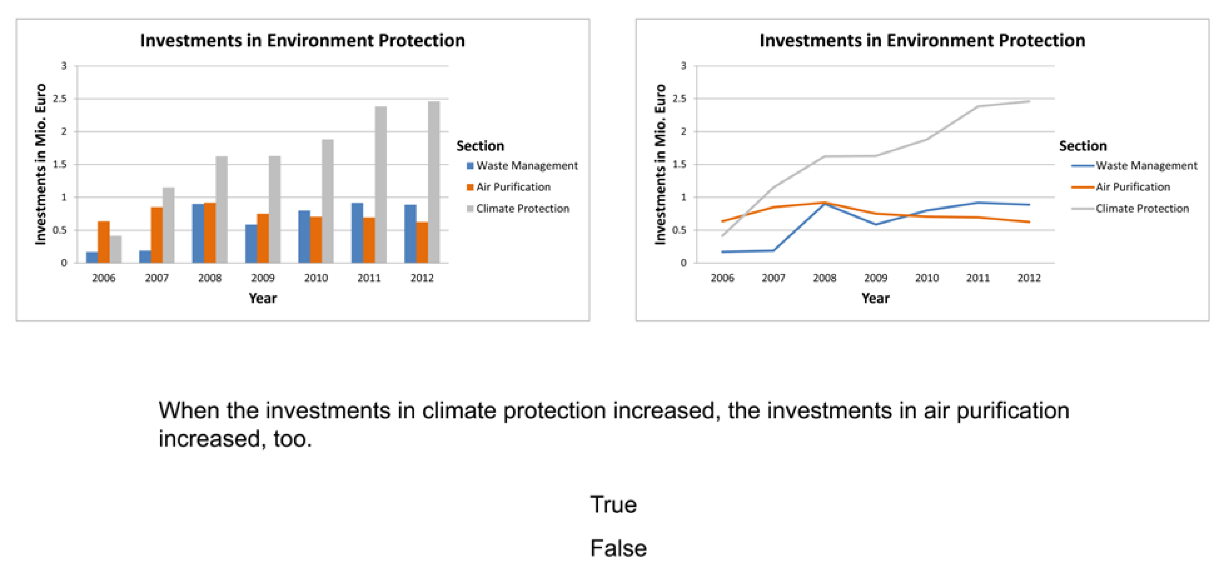
Graph Tasks. We developed a dual representation paradigm for an indirect preference measure using eyemovement data. Participants were confronted with two representations at the same time, followed by either a difference or trend task that could only be completed with information derived from the given graphs and did not require any previous knowledge. Each trial consisted of a pair of graphs, next to each other in the center of the display; one a bar graph, the other a line graph. Positions (left or right) of the two graph types were balanced randomized. A statement was displayed below the pair of graphs, followed by the choices “true” and “false”, which could be selected by participants as a response with a mouse click. True-false items are known to function differently depending on whether they are true or false (Grosse & Wright, 1985; for a detailed overview see Haladyna, 2004), so we balanced the number of true and false statements throughout the test. Both graphs of each pair were constructed using the same data set, resulting in two informationally equivalent graphs. Data sets were taken from the Federal Statistical Office in Germany, using the office’s website (www.destatis.de). By using real data sets, we reduced the risk of disbelief resulting from an implausibility of the data. Data were refined to achieve comparable complexity throughout all items. Each pair of graphs displayed three variables employing the x-axis, y-axis and legend of the graphs. Data points were trimmed to show between five and eight occurrences on the x- and y-axis and three categories conveyed by differing colors. Identical labels and legends were used in both graph types. A translated example is given in Figure 1.

Figure 1.
Sample stimulus of the graph tasks (translated from German).
Paper-Pencil Questionnaire. A short questionnaire was employed to survey participants’ graph literacy and overall preference for the two graph types (bar graph vs. line graph) using a 5-point Likert scale. The graph literacy scale was comprised of two items (i.e., “I am good at reading graphs”, “I feel confident in reading graphs.”). Another two items were used to assess the overall preference. Here, one item was the inverse of the other (“Generally, I prefer bar graphs to line graphs” and “Generally I prefer line graphs to bar graphs”). To facilitate interpretation, the overall graph preference was calculated as the difference between the preference scores of the two items. Positive values indicate an overall preference for bar graphs, whereas negative values indicate an overall preference for line graphs.
Apparatus
Items were presented on a 19-inch screen with a 1280 × 1024 pixel resolution, using the software Experiment Center 3.4 from SensoMotoric Instruments (SMI, Teltow, Germany). Each item was presented on a single screen. While working on the test, participants sat in front of the screen at a distance of approximately 70 centimeters. The font size of the text was 2 centimeters (approx. 1.6° visual angle). Both graphs had an identical total size of 17.7 × 9.9 centimeters (approx. 14.4° visual angle in width and 8.1° visual angle in height) and were displayed next to each other with a gap of 0.8 centimeters (approximately 0.7° visual angle) in the center of the screen. Participants’ eye-movements were recorded using a video-based remote eye-tracking system (SMI iView X™RED-m; 120Hz sampling rate) and the corresponding SMI software iView X™. The system was calibrated using an animated 8-point calibration image and subsequent validation. The calibration accuracy was below 0.49° of the visual angle for all participants on both the x and y coordinates (range: 0.09 to 0.48; Mx = 0.32, SDx = 0.08; My = 0.29, SDy = 0.11).
Procedure
Students were tested in single sessions. First, they were familiarized with the procedure and the eye-tracking system; after this, they completed the graph tasks on a computer while their eye-movements were recorded. Participants were informed that both graphs in each item conveyed the same information. However, they received no particular instructions on how to choose between the given representations. Participants could therefore employ a solution strategy based on their individual preference instead of following a strategy that was either given or implied. The paper-pencil questionnaire was administered after participants completed the graph task. The whole cycle of assessment took about 30 minutes to complete.
Analysis
Eye-Movement Data Pre-Processing. Eye-movement recordings were analyzed using a dispersion-based algorithm implemented in the Begaze™ software, version 3.5, from SMI. A fixation was detected when eye movements lasted for at least 80 milliseconds on a position with a maximum dispersion of 100 pixels. To determine whether eye-movement data were recorded correctly, participants’ scan paths were visually inspected using Begaze™ software, version 3.5, from SMI.
As gaze data, we used the total fixation time on predefined Areas of Interest (AoIs), which is defined as the cumulative duration of all AoI fixations from trial onset to task end, indicating the total time devoted to a specific area (Holmqvist et al., 2011). Relying on the eye-mind hypothesis (Just & Carpenter, 1980), we assume that points of fixation represent the focus of attention, so that eye movements reflect the spatiotemporal encoding of visual information. Fixation times provide a valid indirect measure of attention distribution and cognitive processing in educational tasks, such as solving test items in a multiple-choice format (see e.g., Lindner et al., 2014).
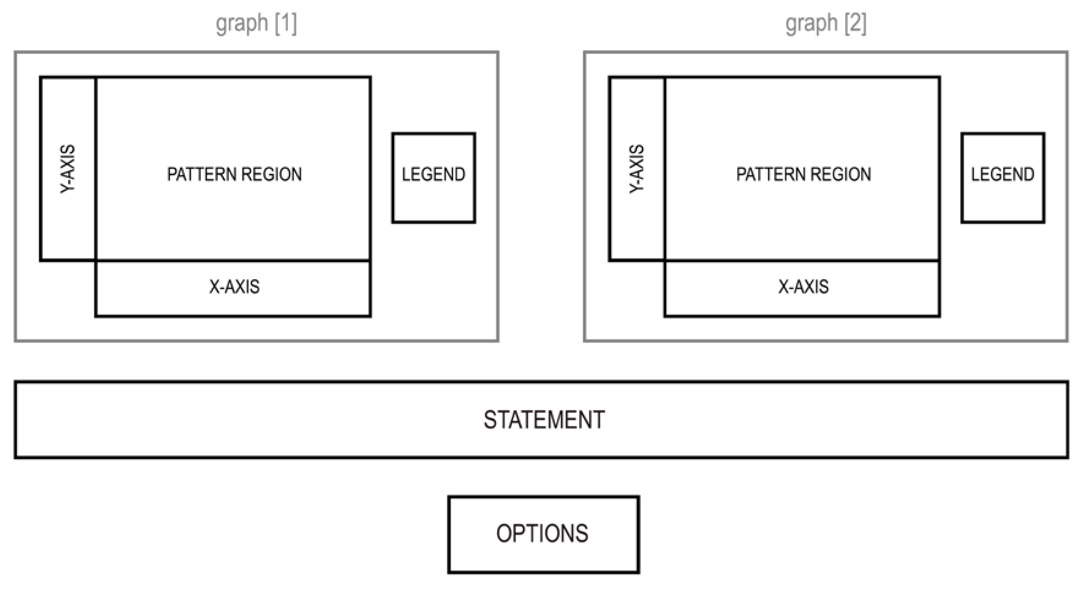
As in previous graph studies (e.g., Carpenter & Shah, 1995; Kim & Lombardino, 2015; Peebles & Cheng, 2003), we divided the graph regions into four rectangular AoIs: x-axis, y-axis, legend, and pattern, defined separately for each of the two graphs, in addition to the statement and option (true/false) regions, resulting in a total of ten AoIs (Figure 2). The AoIs covering the pattern regions were about the same size in every display and for the two graph types within a display (approx. 10 x 7 cm). Because the graph reading processes necessary to complete the tasks occur within the pattern area of the graph (e.g., comparing heights of bars or slopes of lines), we compared fixation times on the pattern regions.
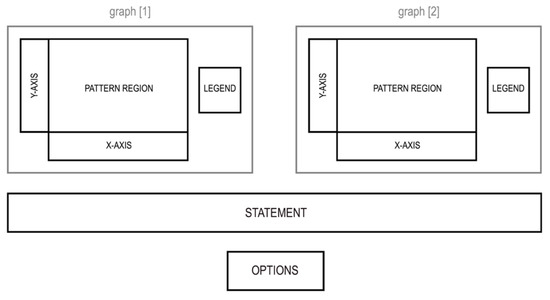
Figure 2.
Composition of Areas of Interest (in capital letters) defined for the eye-tracking analysis.
Preferential processing of one graph over the other graph was defined as the difference between total fixation times on the pattern regions of the two graphs. However, not all fixations during a trial reflect preference. In order to decide which graph to use for task completion, participants must first read the statement to identify the task type. Accordingly, only fixations that occurred after the first fixation of the statement region were used to compute the preference measure.
Linear mixed-effects models. All data were analyzed using R, version 3.1.0 for Windows (R Development Core Team, 2015). With repeated measures nested within participants as well as in items, the data structure can be described as clustered or hierarchical (Snijders & Bosker, 2012). Since the repeated measures were nested within two higher-level units, the test design is called crossclassified ((i.e., each measure belongs uniquely to one participant and one item; Snijders & Bosker, 2012). Regular approaches, such as ANOVA models, yield inflated Type I error rates when the data is clustered (Dorman, 2008). To account for the clustered data structure, we applied linear mixed-effects models (LMMs; for introductions, see Barr, 2008; Snijders & Bosker, 2012; Quené & van den Bergh, 2008). These models can be conceptualized “as a series of interrelated regression models that explain sources of variance at multiple levels of analysis, such as at the experimental stimuli and person levels” (Hoffman & Rovine, 2007, p. 102). More specific, LMMs can model fixed effects and random effects simultaneously. While fixed effects aim to identify the typical rates of change in the outcome variable (e.g., following an experimental manipulation), random effects aim to identify unsystematic rates of change (e.g., due to differences between items and persons, respectively).
We used the R package lme4 (Bates, Maechler & Bolker, 2015) to perform a linear mixed-effects analysis of the relationship between the relative graph preference and several explanatory variables in four models: First, we computed an empty model with random intercepts for subjects and stimuli (M0) in order to gain insights into the variance structure of the data. To test our hypotheses, we included fixed effects for task type, trial number, and the task type by trial number interaction (M1). Then, we added the participants’ overall graph preference as a control variable for individual preferences (M2). Finally, we added random effects by including by-subject random slopes for the effects of task type and trial number to account for differences in individual trajectories between tasks and over time (Barr, Levy, Scheepers & Tily, 2013; M3). Models were fitted by the Restricted Maximum Likelihood (REML) criterion since it yields better Type I error rates for smaller groups (N ≤ 50) when testing fixed effects than estimates with the Maximum Likelihood (ML) criterion (Manor and Zucker, 2004; Snijders & Bosker, 2012).
Results
The ratings of graph literacy in the current sample were relatively high (M = 3.55, SD = 0.83, range = 2 to 5), with the graph literacy scale showing a good reliability (Cronbach’s α = .82). Participants achieved a correspondingly high average accuracy in the graph tasks, 89% in the trend task and 90 % in the difference task. There was no significant difference in participants’ performance between the task types (t29 = 0.61, p = .55). Because gaze data may differ for correct and incorrect responses, we removed data of incorrect responses from our analyses.
Average total fixation times and average percentages of processing time on the predefined AoIs across items and participants in the two task conditions are given in Table 1. Data showed a noticeable difference in total processing time between the two graph tasks. We compared the average total processing time across participants for trials in the difference task versus trials in the trend task using a paired t-test in order to confirm that this difference was significant (t23 = 4.53, p < .001, d = 0.92). This is also reflected by a significant difference in total fixation time on the statement area (t23 = 5.90, p < .001, d = 1.20). To account for this bias in processing time, we computed the total relative fixation time (percentage of processing time) for each trial of each participant as the total fixation time (on AoIs) relative to the total processing time of the respective trial. As the preference measure, we computed the relative graph preference as the difference between total relative fixation time on the bar graph pattern region and total relative fixation time on the line graph pattern region in percentage points. Difference values were calculated for each trial from each participant. Positive values indicate preferential processing of the bar graph, whereas negative values indicate a preference for the line graph.

Table 1.
Average total fixation times (in ms) and average percentages of processing time (in %) on predefined Areas of Interest for difference and trend task conditions across items (24 trials per condition) and participants (n=30).
Regarding the linear mixed-effects models, a visual inspection of residual plots did not reveal obvious deviations from homoscedasticity or normality. Table 2 shows the fixed effects and variance components of the random effects in the linear mixed-effects models described above. Analyzing the empty model (M0), the intraclass correlations (ICC) for subjects and stimuli revealed that substantial portions of variance can be attributed to differences between subjects and stimuli, respectively (ICCSubject = 0.11; ICCStimulus = 0.19). To perform likelihood ratio tests (LRT), each model was refitted using ML instead of REML because the LRT for fixed effects using REML is known to be inappropriate (Pinheiro & Bates, 2000; Snijders & Bosker, 2012). LRTs showed that each addition of explanatory variables (as described above) was a significant contribution to the model (see Table 2) (In addition, we included interaction terms in the fixed effects for overall graph preference, but the change in deviance was nonsignificant (χ2[3] = 1.53, p = .68). Thus, this model was omitted.). Regression lines of the fixed effects in M3 are given in Figure 3. The following sections focus on the fixed effects in Model M3 in order to address our research questions.
Table 2.
Comparison of fixed effects and random effects in the linear mixed-effects models.

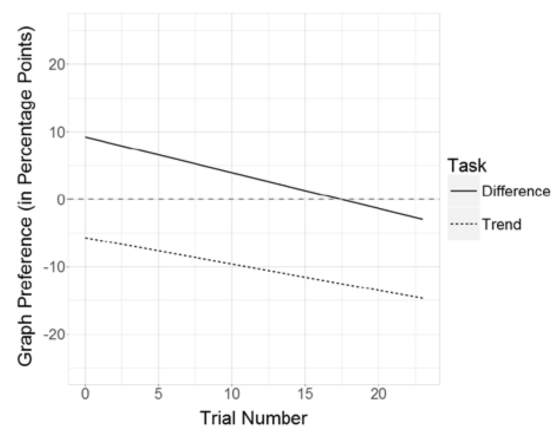
Figure 3.
Regression lines of the fixed effects in Model 3, given a neutral (= 0) overall graph preference.
Overall Graph Preference
Even though participants varied in their overall graph preference, there was no global bias towards one of the two graph types (M = 0.34; SD = 1.70; Range = -3 to 3).
To control for individual preferences for one of the graph types, we included participants’ reported graph preference in the linear mixed-effects models. Comparing models M1 and M2, the inclusion of this variable explained a small portion of the subject-related variance in the random part of the model. The change in deviance between the two models was significant (χ2[1] = 5.30; p < .05). In the final LMM (M3), the overall graph preference showed a significant positive relation to the relative graph preference (p < .05). A change of one point in the overall graph preference score resulted, on average, in a change of 1.4 percentage points in the same direction in the estimated relative graph preference. This means that participants who reported a preference for one of the graph types also showed a slightly higher preference for that graph type during item processing.
Preferential Graph Processing
First, we hypothesized that participants would prefer line graphs to bar graphs in trend tasks (Hypothesis 1a), whereas a preference of bar graphs was expected in difference tasks (Hypothesis 1b). Analyzing the fixed effects in the final LMM (M3), task type had a substantial impact on the relative graph preference: A change in task type from difference task to trend task lowered the estimated relative graph preference by about 15 percentage points. This difference was significant (p < .001; Table 2). For participants with no reported preference for either graph type, this change indicates, on average, a preference shift from bar graphs in difference tasks to line graphs in trend tasks. For example, in the first trial of the difference task, participants had, on average, a relative preference of 9 percentage points in favor of bar graphs. In the first trial of the trend task, however, participants showed a relative preference of 6 percentage points in favor of line graphs. In addition to the linear mixed- effects models, we conducted two paired t-tests in order to compare relative fixation times on bar graphs versus line graphs separately for each task condition. Here, total relative fixation times on bar graphs and on line graphs were aggregated across items for each participant. In the trend task, participants devoted significantly less time to the processing of the bar graph compared to the line graph (t29 = -4.97, p < .001, d = 0.91) and vice versa in the difference task (t29 = 2.75, p < .05, d = 0.50), with the effect size in the trend task being almost twice the size of that in the difference task. Both the results from the linear mixed-effects model and the additional t-tests are in line with our preferential graph-processing hypotheses (1a, 1b).
Preference Development
Second, we expected participants to develop a stronger preference for line graphs in the trend task over time (Hypothesis 2a), whereas we expected participants to develop a stronger preference for bar graphs in the difference task (Hypothesis 2b). The LMM (M3) revealed a significant fixed effect of trial number (p < .05; Table 2), whereas the fixed effect of the trial number by task type interaction was not significant (p = .52; Table 2). From one trial to the next, on average, the estimated relative preference was reduced by about 0.5 percentage points in the difference task and by about 0.4 percentage points in the trend task, indicating that participants developed a stronger preference for line graphs both in the trend and in the difference task. However, for the difference task, we had predicted a change in the opposite direction. These findings are in line with hypothesis 2a, but could not confirm hypothesis 2b. Possible explanations for this finding are discussed below.
Discussion
In this study, we investigated the relationship between graph readers’ preferential processing of bar versus line graphs when solving both difference tasks and trend tasks. Theoretical approaches and empirical studies suggest that bar graphs have computational advantages for difference tasks, whereas line graphs are advantageous for trend tasks, facilitating the task-directed processing of the depicted data (e.g., Pinker, 1990; Shah & Hoeffner, 2002). We investigated (1) participants’ relative graph preference for bar versus line graphs, and (2) the preference development across time, in order to determine whether graph readers are able to detect and use the advantageous graph type when solving difference and trend tasks. In an experimental setting, we employed a dual representation paradigm (i.e., displaying two graph types at the same time) and eye-tracking measures to determine the preferential processing of bar versus line graphs.
Our results show that the graph readers in our sample of university students had, on average, a stronger preference for using bar graphs than for using line graphs in difference tasks and vice versa in trend tasks, indicating that they had a tendency to choose the computationally advantageous graph type as a function of the task. However, we also found an increase in the preference for line graphs in both task conditions, resulting in a strong preferential processing of line graphs in trend tasks and a balanced use of both graph types in difference tasks.
Overall Graph Preference
To control for individual differences in preference beyond the experimental manipulation, we asked for participants’ overall preference for bar graphs versus line graphs. The inclusion of this covariate into the LMM revealed a positive relation to the relative graph preference, which provides tentative evidence that the eyemovement-based measure of preference was a valid indicator of participants’ actual graph preference. Additionally, it supports the conclusion by Shah (2002) that graph comprehension is a product of both bottom-up and topdown processes, which seem to consist not only of expectations and familiarity with content, but also of an individual preference for a certain type of representation (i.e., the graph type). However, the fixed effect of the overall graph preference was relatively small compared to the fixed effect of the task type (Table 2). In accordance with this, the context (e.g., the task type) in which a graph is presented seems to be far more predictive of graph readers’ processing behavior than a judgment of their overall graph preference.
Preferential Graph Processing
The results from our final LMM (M3) show that participants shifted their preference from bar graphs in difference tasks to line graphs in trend tasks. Additional t- tests using aggregated data revealed that the difference in total fixation times on the two graphs was significant in both task conditions. However, the effect size was approximately twice as large in the trend task, suggesting that participants had an even stronger tendency towards the advantageous graph type when processing trend tasks. One explanation for this finding might be that the computational advantages of line graphs in trend tasks are stronger than those of bar graphs in difference tasks, due to working-memory limitations: When solving trend task items using bar graphs, participants always had to consider all five to eight data points at once to constitute a trend (Pinker, 1990), thereby operating at the limits of working memory (Baddeley, 1994; Baddeley & Hitch, 1972; Miller, 1956). On the other hand, when solving trend task items using line graphs, they only needed to inspect a single line, which puts relatively small demands on working memory, in comparison to the demands placed by bar graphs. This difference in cognitive demands might explain the larger effect size in the trend task.
Looking at the difference task, even though comparing data points on a single line may be more difficult according to the Gestalt laws of perceptual grouping (Pinker, 1990) finding the correct positions among only five to eight data points may not have been too difficult. However, the true-false statements used in difference tasks may be responsible for the smaller effect size in this condition. Before examining the graphs, participants need to read the statement and keep in mind the relation that is described. While statements in the trend task only refer to single categories, those in the difference task explicitly mention multiple specific data points that must be compared. Thus, engaging with the statement in the difference task may be more difficult and demanding than in the trend task. This assumption is supported by the finding that participants spent significantly more time on the statement area when processing difference tasks. In the framework of Cognitive Load Theory (Sweller, 1988), it is assumed that cognitive processing is constrained by a limited working memory capacity and that the inherent characteristics of a task may put a higher demand on cognitive processes (intrinsic cognitive load; De Jong, 2010). Based on this, it seems possible that statements of the difference task put a greater cognitive load on participants. Since participants’ cognitive resources were burdened with keeping multiple data points in mind before even tending to the graph itself, their ability to choose the advantageous graph type in difference tasks may have been impaired. However, there might be another explanation: Participants unsystematically reported that they sometimes used both graph types to double-check their answer. This is a strategy that has been reported in earlier research. Peebles and Cheng (2003) argued that such a strategy helped graph readers to memorize the chunk of information previously viewed. In the dual representation paradigm, participants may have expanded this strategy to repeatedly revisit the same regions in both graphs. A post-hoc analysis of gaze transitions between the statement area and the graph pattern areas revealed a significantly higher average number of gaze transitions in trials of the difference task compared to trials of the trend task (MDifference = 4.05, MTrend = 2.11, t23 = 7.94 p < .001, d = 1.62), supporting this assumption. In summary, the statements in the difference task seemed to be more demanding, causing participants to verify their answer by checking both graph types repeatedly.
Preference Development
We hypothesized that participants would develop a stronger preference for bar graphs when solving difference task items and a stronger preference for line graphs when solving trend task items. To investigate this, we compared participants’ relative graph preference across the experimental trials. The results of the LMM (M3) suggest that participants developed a stronger preference for line graphs in both task conditions, confirming only one of our hypotheses (2b: preference for bar graphs increases over the course of processing difference tasks.), but not the other (2a: preference for line graphs increases over the course of processing trend tasks).
While the described development was expected in the trend task, it was a counterintuitive observation in the difference task. As there was no significant trial by task type interaction, the fixed effect of the trial number was very similar in both task conditions. Yet, the meaning of this development seems to be different for the two task types: In the trend task, on average participants started with a negative relative graph preference (i.e., preference for line graphs) that became stronger over time (this in line with our hypothesis 2b). In the difference task, on the other hand, participants started, on average, with a positive relative graph preference (i.e., preference for bar graphs) that decreased over time and became about zero (i.e., no preference for a particular graph, meaning fixation times on bar and line graphs were about equal). While this is contrary to our hypothesis 2a, it does not reflect a complete shift in preference, but rather a balanced use of both graph types when processing difference tasks. There might be more than one explanation for this finding: First, participants increasingly tended to use both graph types in the difference task, because verifying the answer proved helpful to evaluate the statements. However, because of the participants’ generally high accuracy, it remains unclear if this strategy was actually advantageous. Or second, participants generally developed a higher preference for line graphs over the course of the trials. This might be due to a transfer effect (for transfer effects in graph tasks see Baker, Corbett & Koedinger, 2001) from the trend tasks in which line graphs were more clearly advantageous as suggested by the higher effect size in this condition.
Conclusions
Computational properties of graphs have been investigated extensively in the past (e.g., Peebles & Cheng, 2003; Pinker, 1990; Simkin & Hastie, 1987; Shah, Mayer, & Hegarty, 1999; Zacks & Tversky, 1999). It is well established that line graphs are advantageous for trend tasks, while bar graphs are more helpful for difference tasks. However, there is little knowledge about graph readers’ ability to detect and use these properties. The current study contributes to the field of graph comprehension by investigating graph readers’ ability to choose the graph type most suited to a given task. Eye-tracking methodology was applied to assess graph readers’ preferential processing of bar versus line graphs in a dual representation paradigm. Data showed that computational advantages of bar and line graphs were reflected by participants’ preference towards the advantageous graph as a function of the task. Graph readers preferred to use the graph type most suited to a given task, suggesting that computational advantages in graphs are readily available to graph users, even in environments that provide alternative representations.
Still, there are limitations to our study that need to be considered.
First, the true-false items used in the graph tasks were not designed to be sensitive to differences in graph readers’ task performance and thus caused a ceiling effect in the performance data. Therefore, it remains unclear whether the observed preference patterns actually resulted in higher performance. Future studies could employ more complex tasks to investigate the connection between preferential processing and task performance.
Second, it is important to note that we used self-report data to assess participants’ overall graph preference. Since it was not possible to verify the validity of participants’ self-reports, this data should be interpreted with caution.
Third, we discovered that the true-false statements used in the difference task were relatively more demanding than those used in the trend task, which seems to have led participants to use both graphs in order to verify their answer. Additional research is needed to clarify the use of verifying strategies when multiple representations are available, for example, by complementing eye-tracking analyses with verbal reports (Ericsson & Simon, 1980; van Gog, Kester, Nievelstein, Giesbers, & Paas, 2009).
Fourth, we only investigated two different task types to analyze the preferential processing of bar graphs versus line graphs. Future studies could expand this research to additional tasks (especially more complex tasks) and more graph types (e.g., circle charts).
Finally, the number of participants in the current study was relatively small. However, by using a high number of experimental trials and employing linear mixed-effects models to account for the clustered data structure, we were able to compensate for this shortcoming. Still, future studies could collect data from larger samples to increase the reliability and generalizability of the results.
The findings and limitations of this study lead to some suggestions for future research. An analysis across trials revealed a general increase in the preference for line graphs, resulting in a strong preference for line graphs in trend tasks and a balanced use of both graph types in difference tasks. This unexpected preference development towards line graphs in both graph tasks poses new questions: Is the use of two graphs superior to using only one graph? May the graph preference be influenced by transfer effects between different tasks? Future research should investigate processing of multiple graphs compared to single representations to clarify if the use of multiple graphs can be advantageous for some tasks. Alternative explanations, such as transfer effects between multiple tasks, could also be investigated.
Furthermore, it should be noted that the random effects in the LMMs showed a substantial variation in the observed graph preference between participants, emphasizing the need to further explore individual differences in the domain of graph comprehension. Additionally, high processing times in the difference task revealed that these items may put a higher demand on working memory. Even though working memory has been discussed as a limiting factor for graph comprehension (e.g., Lohse, 1997; Pinker, 1990; Shah & Hoeffner, 2002; Trickett & Trafton, 2006), it has rarely been focused on. Only recently, Halford, Baker, McCredden and Bain (2005) found that the human processing capacity is limited to four variables in one graphical display. Thus, future research should consider individual variables, such as working memory capacity, alongside processing and performance data. A combination of these approaches could provide a deeper insight into graph readers’ ability to make use of computational properties, and into graph comprehension in general.
Acknowledgments
We thank Simon Grund for his valuable support with the linear mixed-effects analyses.
References
- Ali, N., and D. Peebles. 2013. The effect of gestalt laws of perceptual organization on the comprehension of three-variable bar and line graphs. Human Factors: The Journal of the Human Factors and Ergonomics Society 55, 1: 183–203. [Google Scholar] [CrossRef] [PubMed]
- Baddeley, A. D. 1994. The magical number seven: Still magic after all these years? Psychological Review 101: 353–356. [Google Scholar] [CrossRef] [PubMed]
- Baddeley, A. D., and G. Hitch. 1974. Working Memory. Psychology of Learning and Motivation 8: 47–89. [Google Scholar] [CrossRef]
- Baker, R. S., A. T. Corbett, and K. R. Koedinger. 2001. Toward a model of learning data representations. Edited by J. D. Moore and K. Stenning. In Proceedings of the Twenty-Third Annual Conference of the Cognitive Science Society. Mahwah, NJ: Erlbaum: pp. 45–50. [Google Scholar]
- Barr, D. J. 2008. Analyzing ‘visual world’ eyetracking data using multilevel logistic regression. Journal of Memory and Language 59: 457–474. [Google Scholar] [CrossRef]
- Barr, D. J., R. Levy, C. Scheepers, and H. J. Tily. 2013. Random effects structure for confirmatory hypothesis testing: Keep it maximal. Journal of Memory and Language 68: 255–278. [Google Scholar] [CrossRef]
- Bates, D., M. Maechler, B. Bolker, and S. Walker. 2015. Fitting Linear Mixed-Effects Models Using lme4. Journal of Statistical Software 67: 1–48. [Google Scholar] [CrossRef]
- Bell, A., and C. Janvier. 1981. The Interpretation of Graphs Representing Situations. For the Learning of Mathematics 2: 34–42, Retrieved from http://eric.ed.gov/?id=EJ255422. [Google Scholar]
- Bertin, J. 1983. Semiology of graphics: Diagrams, networks, maps. Madison, WI: University of Wisconsin Press. [Google Scholar]
- Blackwell, A. F. 2001. Introduction Thinking with Diagrams. In Thinking with Diagrams. Netherlands: Springer: pp. 1–3. [Google Scholar]
- Cucuo, A. A., and F. Curcio. 2001. The role of representation in school mathematics: National Council of Teachers of Mathematics Yearbook. Reston, VA: NCTM. [Google Scholar]
- Curcio, F. R. 1987. Comprehension of mathematical relationships expressed in graphs. Journal for Research in Mathematics Education 18: 382–393. [Google Scholar] [CrossRef]
- De Jong, T. 2010. Cognitive load theory, educational research, and instructional design: Some food for thought. Instructional Science 38: 105–134. [Google Scholar] [CrossRef]
- Djamasbi, S., M. Siegel, J. Skorinko, and T. Tullis. 2011. Online viewing and aesthetic preferences of generation y and the baby boom generation: Testing user web site experience through eye tracking. International Journal of Electronic Commerce 15, 4: 121–158. [Google Scholar] [CrossRef]
- Dorman, J. P. 2008. The effect of clustering on statistical tests: An illustration using classroom environment data. Educational Psychology 28: 583–595. [Google Scholar] [CrossRef]
- Ericsson, K. A., and H. A. Simon. 1980. Verbal reports as data. Psychological Review 87: 215–251. [Google Scholar] [CrossRef]
- Glazer, N. 2011. Challenges with graph interpretation: A review of the literature. Studies in Science Education 47: 183–210. [Google Scholar] [CrossRef]
- Goldberg, J., and J. Helfman. 2011. Eye tracking for visualization evaluation: Reading values on linear versus radial graphs. Information Visualization 10: 182–195. [Google Scholar] [CrossRef]
- Grosse, M. E., and B. D. Wright. 1985. Validity and reliability of true-false tests. Educational and Psychological Measurement 45: 1–13. [Google Scholar] [CrossRef]
- Haladyna, T. M. 2004. Developing and validating multiple-choice test items. New York, NY: Routledge. [Google Scholar]
- Halford, G. S., R. Baker, J. E. McCredden, and J. D. Bain. 2005. How many variables can humans process? Psychological Science 16: 70–76. [Google Scholar] [CrossRef]
- Hartig, J., and J. Buchholz. 2012. A multilevel item response model for item position effects and individual persistence. Psychological Test and Assessment Modeling 54: 418–431. [Google Scholar]
- Hoffman, L., and M. J. Rovine. 2007. Multilevel models for the experimental psychologist: Foundations and illustrative examples. Behavior Research Methods 39: 101–117. [Google Scholar] [CrossRef]
- Holmqvist, K., M. Nyström, R. Andersson, R. Dewhurst, H. Jarodzka, and J. De Weijer. 2011. Eye tracking: A comprehensive guide to methods and measures. Oxford, UK: Oxford University Press. [Google Scholar]
- Just, M. A., and P. A. Carpenter. 1980. A theory of reading: From eye fixations to comprehension. Psychological Review 87: 329–354. [Google Scholar] [CrossRef]
- Kim, S., and L. Lombardino. 2015. Comparing graphs and text: Effects of complexity and task. Journal of Eye Movement Research 8, 3: 1–17. [Google Scholar] [CrossRef]
- Koerber, S. 2011. Der Umgang mit visuell-grafischen Repräsentationen im Grundschulalter. Unterrichtswissenschaft 39: 49–62. [Google Scholar] [CrossRef]
- Kosslyn, S. M. 1989. Understanding charts and graphs. Applied Cognitive Psychology 3: 185–225. [Google Scholar] [CrossRef]
- Larkin, J. H., and H. A. Simon. 1987. Why a diagram is (sometimes) worth ten thousand words. Cognitive Science 11: 65–100. [Google Scholar] [CrossRef]
- Lohse, G. L., K. Biolsi, N. Walker, and H. H. Rueter. 1994. A classification of visual representations. Communications of the ACM, vol. 37, pp. 36–49. [Google Scholar] [CrossRef]
- Lindner, M. A., A. Eitel, G.-B. Thoma, I. M. Dalehefte, J. M. Ihme, and O. Köller. 2014. Tracking the decision making process in multiple-choice assessment: Evidence from eye movements. Applied Cognitive Psychology 28: 738–752. [Google Scholar] [CrossRef]
- Lowrie, T., and C. M. Diezmann. 2007. Solving graphics problems: Student performance in junior grades. The Journal of Educational Research 100: 369–378. [Google Scholar] [CrossRef]
- Mayer, R. E. 2009. Multimedia learning, 2nd ed. New York, NY: Cambridge University Press. [Google Scholar] [CrossRef]
- Meissner, M., and R. Decker. 2010. Eye-tracking information processing in choice-based conjoint analysis. International Journal of Market Research 52: 591–610. [Google Scholar] [CrossRef]
- Miller, G. A. 1956. The magical number seven, plus or minus two: Some limits on our capacity for processing information. Psychological Review 101: 343–352. [Google Scholar] [CrossRef]
- Palmer, S. E. 1978. Fundamental aspects of cognitive representation. Edited by E. Rosch and B. B. Lloyd. In Cognition and categorization. Hillsdale, NJ: Lawrence Erlbaum: pp. 259–303. [Google Scholar]
- Peebles, D., and P. C. H. Cheng. 2003. Modeling the effect of task and graphical representation on response latency in a graph reading task. Human Factors: The Journal of the Human Factors and Ergonomics Society 45: 28–46. [Google Scholar] [CrossRef]
- Pereira-Mendoza, L., S. L. Goh, and W. Bay. 2004. Interpreting graphs from newspapers: Evidence of going beyond the data. Paper presented at the ERAS Conference, Singapore, November; Available online: https://repository.nie.edu.sg/bitstream/10497/15549/1/ ERAS-2004-277_a.pdf.
- Pinheiro, J., and D. Bates. 2006. Mixed-effects models in S and S-PLUS. New York: Springer. [Google Scholar]
- Pinker, S. 1990. A theory of graph comprehension. Edited by R. O. Freedle. In Artificial Intelligence and the Future of Testing. Hillsdale, NJ, England: Lawrence Erlbaum Associates, Inc.: pp. 73–126. [Google Scholar]
- Purchase, H. C. 2014. Twelve years of diagrams research. Journal of Visual Languages & Computing 25: 57–75. [Google Scholar] [CrossRef]
- Quené, H., and H. Van den Bergh. 2008. Examples of mixed-effects modeling with crossed random effects and with binomial data. Journal of Memory and Language 59: 413–425. [Google Scholar] [CrossRef]
- R Core Team. 2015. R: A language and environment for statistical computing. In R Foundation for Statistical Computing. Vienna, Austria: URL https://www.Rproject.org/. [Google Scholar]
- Ren, X., T. Wang, M. Altmeyer, and K. Schweizer. 2014. A learning-based account of fluid intelligence from the perspective of the position effect. Learning and Individual Differences 31: 30–35. [Google Scholar] [CrossRef]
- Schnotz, W. 1994. Wissenserwerb mit logischen Bildern. Edited by B. Weidenmann. In Wissenserwerb mit Bildern. Bern: Huber: pp. 95–148. [Google Scholar]
- Schnotz, W. 2002. Commentary: Towards an integrated view of learning from text and visual displays. Educational Psychology Review 14: 101–120. [Google Scholar] [CrossRef]
- Shah, P. 1997. A model of the cognitive and perceptual processes in graphical display comprehension. In Proceedings of American Association for Artificial Intelligence Spring Symposium. AAAI Technical Report FS-97-03. Stanford University. [Google Scholar]
- Shah, P. 2002. Graph comprehension: The role of format, content, and individual differences. Edited by M. Anderson, B. Meyer and P. Olivier. In Diagrammatic Representation and Reasoning. Springer, New York. [Google Scholar]
- Shah, P., and J. Hoeffner. 2002. Review of graph comprehension research: Implications for instruction. Educational Psychology Review 14: 47–69. [Google Scholar] [CrossRef]
- Shah, P., and P. A. Carpenter. 1995. Conceptual limitations in comprehending line graphs. Journal of Experimental Psychology 124: 43–61. [Google Scholar] [CrossRef]
- Shah, P., R. E. Mayer, and M. Hegarty. 1999. Graphs as aids to knowledge construction: Signaling techniques for guiding the process of graph comprehension. Journal of Educational Psychology, 91, 690–702. [Google Scholar] [CrossRef]
- Simkin, D., and R. Hastie. 1987. An informationprocessing analysis of graph perception. Journal of the American Statistical Association 82: 454–465. [Google Scholar] [CrossRef]
- Snijders, T. A. B., and R. J. Bosker. 2012. Multilevel Analysis: An Introduction to Basic and Advanced Multilevel Modeling, 2nd ed. Los Angeles, CA: SAGE. [Google Scholar]
- Sweller, J. 1988. Cognitive load during problem solving: Effects on learning. Cognitive Science 12: 257–285. [Google Scholar] [CrossRef]
- Tan, J. K., and I. Benbasat. 1990. Processing of graphical information: A decomposition taxonomy to match data extraction tasks and graphical representations. Information Systems Research 1: 416–439. [Google Scholar]
- Trickett, S. B., and J. G. Trafton. 2006. Toward a comprehensive model of graph comprehension: Making the case for spatial cognition. Edited by D. Barker-Plummer, R. Cox and N. Swaboda. In Diagrammatic representation and inference . Berlin, Germany: Springer: pp. 286–300. [Google Scholar]
- Van Gog, T., L. Kester, F. Nievelstein, B. Giesbers, and F. Paas. 2009. Uncovering cognitive processes: Different techniques that can contribute to cognitive load research and instruction. Computers in Human Behavior 25: 325–331. [Google Scholar] [CrossRef]
- Wainer, H. 1992. Understanding graphs and tables. Educational Researcher 21: 14–23. [Google Scholar] [CrossRef]
- Wertheimer, M. 1938. Laws of organization in perceptual forms. Edited by D. Ellis W. In A source book of Gestalt psychology. London: Routledge & Kegan Paul. [Google Scholar]
- Winn, W. D. 1990. A theoretical framework for research on learning from graphics. International Journal of Educational Research 14: 553–564. [Google Scholar] [CrossRef]
- Zacks, J., and B. Tversky. 1999. Bars and lines: A study of graphic communication. Memory & Cognition 27: 1073–1079. [Google Scholar] [CrossRef]
Copyright © 2016. This article is licensed under a Creative Commons Attribution 4.0 International License.