Abstract
We propose a novel algorithm to estimate the similarity between a pair of eye movement sequences. The proposed algorithm relies on a straight-forward geometric representation of eye movement data. The algorithm is considerably simpler to implement and apply than existing similarity measures, and is particularly suited for exploratory analyses. To validate the algorithm, we conducted a benchmark experiment using realistic artificial eye movement data. Based on similarity ratings obtained from the proposed algorithm, we defined two clusters in an unlabelled set of eye movement sequences. As a measure of the algorithm's sensitivity, we quantified the extent to which these data-driven clusters matched two pre-defined groups (i.e., the 'real' clusters). The same analysis was performed using two other, commonly used similarity measures. The results show that the proposed algorithm is a viable similarity measure.
Introduction
Now that affordable eye trackers have become commonplace (e.g., San Agustin et al., 2010), measuring eye movements is straight-forward. Given the right question, eye movements can provide deep insight into the inner workings of the mind. No wonder, therefore, that eye tracking is a popular tool among neuroscientists and psychologists.
But the apparent simplicity of conducting eye movement research is deceiving. Collecting large amounts of data is easy, but analysing the data in a way that does justice to the wealth of information they contain is emphatically not. Therefore, it is paramount that new, powerful tools for the analysis of eye movement data are developed. In the present paper, we will focus on one type of analysis in particular: the similarity measure. In the sense intended here, a similarity measure takes two eye movement sequences as input and returns a value, or set of values, that reflect how similar these sequences are. Such similarity ratings can, in turn, be used as a starting point for more complex analyses. For example, in combination with clustering techniques, a similarity measure can be used to cluster eye movement sequences into more-or-less homogeneous groups.
In the sections that follow, we will highlight the importance of similarity measures for eye movement research, and review currently available methods. Next, we will propose a novel method, which we have called 'Eyenalysis'. We will argue that, particularly for exploratory analyses, this method has significant advantages over currently available methods and is considerably less complex. Finally, in an experiment using artificial, yet realistic eye movement data, we will show that the proposed method can be more sensitive than two commonly used alternative methods.
What a similarity measure can and cannot do for you
A similarity measure provides a way to answer a specific, but very common class of research questions. Broadly speaking, it allows you to cluster similar eye movement sequences together, or detect differences between predefined groups of eye movement sequences. We will illustrate this with a number of hypothetical research questions.
Question 1 (detecting differences between predefined sets). “I have two sets of eye movement sequences, collected in two different experimental conditions. Are the two sets different from each other, in which case my experimental manipulation was effective?” Questions of this type can be answered by investigating whether the average similarity of pairs of eye movement sequences within sets is larger than the similarity of sequence pairs between sets.
Question 2 (diagnostic use). “I have two sets of eye movement sequences. If I collect a single new eye movement sequence, can I determine to which of the two sets it belongs?” This question can be answered by determining which of the two sets is, on average (i.e., averaged over individual eye movement sequences) most similar to the 'target' sequence.
Question 3 (data-driven clustering). “I have a large set of (unlabelled) eye movement sequences. I suspect that there are two distinct clusters hidden in this set. Can I detect these clusters in a data-driven way?” This question is similar to Question 1, but more stringent, because it does not require any a priori group-segmentation. The trick to solving this problem is to cross-compare all eye movement sequences and perform a cluster analysis on the resulting similarity matrix (cf. Cristino et al., 2010). This type of analysis requires a highly sensitive similarity measure, and is the approach that we will use for the benchmark experiment described in the present paper.
Question 4 (within- versus between-subject similarity). “How can I tell whether my data supports scanpath theory (Noton & Stark, 1971)? That is, are eye movement sequences of a person relatively constant across multiple viewings of the same scene?” This question can be answered by determining whether two sequences of the same person viewing the same scene are, on average, more similar than two sequences of the same person viewing different scenes and two sequences of different people viewing the same scene.
Similarity measures also have an important limitation: It is difficult to determine why two eye movement sequences show a particular degree of similarity. For example, using a similarity measure you may find that participants in Group A differ, with respect to their eye movements, from those in Group B. But it is difficult to specify in which regard these two groups differ. This does not hold equally strongly for all approaches. For example, when using the Levenshtein distance (1966; see the section on Existing similarity measures) you can inspect the relative frequency of omissions and substitutions. Similarly, the approach by Jarodzka, Holmqvist, and Nyström (2010) allows you to compare similarity ratings across a number of dimensions to get some insight into the 'why' question. But in all cases this insight is limited. This is important to bear in mind when considering a similarity measure for use as part of an analysis.
Existing similarity measures
Similarity measures have a venerable tradition in eye movement research, and many variations on this common theme have been tried. Broadly speaking, there are three dominant approaches: similarity measures based on correlations between 'attention maps' (Caldara & Miellet, 2011; Gibboni, Zimmerman, & Gothard, 2009; Grindinger et al., 2011), string edit methods (Brandt & Stark, 1997; Cristino et al., 2010; Foulsham & Underwood, 2008; Hacisalihzade, Stark, & Allen, 1992; Levenshtein, 1966; West, Haake, Rozanski, & Karn, 2006; Zangemeister & Oechsner, 1996), and various geometric methods (Dempere-Marco, Hu, Ellis, Hansell, & Yang, 2006; Henderson et al., 2007; Jarodzka et al., 2010; Mannan, Ruddock, & Wooding, 1995, 1997; Zangemeister & Oechsner, 1996).
Attention maps. Attention (or fixation) maps are heat maps in which hotspots correspond to frequently fixated areas, or areas with a high total fixation duration (for a sophisticated implementation, see Caldara & Miellet, 2011). For example, an attention map based on the eye movements of participants viewing pictures of faces will typically contain hotspots surrounding the eyes, nose, and mouth (Figure 1a). Although there are different ways to derive similarity from attention maps, the general idea is straight-forward: If two attention maps are strongly correlated, they reflect highly similar eye movement sequences.
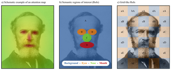
Figure 1.
Alternative ways to determine the similarity between eye movement sequences. a) Fixation density can be plotted as an attention map (Caldara & Miellet, 2011). Correlations between attention maps can be used as a measure of similarity. b,c) An image can be divided into regions of interest (RoIs) based on the semantic properties of the image (b) or based on a grid (c). Using these RoIs, eye movement sequences can be re-coded as character strings, and a string edit distance can be used as a similarity measure (Cristino et al., 2010; Levenshtein, 1966; West et al., 2006).
The downside of attention maps is that they contain no representation of fixation order. One can circumvent this limitation by analysing subsequent time-windows separately (e.g., Grindinger et al., 2011). But, from a practical point of view, the minimum size of the time-window is constrained by the need to maintain a sufficient number of fixations in each temporal bin. Therefore, attention maps are, in most cases, sub-optimal if one is interested in the temporal properties of eye movement sequences.
String edit methods. String edit methods are traditionally the most common way to determine the similarity between eye movement sequences (Brandt & Stark, 1997; Cristino et al., 2010; Duchowski et al., 2010; Foulsham & Underwood, 2008; Hacisalihzade et al., 1992; Privitera & Stark, 2000; West et al., 2006; Zangemeister & Oechsner, 1996). In this approach, pioneered by Hacisalihzade, Stark, and Allen (1992), eye movement sequences are recoded as character strings. In order to make this possible, the image is segregated into different regions of interest (RoIs). This can be done based on the semantic properties of the image (Figure 1b). For example, for the picture of a face it would make sense to divide the image into at least four RoIs, corresponding to the eyes, nose, mouth, and background respectively. Alternatively, the image can be divided into a grid, in which case no assumptions have to be made about the most sensible semantic segregation of the image (Figure 1c). Finally, some authors have proposed a data-driven way to define RoIs automatically. This can be done post-hoc, based on the viewing patterns of the participants, or beforehand, based on an analysis of the image (e.g., Privitera & Stark, 2000).
The next step is to re-code the eye movement sequence as a string of characters. Let's consider the following eye movement sequence:
eyes → nose → mouth → eyes
Given the RoIs from Figure 1b, the corresponding character string would be:
BCDB
After re-coding, all that is needed is a suitable similarity measure for character strings, for which there are many well-established algorithms. The best known of these are the Levenshtein distance (Levenshtein, 1966) and its numerous variations (Okuda, Tanaka, & Kasai, 1976; Wagner & Lowrance, 1975; Zangemeister & Liman, 2007).
In its simplest form, (i.e., the unmodified Levenshtein distance; Levenshtein, 1966), the string edit method suffers from a number of severe drawbacks. Specifically, it does not take into account factors such as fixation duration, nor the fact that RoIs are usually not 'equally unequal' (e.g., given the RoIs from Figure 1c, 'aA' is more similar to 'bA' than to 'cF'). We have recently proposed a string edit method, based on the Needleman-Wunsch algorithm (Needleman & Wunsch, 1970), in which most of these issues have been resolved (Cristino et al., 2010). This new method, which we called 'ScanMatch', is substantially more sensitive than the traditional string edit methods. But there are more general concerns that are not easily addressed within the constraints imposed by the string edit framework.
For example, any string edit method requires an image to be divided into RoIs. It can be difficult, or prohibitively time consuming, to define semantic RoIs (Figure 2), and the validity of data-driven/ artificial RoIs (Privitera & Stark, 2000) has been questioned (Grindinger et al., 2011). As a result, some researchers prefer to use grid-like RoIs (Figure 1c). In this case the RoIs serve as a proxy for a low-resolution coordinate system, and there may be significant advantages to using a more natural, geometric representation.
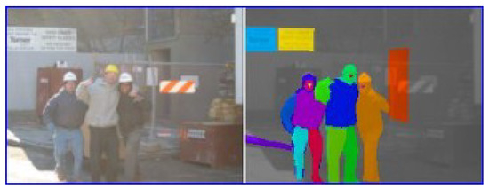
Figure 2.
The LabelMe website allows visitors to define semantic RoIs (indicated by the coloured areas in the right pane) in an image (Russel, Torralba, & Murphy, 2008), thus using crowd-sourcing to overcome the difficulties inherent to semantic RoIs.
Geometric methods. In geometric (or dimensional) methods, eye movements are represented by their geometric properties (location, saccade direction, fixation duration, etc.). This stands in contrast with the statistical approach of attention maps, and the RoI approach of string edit methods.
Zangemeister and Oechsner (1996) and, more recently, Jarodzka et al. (2010) have proposed algorithms that are essentially intermediates between string edit methods and geometric methods. In this approach, eye movement sequences are represented by series of vectors that represent (usually) the direction and amplitude of a saccade. But the approach is similar in spirit to string editing through its use of alignment (cf. Needleman & Wunsch, 1970): Series of vectors that line up well are considered similar. This method has the advantage of doing away with the awkward need for RoIs and re-coding schemes. In addition, Jarodzka et al.'s (2010) algorithm has an interesting property: It allows researchers to determine different similarity measures that each focus on a different aspect of the eye movements (e.g., shape, position, or length). Whether this is a feature or a limitation depends on the goals and prior knowledge of the researcher. It is a feature when a researcher has a specific hypothesis about the dimensions that he or she expects to be most relevant. It is a limitation in exploratory research, when a firm hypothesis is lacking.
Mannan et al. (1995, 1997; see also Henderson et al., 2007) have proposed a 'nearest neighbour' method that is conceptually most similar to the method that we will propose in the present paper, albeit less flexible. Mannan et al. (1995) represent eye movement sequences as sets of fixations (i.e., x, y coordinate pairs). Each fixation is mapped onto the nearest fixation from the other set. This results in a large number of mappings, each associated with a mapping distance. The (overall) distance is the sum of all mapping distances (after normalizing for the length of the eye movement sequences).
A clever variation on this approach has been described by Dempere-Marco et al. (2006), who used the earth mover distance (EMD) or Wasserstein metric. The EMD is generally conceptualized as the amount of traffic that is required to fill a set of holes (the fixations in sequence A) with a set of dirt piles (the fixations in sequence B). The advantage of this approach over a point-mapping rule, such as the one used by Mannan et al. (2006), is that it allows one to take fixation duration into account: Long fixations correspond to deep holes or large piles of dirt.
The methods of Mannan et al. (1995) and Dempere-Marco et al. (2006) do not require re-coding and RoIs. However, the drawback of these methods is that they do not take fixation order into account. The similarity measure that we will propose here can be viewed as a simplified, multidimensional variation on the method developed by Mannan et al. (1995, 1997).
The proposed similarity measure
Representation
Sets of fixations. We represent eye movements sequences as sets of fixations. Each fixation is defined by an arbitrary number of dimensions. For example, a fixation may be defined only by its location, in which case it has two dimensions (x, y). (Assuming that we do not take vergence into account, otherwise there would be a z dimension as well.) But in principle any number and combination of dimensions can be used, which is the primary departure from Mannan et al.'s method (1995, 1997). For example, in many situations it would make sense to define fixations by their location, timestamp and duration, in which case there would be four dimensions (x, y, t, d). Note that, unlike in Jarodzaka et al.'s (2010) method, the set of fixations is unordered. Nevertheless, the temporal properties of an eye movement sequence can be readily taken into account by incorporating temporal dimensions such as time and fixation duration.
Using eye tracker output. The benefit of this representation is that it closely matches the output from most eye trackers, which generally (although not always) offer an abstraction layer in which individual gaze samples are converted into larger-scale events, such as fixations and saccades. For example, in the raw data produced by the Eyelink series of eye trackers (SR Research, Mississauga, ON, Canada), fixations look like this:
EFIX L 16891857 16893183 1327 32.7 369.28588
Or, more schematically:
EFIX [eye] [start time] [end time] [duration] [x] [y] [pupil size]
The relevant dimensions can be easily extracted from this type of raw data, and no elaborate re-coding scheme will usually be required.
Data 'whitening'. However, one situation in which some pre-processing is required is when you want to incorporate dimensions that lie on qualitatively different scales.
To illustrate this point, let's consider the following example: We use location and fixation duration (x, y, d) as dimensions. We use seconds as units for d and pixels as units for x and y. This means that values for d will generally be small (below one), whereas values for x and y will be large (range in the hundreds). More precisely, the problem is that d has less variance than x and y. Because of this imbalance, d will contribute little to the distance measure.
This problem can be resolved through a process called 'whitening': For each dimension, all values are divided by the standard deviation of values within that dimension. As a result of this scaling operation, all dimensions will have unit variance, and will contribute equally to the distance measure.
It is difficult to say whether or not whitening should be applied in a given situation, because it is not necessarily beneficial when applied inappropriately. It may be desirable for some dimensions to have a relative large variance. For example, when you increase the length of an eye movement sequence, the variance in time (t) will increase, but the variance in position (x, y) may not. In this case, the difference in variance between dimensions may be informative, and should not be undone through whitening. Conversely, the value on a particular dimension may be essentially constant (for example the y coordinate if participants are following a horizontally moving dot), except for noise. If this is the case, whitening is undesirable, because it will have the effect of amplifying noise.
Given these considerations, we propose, as a rule of thumb, not to apply whitening unless some dimensions are obviously incomparable (i.e., the standard deviation differs more than an order of a magnitude between dimensions), or if there is a theoretical reason why variance should be strictly equal across dimensions.
Distance measure
Rationale. The goal of the proposed distance measure is to take two eye movement sequences, which we will call S and T, and return a value that estimates the distance (i.e., the inverse of the similarity) between S and T.
We propose that the best way to achieve this is by constructing a mapping between S and T, so that each point (i.e., fixation) from S is mapped onto at least one point from T, and vice versa. The goal is to minimize the (normalized) sum of the distances associated with all mappings (Figure 3a).
This 'mapping problem' has no known solution that is both efficient and guaranteed to be optimal, but there are various heuristic that consistently achieve a very good mapping. In preliminary analyses we have explored a number of different heuristics and have found that 'double-mapping' is the preferred technique, because it is computationally cheap and not notably, if at all, less accurate than more sophisticated heuristics (cf. Mannan et al., 1995).
In the double mapping technique, each point from S is mapped onto the nearest neighbour from T. In addition, each point from T is mapped onto the nearest neighbour from S (Figure 3b). Many mappings thus occur twice. Importantly, double mapping does not suffer from complex problems such as the need to split long mappings into multiple shorter ones, or pruning of spurious mappings.
As noted by Henderson et al. (2007), double-mapping has the risk of mapping a large number of points from S onto a single point (or small number of points) from T. This is true, but in general we prefer the double-mapping approach over the 'unique assessment' mapping rule proposed by Henderson et al. (2007). This is because, unlike unique assessment, double-mapping does not require an equal number of points in each set (i.e., eye movement sequences of different lengths can be compared), and therefore allows for a broader application.
Algorithm. A point-mapping is the mapping between a point p in S and a point q in T, and is associated with a distance, d(p,q), which is the Euclidean distance between p and q:
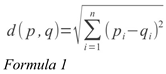
Here, n is the number of dimensions, and pi and qi are the i-th dimension of p and q, respectively.
A sequence-mapping between S and T is the collection of all point-mappings. Following the double-mapping technique, all points from S are mapped onto their nearest neighbour in T, and vice versa. A sequence-mapping is also associated with a distance, D(S,T), which is the normalized sum of all the point-mapping distances. Normalization occurs by dividing D(S,T) by the number of points in the largest sequence. This prevents long sequences from being unfairly penalized:
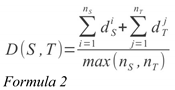
Here, nS is the length of S, nT is the length of T, di is the distance between point i in S to its nearest neighbour in T, dj is the distance between point j in T to its nearest neighbour in S, and D(S,T) is the distance between S and T.
A different, and perhaps more intuitive, way of describing the algorithm is through pseudo-code. The equivalent pseudo-code is as follows:
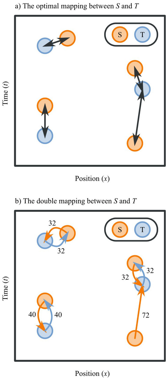
Figure 3.
A schematic illustration of the mapping principle. For display purposes, only two dimensions (x, t) are shown, but the principle generalizes to an arbitrary number of dimensions (Formula 1). a) The optimal mapping between S and T. b) The double mapping, which is a good and computationally cheap approximation of the optimal mapping. In this example, we can determine the distance between S and T as follows (applying Formula 2):
D(S,T)=(32+32+40+40+32+32+72)/max(3,4)
D(S,T)=70
D = 0For all points p in S:Find nearest point q in TD = D + distance(p,q)For all points q in T:Find nearest point p in SD = D + distance(p,q)D = D / max(size(S),size(T))
Again, S and T denote two eye movement sequences, p and q denote points in S and T respectively, distance() is the Euclidean distance function, and D is the resulting distance.
Implementation. We have developed an optimized Python (Jones, Oliphant, & Peterson, 2001; Van Rossum, 2008) implementation of the algorithm, which can be obtained from http://www.cogsci.nl/eyenalysis. In addition to the algorithm per se, this implementation provides functionality for reading text data, whitening data, cross-comparing large datasets, and performing k-means cluster analyses. Documentation and demonstration scripts are included.
As of yet, the algorithm has not been implemented in other programming languages. However, as is apparent from the pseudo-code shown above, implementing the algorithm is trivial in most languages, particularly those that have strong matrix- and data-manipulation capabilities, such as Python, R (R Development Core Team, 2010), and MATLAB (The MathWorks, 1998) / Octave (Eaton, 2002).
Effects of sequence length, dimensionality, and spacing
An important limitation to keep in mind when applying a distance measure, such as the one proposed here, is that distance ratings are only meaningful within a particular set of data—Distance ratings do not have an absolute meaning.
To illustrate this, we calculated the mean distance between randomly generated sequences (N=1000 for each data-point). This was done with various numbers of dimensions (1, 2, 4, 8, and 16) and with various sequence lengths (1-32). We also varied 'fixation spacing', by which we mean the following: In the fixed space condition (Figure 4a) coordinates had random values between 0 and 1. In the growing space condition (Figure 4b), coordinates had random values between 0 and X, where X was equal to the sequence length. In other words, the fixed space condition simulated a situation in which gaze is strictly confined, whereas the growing space condition simulated a situation in which the eyes roam free, inspecting an ever growing area.
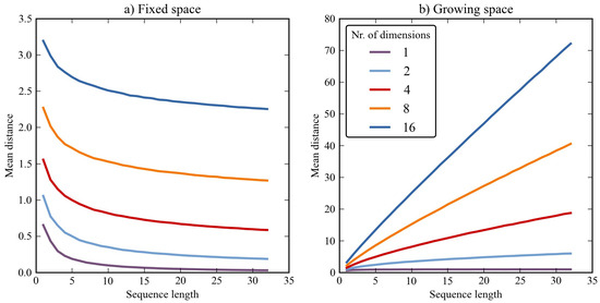
Figure 4.
The mean distance between two randomly generated sequences as a function of dimensionality, sequence length, and spacing. a) Values were randomly chosen between 0 and 1. b) Values were randomly chosen between 0 and X, were X is equal to the sequence length.
The effect of dimensionality is clear (Figure 4). Increasing the number of dimensions leads to higher distance ratings. This is not surprising, because, in a sense, the Euclidean distance function (Formula 1) does not fully normalize for dimensionality. This can be intuitively shown with an example: Opposite corners of a cube (three dimensions) are further apart than opposite corners of a square (two dimensions), provided that the length of the edges is kept constant.
More surprising perhaps, is that the effect of sequence length is variable. Specifically, it depends on whether fixations are spaced within a fixed region (Figure 4a) or a region that expands as the number of fixations increases (Figure 4b). This is a result of the normalization procedure (Formula 2). If fixations are spaced within a fixed region, normalization over-compensates, and the mean distance rating decreases with increasing sequence length. If, on the other hand, fixations are spaced within in a region that grows as the number of fixations increases (Figure 4b), normalization under-compensates and the mean distance rating increases with sequence length.
This simulation illustrates that normalization for sequence length is inherently problematic. If the point of gaze is strictly confined within a fixed region, the optimal normalization procedure is different from when gaze is allowed to roam completely free. In practice, one may observe any intermediate between these two extremes: As people scan an image, their eyes will sequentially inspect different locations, and thus the region that contains fixations will grow over time. But, at the same time, gaze is restricted by factors such as screen boundaries, so the region that contains fixations cannot grow indefinitely.
In summary, distance ratings are relative and do not carry meaning outside of a particular dataset. With respect to the distance measure proposed here, mean distance ratings are affected by the number of dimensions, the (average) sequence length, and, more subtly, the way in which fixations are spread out over space, time, and other dimensions.
Experiment
We have conducted an experiment to compare the sensitivity of the proposed algorithm, Eyenalysis, to that of existing algorithms. Specifically, we compared Eyenalysis to ScanMatch (Cristino et al., 2010) and the Levenshtein distance (Levenshtein, 1966). The reason for choosing these two algorithms as points of reference is that they represent both the traditional (the Levenshtein distance) and state-of-the-art (ScanMatch) in similarity measures.
The term 'sensitivity' requires some clarification in this context. Essentially, we define sensitivity operationally as how well a similarity measure deals with noise in experiments such as the present one.
We generated a large number of artificial, yet realistic eye movement sequences that fell into two categories. Next, we performed a cross-comparison of this dataset (using a similarity measure), and performed a k-means cluster analysis on the resulting cross-comparison matrix. This yielded two clusters of eye movement sequences. Our measure of interest is how well the two clusters, which have been generated in a data-driven way, match the two given categories (i.e., the 'real' clustering).
In situations with very little noise (i.e., highly distinct categories) we expect any sensible similarity measure to perform perfectly. In situations with very high levels of noise, we expect any similarity measure to perform at chance level. However, the amount of noise that a similarity measure is able to cope with is taken as a measure of its sensitivity.
In the present experiment, the data-set is three-dimensional, containing the position (x, y) and time-stamp (t) of each fixation. We chose this representation, because it is a natural and common way to represent eye movement data, and because it allows for a straight-forward comparison to ScanMatch and the Levenshtein distance. However, in Eyenalysis all dimensions are treated in the same way, regardless of the type of information that they convey. So the labels that we have attached to the dimensions are, in a sense, arbitrary.
All scripts, input data, and output data are available from http://www.cogsci.nl/eyenalysis.
Data generation procedure
Generating artificial eye movement sequences. As a starting point, we took two images (Figure 6a,b). Using the iLab Neuromorphic vision toolkit (Itti & Koch, 2000; Itti, Koch, & Niebur, 1998), we generated an artificial eye movement sequence, consisting of 10 saccades (11 fixations), for each of the two images. Each fixation was defined by a timestamp (t) and a position (x, y).
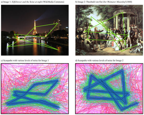
Figure 6.
a,b) Two images were used to generate realistic, artificial eye movement data using the iLab Neuromorphic vision toolkit (Itti & Koch, 2000; Itti et al., 1998). c,d) Different levels of noise (indicated by different colours) were added to the eye movement sequences from (a,b).
For 200 levels of noise (σ from 0 to 1990 in steps of 10; in px for x, y; in ms for t) we did the following: The two sequences were copied 50 times and noise was added to each copy (Figure 6c,d; Figure 5). Specifically, a random value (sampled from a normal distribution with µ = 0 and σ per the noise level) was added to x, y, and t for all fixations. x was constrained between 0 and 1280 (the width of the images), y between 0 and 960 (the height of the images), and t between 0 and 5000. For each fixation there was a probability of σ/4000 of either an omission or an addition. An omission meant that the fixation was skipped. An addition meant that the fixation was followed by a new, completely random (within the given constraints) fixation.
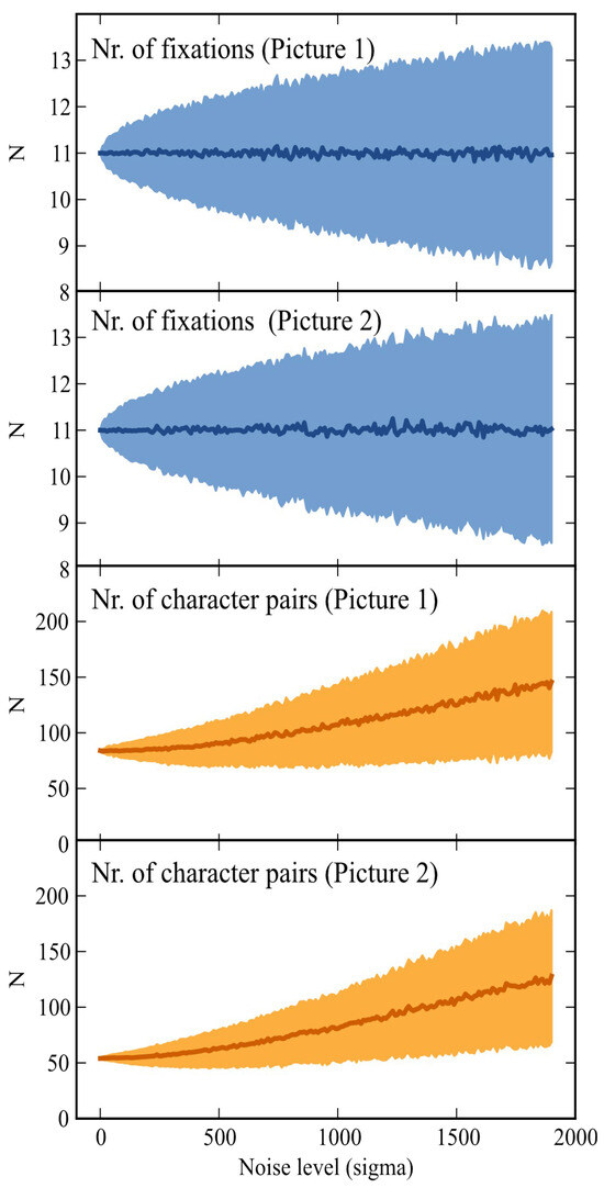
Figure 5.
Descriptive statistics (the shaded area indicates the standard deviation) for the artificial eye movement data. Whereas the average number of fixations is relatively constant across noise levels and the two pictures, the average length of the character strings increases. This is because the length of the character strings also reflects the duration of the fixations.
Character string representation. Because the Levenshtein distance (Levenshtein, 1966) and ScanMatch (Cristino et al., 2010) require input in the form of character strings, the eye movement sequences were re-coded as character strings. Each fixation was coded as a pair of characters (e.g., aA), where the first character represents x and the second character represents y. This representation was chosen for compatibility with ScanMatch (Cristino et al., 2010). As described below, we used a slightly modified version of the Levenshtein distance (Levenshtein, 1966), to overcome its single-character (or 26 RoIs) limit. t was represented as repetition of a character-pair (Figure 5). For each 100ms, a character-pair was repeated. So, for example, a 350 millisecond fixation in the upper-left of the image would be represented as:
aAaAaA
Analysis
For each algorithm (ScanMatch, Levenshtein distance, and Eyenalysis) and noise level (0 to 1990) we performed the following analysis:
Each movement sequence was compared to each other eye movement sequence. This resulted in a 100x100 matrix of distance scores. Using the PyCluster package (de Hoon, Imoto, & Miyano, 2010), a 1-pass k-means cluster analysis was performed on the cross-comparison matrix to obtain 2 clusters.
Clustering accuracy and chance level. The clusters determined by k-means clustering are unlabelled, in the sense that it is not defined which cluster (kmeansA or kmeansB) matches which image (imageA or imageB). We therefore first determined the clustering accuracy assuming that kmeansA maps onto imageA, and reversed this mapping if the clustering accuracy was less than 50%. Because this approach prevents accuracy from dropping below 50%, we needed to explicitly determine chance level. An analysis using random data set chance level at 54%.
Application of ScanMatch. A 26x26 grid ('number of bins') with an RoI modulus of 26 was used. A substitution matrix threshold of 19 was used, which was 2 times the standard deviation of the 'gridded' saccade size (cf. Cristino et al., 2010). The gap value and temporal binsize were left at 0. Because all parameters were either derived from the data in a predetermined manner, or left at their default value, there were no free parameters in our application of ScanMatch.
Application of Levenshtein distance. We used the classic Levenshtein distance (Levenshtein, 1966), with two modifications to allow for a more straight-forward comparison to the other algorithms. Firstly, we used character-pairs, rather than single characters, as units for matching. This was done so that we could use the same dataset as input for both ScanMatch (Cristino et al., 2010) and the Levenshtein distance. Secondly, the resulting distance-score was normalized by dividing the score by the length of the largest eye movement sequence. This normalization procedure is not part of the Levenshtein distance per se, but is commonly applied when used in eye movement research (e.g. Foulsham & Underwood, 2008). There were no free parameters in our application of the Levenshtein distance.
Application of Eyenalysis. Eyenalysis was applied on both the raw dataset and on the whitened data, as outlined in the section Data 'whitening'. There were no free parameters in our application of Eyenalysis.
Results
The results of the experiment are shown in Figure 7. In line with Cristino et al. (2010), we found that the Levenshtein distance (Levenshtein, 1966), despite being a widely used method, offers poor performance relative to the other methods that we tested (Figure 7a,b).
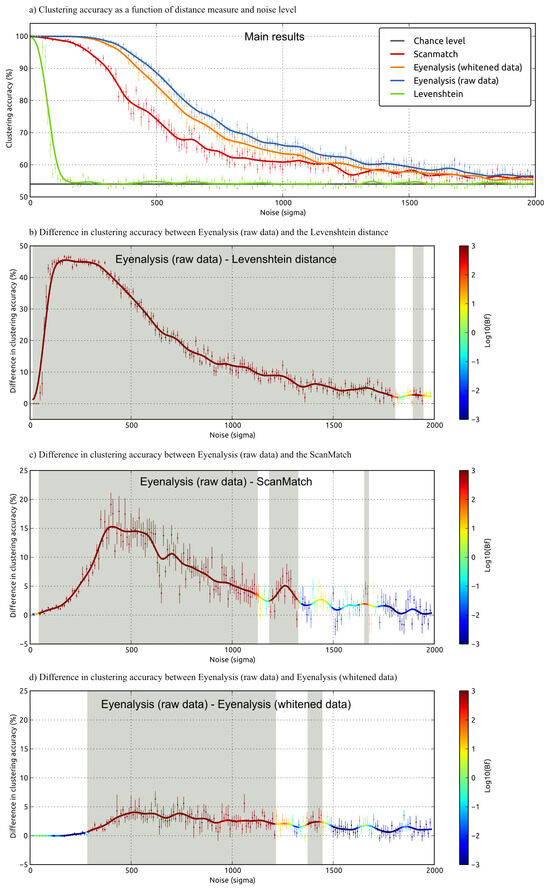
Figure 7.
Results of the experiment. a) Clustering accuracy as a function of method and noise level. b,c,d) The difference in clustering accuracy between Eyenalysis (raw data) and the Levenshtein distance (Levenshtein, 1966) (b), Scan-Match (Cristino et al., 2010) (c), and Eyenalysis (whitened data) (d). Error bars represent the standard error. In (b,c,d) the colour coding reflects the Bayes factor (Bf), using a Bayesion sliding window (The Bayes factors (Bfs) shown in Figure 7b,c,d are calculated using the following 'sliding window' technique: First, a Bf was calculated for each data-point, assuming a uniform distribution for the expected difference, with a lower bound of 0% and an upper bound of 46% (i.e., 100% - chance level). Next, the Bfs were smoothed using a Hanning window of width 70). Data points where Bf > 100 (i.e., ‘decisive evidence’ for a difference, cf. Wetzels et al., 2011) are marked with a light-gray background. All lines have been smoothed using a Hanning window of width 70.
Discussion
We have proposed Eyenalysis, a novel algorithm to estimate the similarity between eye movement sequences. Using realistic artificial eye movement data, we have shown that Eyenalysis is more sensitive, at least in the present experiment, than the commonly used Levenshtein distance (Levenshtein, 1966) and ScanMatch (Cristino et al., 2010), an advanced string edit measure that we have previously proposed to overcome the limits of traditional string edit methods.
With an eye towards an application in real-life experimental settings, an important feature of Eyenalysis is its simplicity. Applying the algorithm is straight-forward, and does not require re-coding eye movement data into a special format, such as a character string representation. A Python implementation is provided, but the algorithm can easily be implemented from scratch in any programming language.
A landmark study by Noton and Stark (1971) illustrates how similarity measures can be used to elucidate theoretical issues. Noton and Stark (1971) noted that people tend to scan images in a stereotyped way. That is, the eye movement sequence of a person is relatively constant across multiple viewings of the same image (but not across different people, or across different images). Based on this finding, they proposed that eye movement sequences are an integral part of memory. By consistently viewing the same scene in (more or less) the same way, one can predict the visual input that is expected on each fixation. Therefore, so Noton and Stark (1971) argued, stereotyped eye movements could facilitate recognition.
Although their results were convincing, Noton and Stark (1971) did not perform a rigorous analysis. The similarities were obvious on visual inspection of the data (but see Privitera & Stark, 2000 for a more recent, quantitative corroboration). However, in some cases, for example when the data-set is large or noisy, a quantitative similarity measure, such as the one proposed here, is required. More specifically, a similarity measure can help researchers to address a particular, very common class of research questions. For example, one can estimate whether there are differences between predetermined groups of eye movement sequences (e.g., corresponding to different experimental conditions). Or, when combined with a cluster analysis, one can split a large set of eye movement data into groups of more-or-less homogeneous eye movement sequences in a data-driven way (also see Duchowski et al., 2010 and Privitera & Stark, 2000 for sophisticated similarity-based analyses).
The usefulness of similarity measures has been long recognized, and quite a few different methods have been proposed (Caldara & Miellet, 2011; Cristino et al., 2010; Dempere-Marco et al., 2006; Duchowski et al., 2010; Gibboni et al., 2009; Grindinger et al., 2011; Jarodzka et al., 2010; Levenshtein, 1966; Mannan et al., 1995, 1997; Privitera & Stark, 2000; West et al., 2006). Although some methods are more sensitive than others, many are useful in practice (Foulsham & Underwood, 2008; Henderson et al., 2007), and the choice for a specific algorithm depends largely on the goals of the researcher.
Eyenalyis is particularly well suited for exploratory analyses, because it allows one to simultaneously include many different factors in the analysis, and does not require the expected differences to be specified a priori. The algorithms proposed by Mannan et al. (1995, 1997; see also Henderson et al., 2007) and Dempere-Marco et al. (2006) are very similar to Eyenalysis when only positional information is considered. The primary contribution of Eyenalysis is to make it possible to include an arbitrary number and combination of dimensions. Any property of a fixation can be included in the analysis, provided that a numerical value can be assigned to it.
But there are also a number of limitations. As noted in the introduction, it is difficult to interpret similarity ratings obtained from Eyenalysis (and to some extent this is true of all similarity ratings). Consider, for example, an experiment in which you expect two groups to differ in the latencies of their saccadic eye movements. The problem with using a similarity measure in this case is that, even if you find a difference between the groups (i.e., eye movement sequences are more similar within groups than between groups), you cannot be sure that this difference is indeed driven primarily by a difference in saccadic latencies. Therefore, additional analyses may be required to interpret the similarity ratings.
Another limitation has to do with the relative weights that are assigned to each dimension (position, time, fixation duration, etc.). Weighting dimensions is straight-forward. If you want a dimension to exert a larger influence on the similarity rating, you multiply all values in that dimension by some factor larger than 1. Conversely, the importance of a dimension can be reduced by multiplying all values by a factor between 0 and 1. But the difficulty lies in deciding on an appropriate weighting. This is essentially a conceptual problem that revolves around the proper definition of 'similarity': Is a distance of 100px comparable to an interval of 10ms, 100ms, or 1000ms? At present, there is no satisfactory solution to the issue of dimensional weighting, particularly when dimensions with incomparable units (e.g., pixels and milliseconds) are incorporated. As a rule of thumb, we propose that the variance within dimensions should be kept relatively constant. If this is not the case, a 'whitening' procedure can be performed, as described in the section Data 'whitening'.
An important feature of Eyenalysis is that it does not require an image to be segmented into RoIs. This is beneficial when such segmentation is difficult. But when RoIs are available, particularly semantically defined RoIs, this is a limitation. In such cases, a string edit algorithm is the method of choice. Among currently available string edit methods, ScanMatch (Cristino et al., 2010) is most sensitive, and should therefore be preferred over the classic Levenshtein distance (Levenshtein, 1966). Another useful feature of ScanMatch is that you can specify relationships between points in an image that violate geometric constraints (e.g., A→B > B →A), which is not possible in a geometric approach.
In summary, similarity measures are a powerful tool for eye movement research. We have proposed and validated a simple, yet sensitive algorithm for estimating the similarity between a pair of eye movement sequences.
Acknowledgments
This research was funded by a grant from NWO (Netherlands Organization for Scientific Research), grant 463-06-014 to Jan Theeuwes, and the ESRC Bilateral Grant Scheme to Iain D. Gilchrist and Jan Theeuwes.
References
- Brandt, S. A., and L. W. Stark. 1997. Spontaneous eye movements during visual imagery reflect the content of the visual scene. Journal of Cognitive Neuroscience 9, 1: 27–38. [Google Scholar] [CrossRef] [PubMed]
- Caldara, R., and S. Miellet. 2011. iMap: a novel method for statistical fixation mapping of eye movement data. Behavior Research Methods 43, 3: 864–878. [Google Scholar] [CrossRef]
- Cristino, F., S. Mathôt, J. Theeuwes, and I. D. Gilchrist. 2010. ScanMatch: A novel method for comparing fixation sequences. Behavior Research Methods 42, 3: 692–700. [Google Scholar] [CrossRef]
- de Hoon, M., S. Imoto, and S. Miyano. 2010. The C Clustering library. Retrieved from http://bon- sai.hgc.jp/~mdehoon/software/cluster/software.htm.
- Dempere-Marco, L., X. P. Hu, S. M. Ellis, D. M. Hansell, and G. Z. Yang. 2006. Analysis of visual search patterns with EMD metric in normalized anatomical space. IEEE Transactions on Medical Imaging 25, 8: 1011–1021. [Google Scholar] [CrossRef] [PubMed]
- Duchowski, A. T., J. Driver, S. Jolaoso, W. Tan, B. N. Ramey, and A. Robbins. 2010. Scanpath comparison revisited. In Proceedings of the 2010 Symposium on Eye-Tracking Research & Applications. New York, NY: ACM: pp. 219–226. [Google Scholar]
- Eaton, J. W. 2002. GNU Octave Manual. Network Theory Limited. [Google Scholar]
- Foulsham, T., and G. Underwood. 2008. What can saliency models predict about eye movements? Spatial and sequential aspects of fixations during encoding and recognition. Journal of Vision 8, 2: 1–17. [Google Scholar]
- Gibboni, R. R., P. E. Zimmerman, and K. M. Gothard. 2009. Individual differences in scanpaths correspond with serotonin transporter genotype and behavioral phenotype in rhesus monkeys (macaca mulatta). Frontiers in Behavioral Neuroscience 3, 50: 1–11. [Google Scholar] [CrossRef]
- Grindinger, T., V. Murali, S. Tetreault, A. Duchowski, S. Birchfield, and P. Orero. 2011. Algorithm for discriminating aggregate gaze points: comparison with salient regions-of-interest. In Proceedings of the 2010 international conference on computer vision. Berlin, Germany: Springer-Verlag: pp. 390–399. [Google Scholar]
- Hacisalihzade, S. S., L. W. Stark, and J. S. Allen. 1992. Visual perception and sequences of eye movement fixations: A stochastic modeling approach. IEEE Transactions on systems, man, and cybernetics 22, 3: 474–481. [Google Scholar] [CrossRef]
- Henderson, J. M., J. R. Brockmole, M. S. Castelhano, M. Mack, M. Fischer, W. Murray, and R. Hill. 2007. Edited by R. P. G. van Gompel, M. H. Fischer, W. S. Murray and R. L. Hill. Visual saliency does not account for eye movements during visual search in real-world scenes. In Eye movements: A window on mind and brain. Amsterdam, Netherlands: Elsevier: pp. 537–562. [Google Scholar]
- Itti, L., and C. Koch. 2000. A saliency-based search mechanism for overt and covert shifts of visual attention. Vision Research 40: 1489–1506. [Google Scholar]
- Itti, L., C. Koch, and E. Niebur. 1998. A model of saliency-based visual attention for rapid scene analysis. IEEE Transactions on Pattern Analysis and Machine Intelligence 20, 11: 1254–1259. [Google Scholar] [CrossRef]
- Jarodzka, H., K. Holmqvist, and M. Nyström. 2010. A vector-based, multidimensional scanpath similarity measure. In Proceedings of the 2010 sympsosium on eye-tracking research & applications. Austin, TX: ACM: pp. 211–218. [Google Scholar]
- Jones, E., T. Oliphant, and P. Peterson. 2001. Scipy: Open source scientific tools for Python. Retrieved from http://www.scipy.org/.
- Levenshtein, V. I. 1966. Binary codes capable of correcting deletions, insertions, and reversals. Soviet Physics Doklady 10, 8: 707–710. [Google Scholar]
- Mannan, S. K., K. H. Ruddock, and D. S. Wooding. 1995. Automatic control of saccadic eye movements made in visual inspection of briefly presented 2-D images. Spatial Vision 9, 3: 363–386. [Google Scholar] [PubMed]
- Mannan, S. K., K. H. Ruddock, and D. S. Wooding. 1997. Fixation patterns made during brief examination of two-dimensional images. Perception 26: 1059–1072. [Google Scholar] [CrossRef]
- Needleman, S. B., and C. D. Wunsch. 1970. A general method applicable to the search for similarities in the amino acid sequence of two proteins. Journal of Molecular Biology 48, 3: 443–453. [Google Scholar] [CrossRef] [PubMed]
- Noton, D., and L. Stark. 1971. Scanpaths in eye movements during pattern perception. Science 171, 3968: 308–311. [Google Scholar] [CrossRef]
- Okuda, T., E. Tanaka, and T. Kasai. 1976. A method for the correction of garbled words based on the Levenshtein metric. IEEE Transactions on Computers 100, 2: 172–178. [Google Scholar]
- Privitera, C. M., and L. W. Stark. 2000. Algorithms for defining visual regions-of-interest: Comparison with eye fixations. IEEE Transactions on Pattern Analysis and Machine Intelligence 22, 9: 970–982. [Google Scholar] [CrossRef]
- R Development Core Team. 2010. R: A language and environment for statistical computing. Retrieved from http://www.R-project.org/.
- Russell, B. C., A. Torralba, K. P. Murphy, and W. T. Freeman. 2008. LabelMe: a database and web-based tool for image annotation. International Journal of Computer Vision 77, 1: 157–173. [Google Scholar]
- San Agustin, J., H. Skovsgaard, E. Mollenbach, M. Barret, M. Tall, D. W. Hansen, and J. P. Hansen. 2010. Evaluation of a low-cost open-source gaze tracker. In Proceedings of the 2010 Symposium on Eye-Tracking Research & Applications. Austin, TX: ACM: pp. 77–80. [Google Scholar]
- The MathWorks. 1998. MATLAB User's Guide. Natick, MA: Mathworks. [Google Scholar]
- Van Rossum, G. 2008. Python reference manual. Python software foundation. [Google Scholar]
- Wagner, R. A., and R. Lowrance. 1975. An extension of the string-to-string correction problem. Journal of the ACM 22, 2: 177–183. [Google Scholar]
- West, J. M., A. R. Haake, E. P. Rozanski, and K. S. Karn. 2006. eyePatterns: software for identifying patterns and similarities across fixation sequences. In Proceedings of the 2006 symposium on Eye tracking research & applications. San Diego, CA: ACM: pp. 149–154. [Google Scholar] [CrossRef]
- Wetzels, R., D. Matzke, M. D. Lee, J. N. Rouder, G. J. Iverson, and E.-J. Wagenmakers. 2011. Statistical evidence in experimental psychology. Perspectives on Psychological Science 6, 3: 291–298. [Google Scholar] [CrossRef]
- Zangemeister, W. H., and T. Liman. 2007. Foveal versus parafoveal scanpaths of visual imagery in virtual hemianopic subjects. Computers in Biology and Medicine 37, 7: 975–982. [Google Scholar] [CrossRef]
- Zangemeister, W. H., and U. Oechsner. 1996. Evidence for scanpaths in hemianopic patients shown through string editing methods. Advances in Psychology 116: 197–221. [Google Scholar]
Copyright © 2012. This article is licensed under a Creative Commons Attribution 4.0 International License.