1. Introduction
There are many works on designing control strategies for robotic manipulators with standard and broader approaches [
1,
2,
3,
4], but newer and more specialized control strategies are still being developed [
5,
6], with many experts on this topic in the academic and private sectors involved. A lot of papers are also focused on using robotic manipulators as a black-boxed motion mechanism for control of the end effector of the robot based on external sensors such as force and torque sensors [
7,
8,
9,
10], optical sensors and cameras [
11,
12], or accelerometers and other electrical sensors [
13,
14]. However, none of these works handle the response of the robotic manipulator to externally unstable and relatively fast processes, although the need for a robotic manipulator controlling such a process in an industrial environment may arise in the future with fast-developing technologies such as virtual and augmented reality with tactile feedback for teleoperation of robots [
15,
16,
17,
18,
19]. Remote-operated industrial robots are also on the rise, mostly in dangerous environments or remote locations such as offshore oil and gas platforms [
20,
21]. Self-motion of these robots is relatively important and can require more delicate tasks with more advanced algorithms supporting better stability of handled tasks. Although these applications do not control unstable processes, it can be assumed their development will lead to a broader scope of applications that may need such feedback control (see [
15]) in processes such as polishing, grinding, or deburring in human-robot collaboration tasks or many advanced applications requiring a non-standard approach to industrial robotic systems [
22].
Many different designs of B&P structures can be found in educational, research, or hobby projects, from the “classic” 2 degrees of freedom (DoF) design with actuators connected in series [
23,
24] or parallel [
25,
26] configuration to the 6 degrees of freedom parallel Stewart platform [
27,
28]. There are also several higher DoF solutions for actuators connected in series, such as [
29,
30,
31].
This vast range of solutions for B&P systems proves it is a very interesting and challenging problem to solve, and this thesis adds to this portfolio of electromechanical structures and their control to reach the goal of ball stabilization and trajectory tracking. Many B&P control solutions use standard PID control or state-space controllers and their variations (PD, LQR) [
25,
26,
27,
28]. Among the “non-standard” solutions are double feedback loop structures based on fuzzy logic [
32], fuzzy supervision and sliding control [
33], non-linear switching [
34], and the H-infinity approach [
35]. The control of the B&P model is tested in [
29] using a 7-degrees-of-freedom robotic manipulator (Robai Cyton Gamma 300), but only the last 2 axes are used for control and others are stationary. This decoupled design would not be able to perform the positioning of the plate in space or move the end effector to another location while still maintaining the correct control.
This paper aims to use the full extent of all seven axes; although several of them might be moving only slightly, they are still being used in kinematic calculations, and their dynamics influence the whole system. In addition, they can be used to move the whole plate in space while balancing the ball. The motivation is to extend current works on this topic to standard industrial serial manipulators while using all their joints in the control itself. An optimal controller algorithm is derived to have a better grasp of the control process with easily adjustable penalization of action value to reduce the load on the manipulator’s servos and gearboxes, which must be kept in mind while using the manipulator for longer periods. There are many references to the topic of B&P control, but most of them deal only with the quality of the control, neglecting the factor of the manipulator’s wear and tear.
2. Ball and Plate Mathematical Model
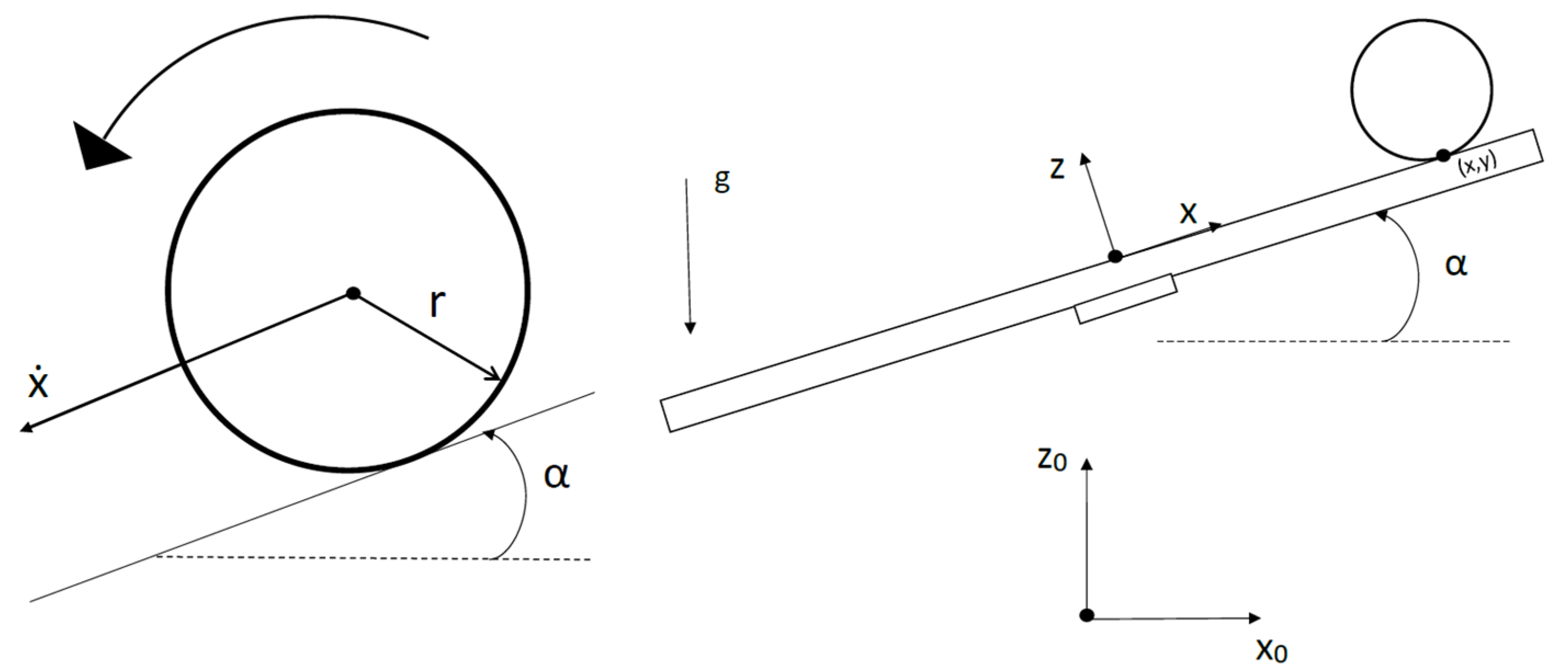
The best approach in the case of the B&P model is to divide it into two separate directional components, x and y. The model setup of such a system for one coordinate is depicted in
Figure 1, which describes the motion of a ball on a plate in one of these dimensions. The position of the ball (x, y [
m]) is expressed in the local coordinate system of the plate xz, defined in the right-handed Cartesian base frame x
0z
0. The plate can rotate around the center of this local coordinate system by the angle α (and β for a 2-dimensional system). The ball, described by its radius r [
m] and velocity ẋ [
ms−1], moves on the plate with gravitational acceleration g [
ms−2] acting on the ball.
This model is slightly simplified and does not show forces acting on the ball other than gravity. These forces (e.g., friction) are present but neglected in favor of simplification in following the mathematical description, which helps with its derivation and design of the controller. The following assumptions are considered, which simplify the model:
The air friction is neglected;
The friction between the ball and the plate is neglected;
The ball is a homogeneous, ideal sphere (or spherical shell);
The plate has no boundaries and stretches infinitely long;
There is always slip-free contact between the ball and the plate.
The simplified and linearized model, resulting from the Euler-Lagrange equation of the second kind, is:
where
α and
β are angles of the plate for
x and
y coordinates, respectively, and
Kb [
ms−2] is a constant of the ball dependent only on the type of the ball (a full or hollow sphere) and gravitational acceleration. Double-dot notation expresses the second-time derivation of a given coordinate. The linearization is assumed for the ball’s position near the center of the plate and takes into account the assumption of
sin(
α)
≈ α for small angles (<5°). These equations can be expressed in Laplace format with transfer functions
Gx and
Gy:
Which clearly shows that the Ball and Plate system is symmetric for both coordinates. This symmetry is broken for the robotic manipulator used in this paper and it is approximated with first order transfer function and combined with Equation (3), resulting in a mathematical description of the whole Ball and Plate system with dynamics of the manipulator included in both the continuous form
G(
s) and the discrete form
G(
z−1):
where
Kr is the gain of the robot system,
Tr is its time constant,
B(
z−1) and
A(
z−1) are the nominator and denominator polynomials of the whole system, and
bi and
ai are their respective coefficients. This discrete transfer function will be used later in the design of the controller.
3. Linear-Quadratic Polynomial Controller Design
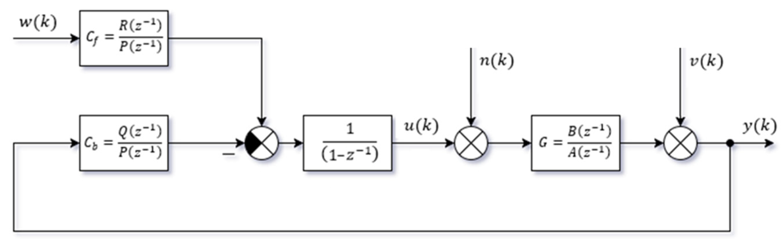
The controller designed in this paper has a 2-degrees-of-freedom structure (as seen in
Figure 2), with the feed-forward part
Cf acting as a filter for the reference value and responsible for reference tracking and the feed-back part
Cb responsible for stabilization and disturbance rejection. It also contains a summation part 1
/(1 −
z−1) and a controlled plant
G(
z−1). There are five signals present in the structure, namely the reference value
w(
k) (desired position of the ball), controller output
u(
k) (plate angle), the position of the ball
y(
k), and respective disturbances
n(
k) and
v(
k) acting on the system externally or through simplifications of the mathematical model.
The control law is derived from the linear-quadratic pole-placement control more closely described in [
36] and follows a minimization of the criterion
to obtain coefficients of the characteristic polynomial
D(
z−1) of the controller structure described in
Figure 2:
Parts of the criterion
e(
k) and
u(
k) are control error and controller output, respectively, and
qu is a penalization constant used to better control the influence of the controller output in this criterion. In
Figure 2,
B(
z−1) and
A(
z−1) are the nominator and denominator polynomials of the whole system, respectively, and
Q(
z−1) and
P(
z−1) are the nominator and denominator polynomials of controller
Cb. The degrees of these polynomials are directly dependent on the degrees of polynomials
B(
z−1) and
A(
z−1), which are more closely described in [
36]. For this specific case, where
∂B = 3 (degree of polynomial
B(
z−1)) and
∂A = 3 from Equation (6), we have polynomials of controller parts
Cb and
Cf degrees
∂P = 2,
∂Q = 3 and
∂R = 0, thus the characteristic polynomial in Equation (8) will have
∂D = 6:
The whole controller can now be derived for implementation using the degrees of the controller’s polynomials and its structure from
Figure 2 and expressed in the form of previous values of given signals in step
k:
where the polynomial
P(
z−1) has the coefficient
p0 deliberately chosen
p0 = 1 for practical purposes and the simplification of further calculations.
The parameters of polynomials
Q(
z−1) and
P(
z−1) are calculated by minimizing the presented criterion in equation (7) using a method known as spectral factorization of polynomials. This method is more closely described in [
36] and is solved numerically using the Polynomial Toolbox [
37] in MATLAB. The result of this method is half of the poles of the characteristic polynomial
D(
z−1), thus obtaining a semi-optimal solution because another half of its poles are placed by the user.
It is also stated in [
36] that it is possible to calculate the value of the coefficient
r0 for a step-changing signal as:
4. Robotic Manipulator and Ball and Plate Hardware
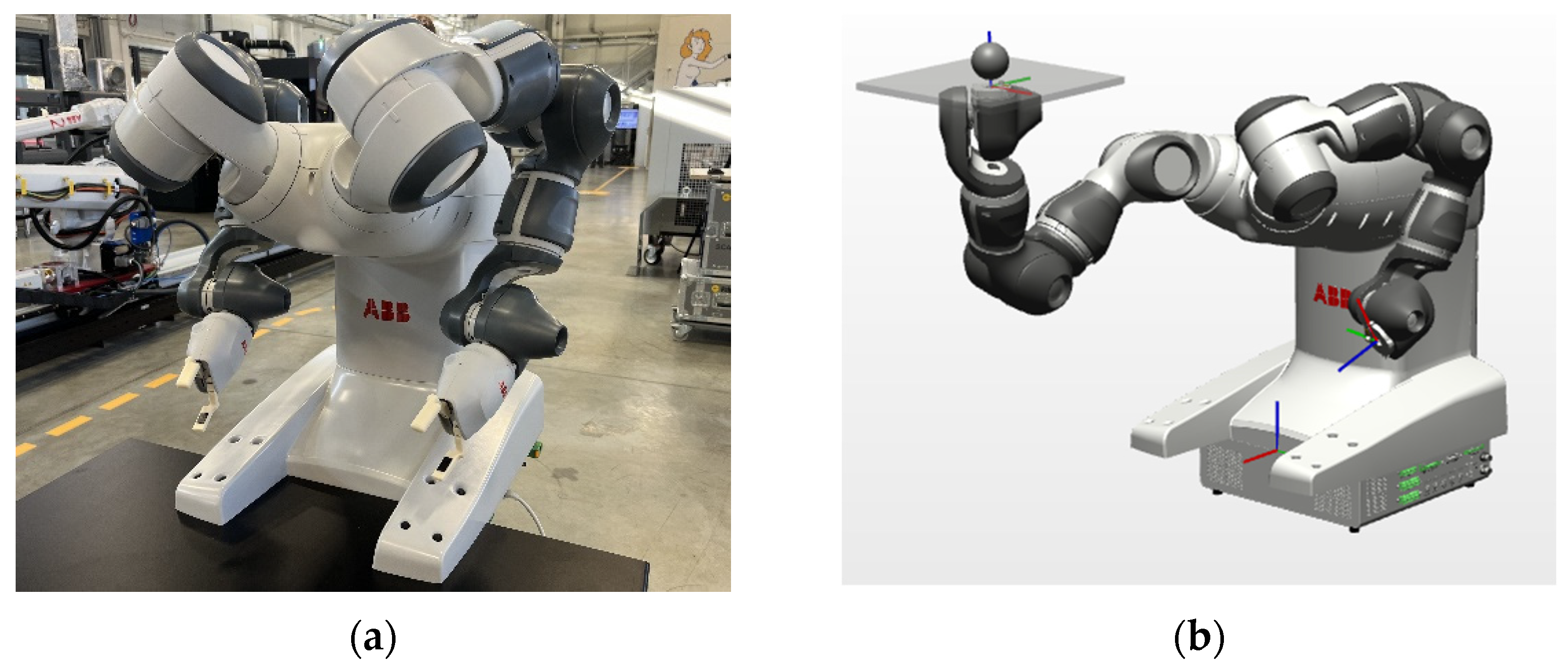
The robotic manipulator with 7 degrees of freedom (DoF) is chosen as the motion system of the Ball and Plate setup. It is a dual-arm collaborative robot, ABB IRB 14,000, shown in
Figure 3a. Only one manipulator arm of the robot is used for this paper, but it is possible to duplicate the solution for the second arm in the future, which can extend the plate to make it longer and be controlled by both arms in coordinated 14-DoF motion. The configuration of the manipulator, in which the plate is held, is shown in the simulation view in
Figure 3b.
There are two options for controlling the manipulator that are directly supported by the manufacturer and are non-invasive:
Standard point-to-point approach used for most applications of robotic manipulators, in which the manipulator plans its movements and executes them accordingly;
A direct method that bypasses the motion planner of the robot and executes the desired action directly without the path planning functionality (option EGM in ABB robots).
Both of these options for control are implemented and compared. The first option is expected to be much slower and may not be enough for such a fast, unstable system.
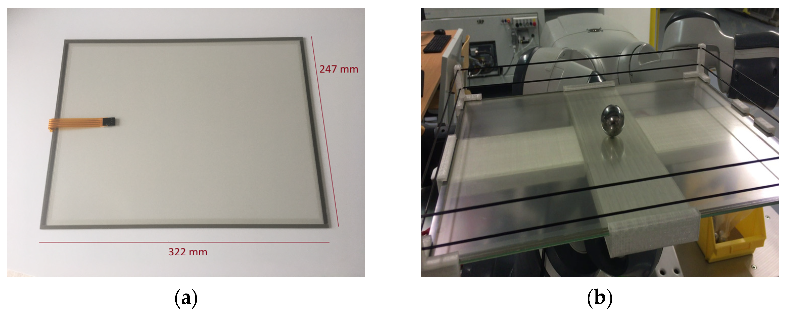
The sensor for the position of the ball is a resistive touchscreen glass commonly used in monitors with resistive touchscreens. It is an analog four-wire sensor that can be used instead of a more standard camera solution, which is prone to lightning conditions, reflections, and necessary calibration, and whose field of detection (view) cannot be covered by objects or hands. It is shown in
Figure 4 with its dimensions and mounted on the real robot.
5. Results
The results of the Ball and Plate system controlled by a 7-DoF collaborative robot manipulator are presented in this chapter, starting with the identification of parameters of the whole system and calculating controller parameters based on these findings. These results show the quality of the designed controller, its robustness against controller value disturbances, and its ability to stabilize the desired system.
5.1. System Identification
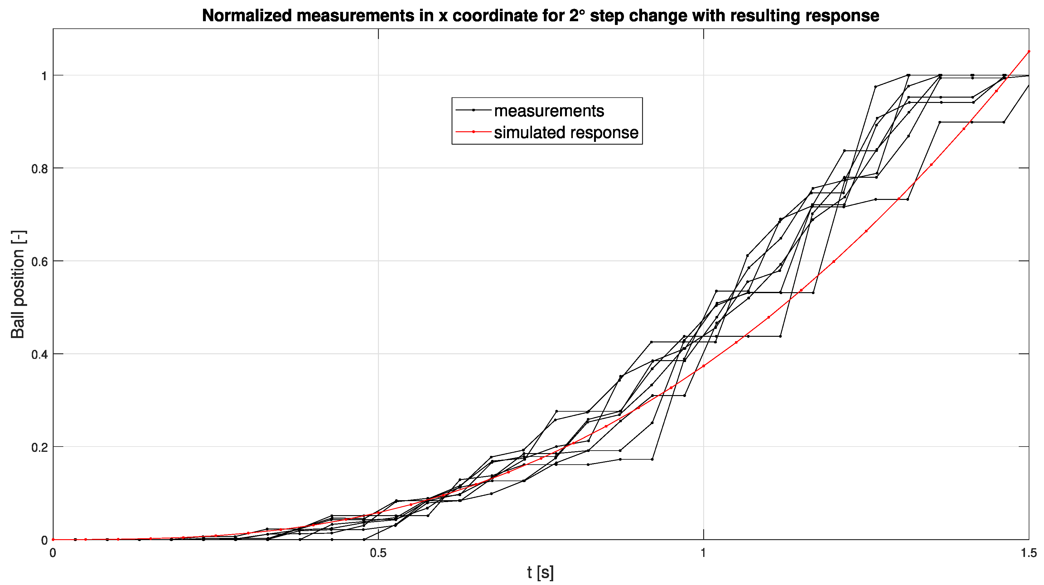
The dynamic parameters of the manipulator are not disclosed by the manufacturer, and the manipulator is handling its own kinematic and dynamic calculations, so identification of the whole system is needed. Parameters of the system presented in Equation (5) are identified from measurements of a step response of the system, approximated by a least-square minimization method and the Nelder—Mead simplex algorithm. The step response is a solid choice in this case because of the unstable nature of the system, which could be unpredictably excited by a signal with more complicated characteristics. Careful choice of an excitation signal must be considered and step change is predictable enough to provide valid results while keeping the ball on the expected path. The configuration of the manipulator is the same as presented in
Figure 3b, which is also the configuration used for control, and the system is not symmetric for
x and
y coordinates, thus both must be identified separately, although results for only the
x-coordinate are presented below.
Figure 5 shows multiple-step responses for a 2-degree step change, but the resulting approximation is the result of multiple measurements and multiple step values in the range from −3 to 3 degrees. The same procedure was taken in the simulation environment of RobotStudio, which provides precise virtualization of the robot, and the results of this pseudo-identification were analyzed in the same way as the real results presented in this paper.
The system approximated from these measurements is based on the structure of Equation (5) and, for this specific case, has the following result for both
x and
y coordinates:
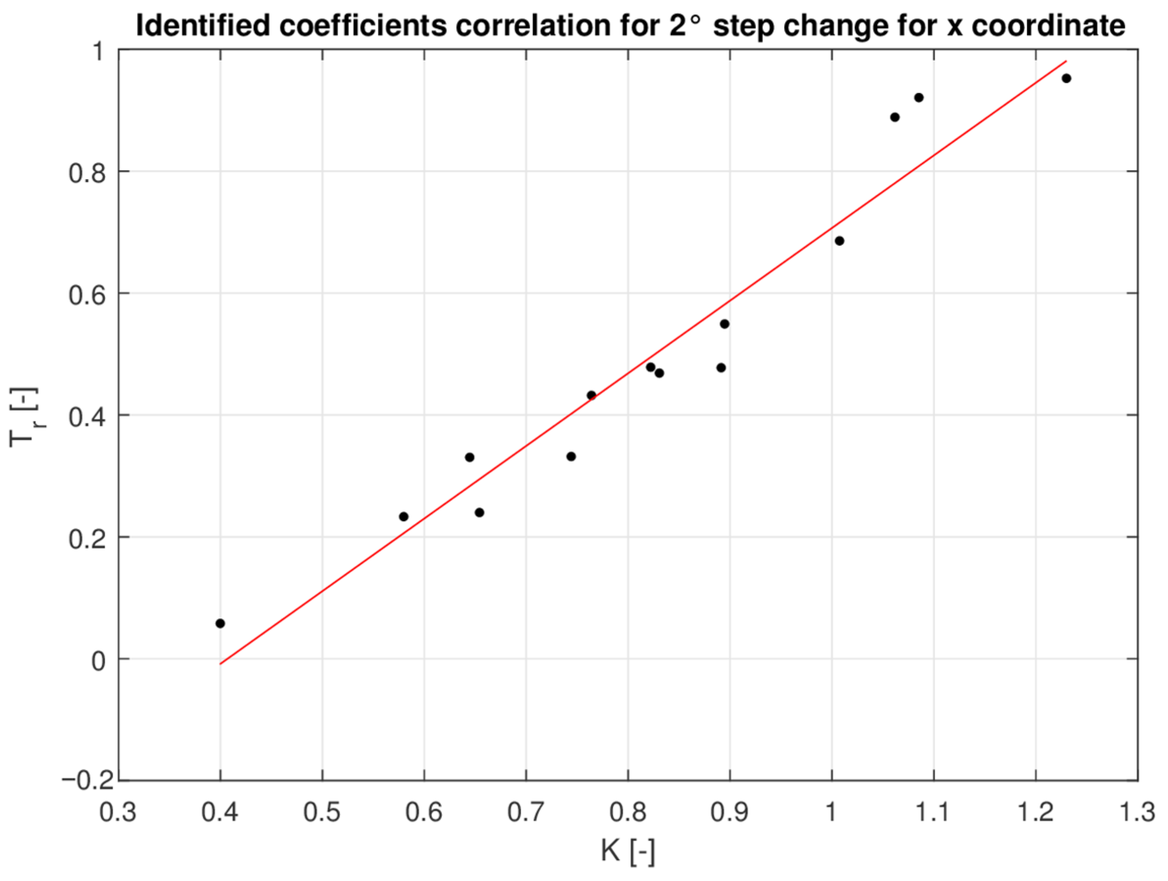
The correlation of identified parameters is also presented in
Figure 6, showing how closely related coefficients of unstable aperiodic systems are and how different combinations of values provide similar responses.
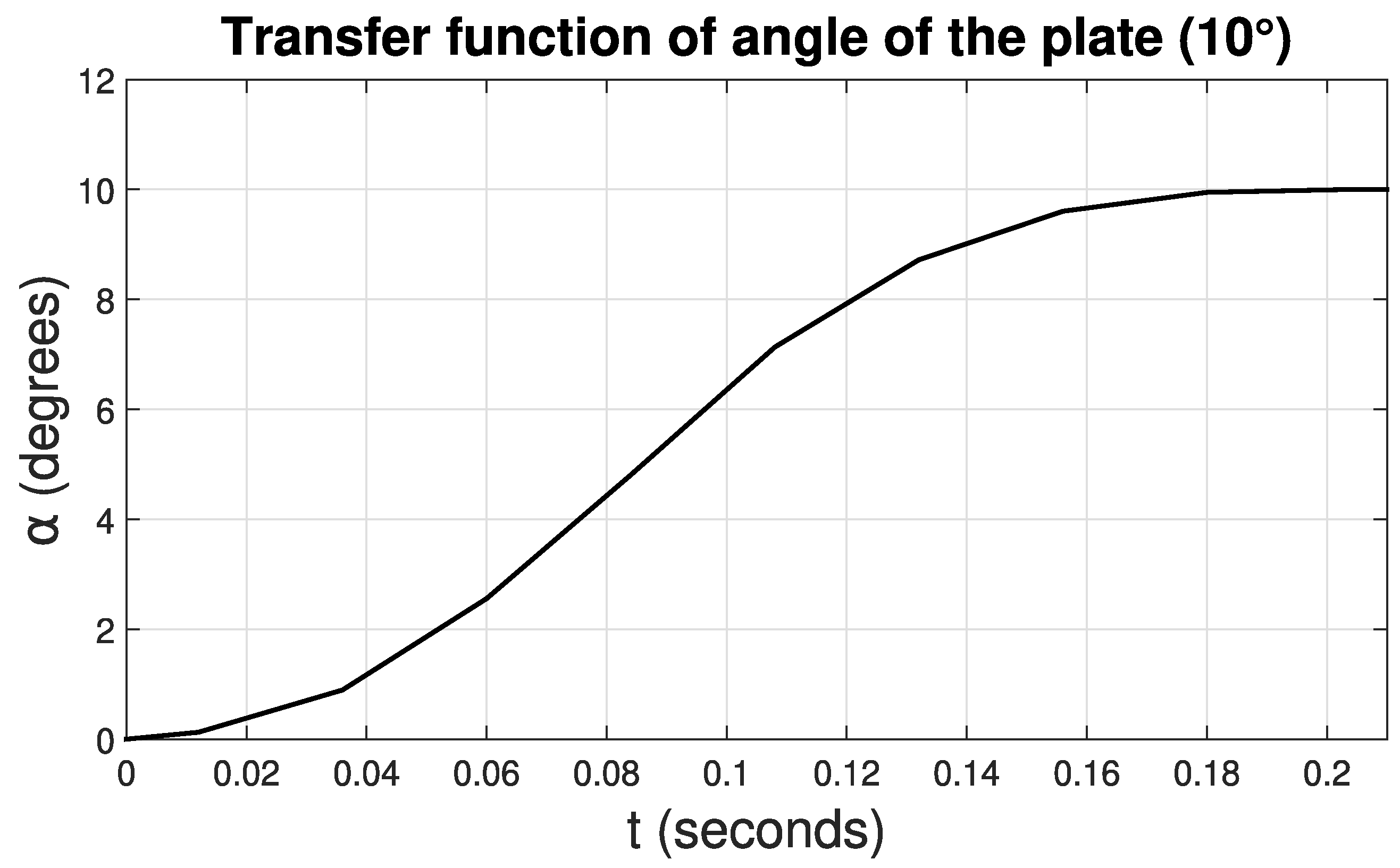
The transfer function of the manipulator was also measured to correctly estimate the sampling period and see how good the estimation of a 1st-order system’s dynamics is in Equation (5).
Figure 7 shows this measurement, and it can be seen that it has 2nd-order dynamics. The first control tests were conducted with an approximation of the 2nd-order system, but it had no benefit in results, so a 1st-order system approximation was used to simplify calculations.
5.2. Controller Designs and Parameters
The identified system was discretized with a sampling period of 0.05 s. It is based on the dynamics of the manipulator from
Figure 7, which showed it can reach a 2-degree angle in this time, which is enough for most of the movements needed for control. This discretized system, expressed in the Z-transform, has the following structure and parameters:
As stated in previous chapters, the optimal solution provides only half of the needed poles of the characteristic polynomial, so the other half must be chosen. The remaining three poles are all chosen to be real and to have the same value,
pp1,2,3 = 0.92. This creates half of the characteristic polynomial
D(
z−1):
The other half is calculated numerically using the Polynomial Toolbox with a penalization constant,
qu = 10, and for each coordinate, it leads to:
The resulting characteristic polynomials for
x and
y coordinates (
Dx(
z−1) and
Dy(
z−1)) are thus a product of the pole-placed part and the calculated part using spectral factorization:
Solving the Diophantine equations by comparing the coefficients of the
z−i characteristic polynomial in Equation (9) leads to the solution of the controller coefficients:
These parameters were implemented according to Equation (12) and are shown below in matrix form:
5.3. Real System Control
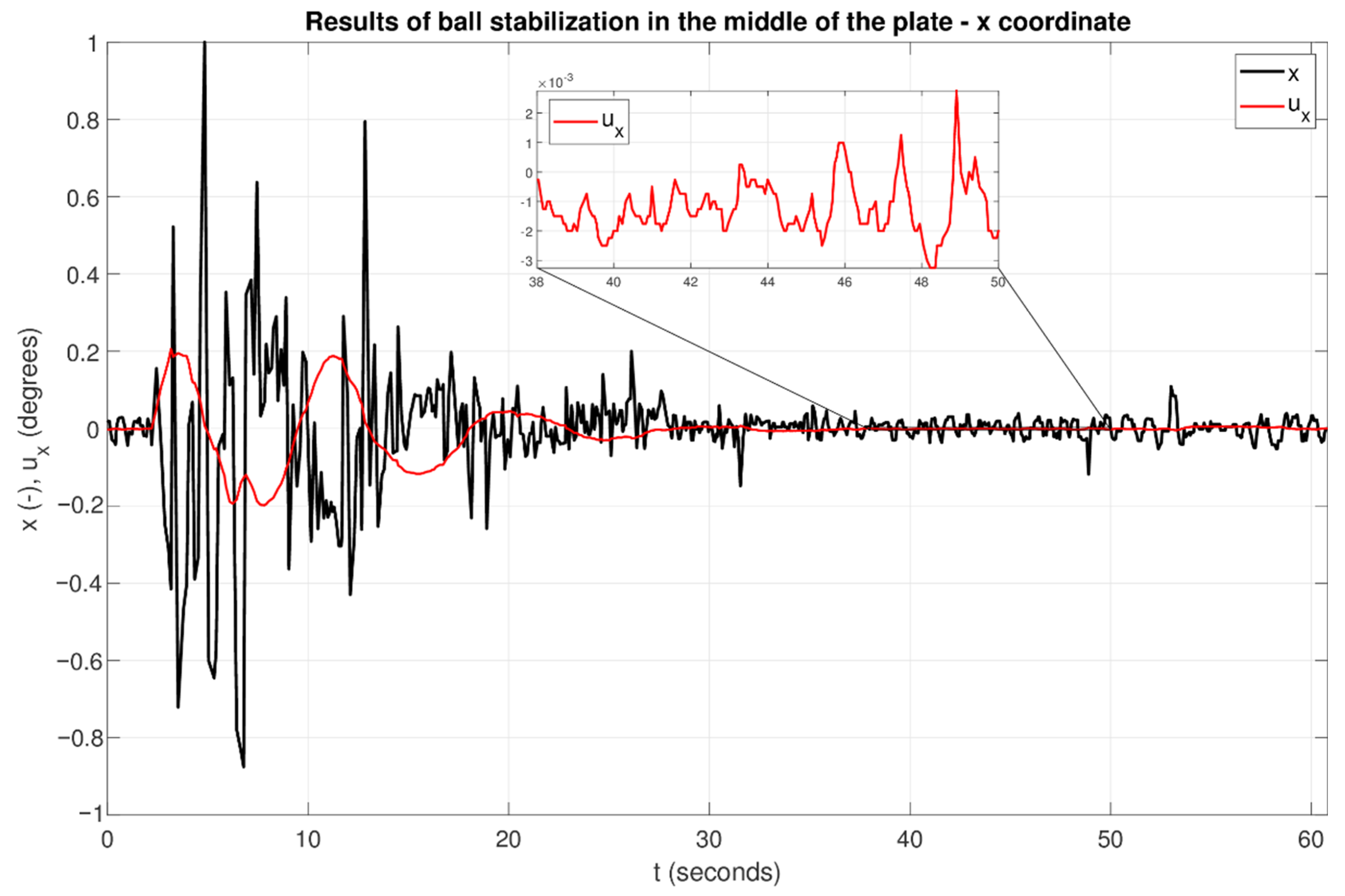
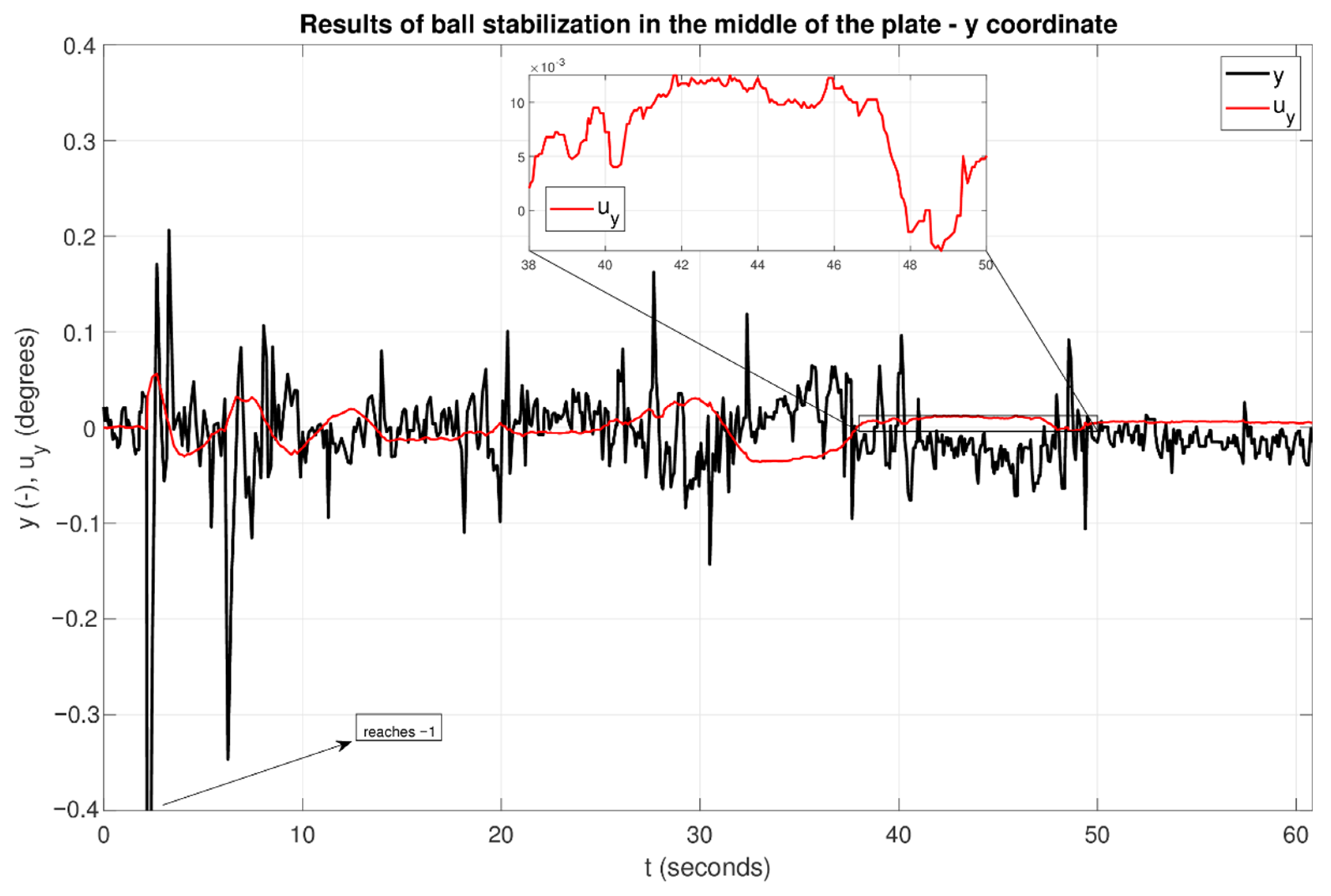
The first implementation of the robot system was by using its motion planner to plan movements controlled by the designed controller. The reference value was in the middle of the plate (0 for both coordinates), thus only stabilization was tested in this case. In the beginning, a disturbance was introduced to the position of the ball in the form of a force with random magnitude and direction.
Figure 8 and
Figure 9 show this control process. Using a motion planner is not the best strategy. It executes approximately every sixth command from the controller (not displayed in the figures) and hardly keeps the system stable. Figures show the system was able to stabilize the ball around the center in approximately 30 s, after which it was still not completely stabilized with expected angles of zero (the only values at the edge of stability). Figures thus show a closeup of the angle to show there is still an error and that the controller is trying to compensate for it, although very slightly in the magnitude of thousands of degrees. It can be best seen in the
x-coordinate results.
This bad quality of control is obvious when not every calculated action value is executed or is executed with a large time delay compared to the dynamics of the process. This big bottleneck is caused by the robot’s system execution policy, which is advantageous in standard point-to-point applications but not well handled for fast processes.
It is worth mentioning how robust the controller is, given that it stabilizes the system in these conditions despite the poor control quality and slow settle time. Such a large disturbance as skipping the controller’s output value is a tough task to handle, and the designed controller is at least keeping the system stable.
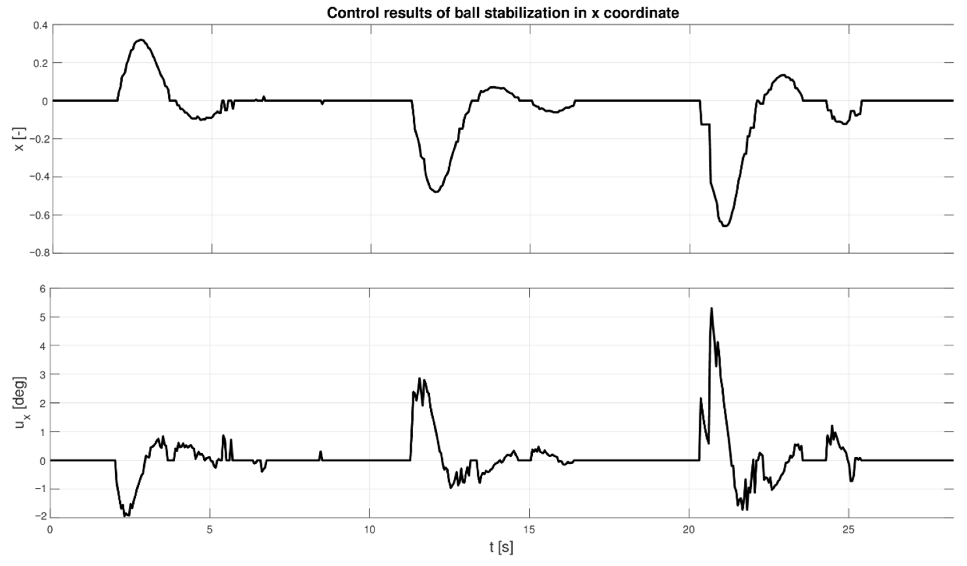
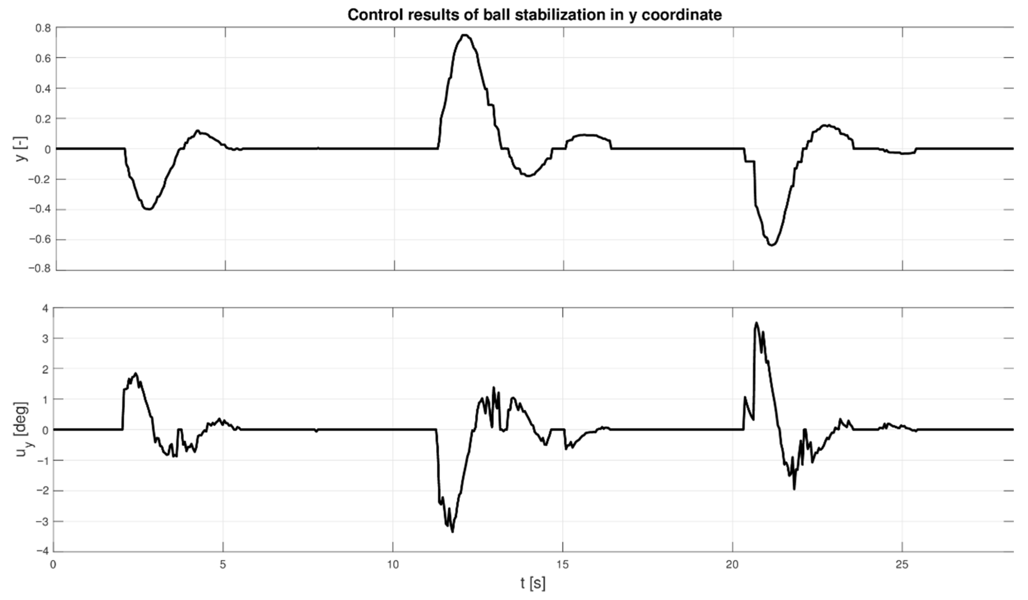
Another approach was bypassing the motion planner of the robot and sending commands from the controller directly to the motion system, using the option of the robot controller called EGM (Externally Guided Motion). This approach can send commands to the robot with a latency of 4–20 ms, which is still below the 0.05 s sampling period used in the controller design. Multiple disturbances were injected during measurements, always a few seconds after the ball was stabilized in the center. These measurements are presented in
Figure 10 and
Figure 11.
These disturbances can be seen at times of 2, 12, and 20 s, approximately. The force applied to the ball was gradually increased, and the ball deviated to, , and of the dimension of the plate in the x direction. The rate of change of the angle is quite large, and the angle reaches five degrees in the last case, which could be damped a little by choosing a larger qu value in the controller calculation or by placing three poles closer to one. However, this would make the control action slower and the settling time longer. It can be seen that the ball is stabilized in approximately 5 s for each magnitude of disturbance, which is relatively good and constant behavior with just a minor overshoot on the way back to the center.
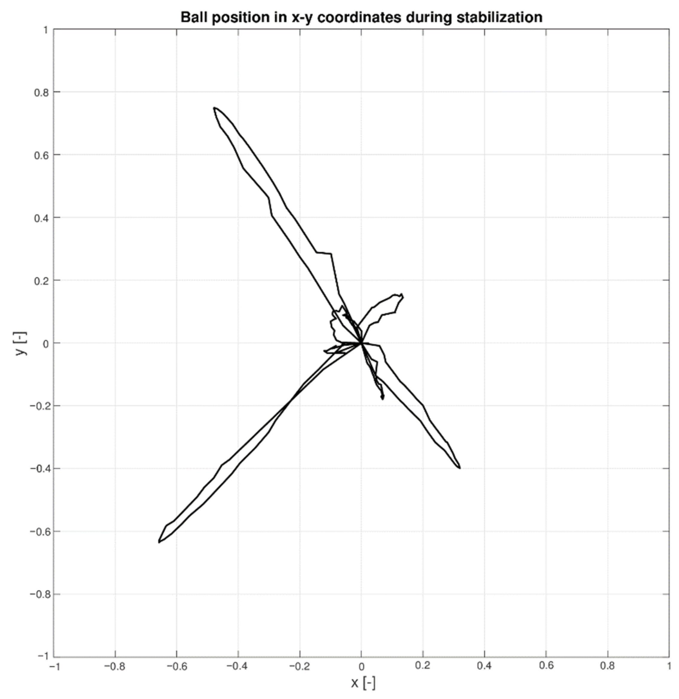
Figure 12 shows the position of the ball in the x-y plane, and both coordinates are displayed together, omitting the time axis. The direction of external disturbances is visible there, intentionally each in a different direction so they do not overlap in the x-y plot. It does not show how quickly the ball returns to the center, but rather the path it takes. The ball starts in the center and returns thereafter each disturbance is applied, and the plot thus shows mainly the movement of the ball on the plate and its deflection from the center after each disturbance.
Figure 12 is directly related to
Figure 10 and
Figure 11 and omits the time axis in favor of presenting both
x and
y coordinates in one plot.
These results show that the designed controller is more than capable of stabilizing the system using a robotic manipulator while keeping the rate of change of plate angles at reasonable values regarding the robot’s mechanics and expected prolonged use. Robots are designed to repeat their tasks, so their actions cannot be brought to their maximum, and their service life needs to be kept in mind during the design of their movements.
6. Discussion
This paper presented the Ball and Plate problem and its solution using a collaborative robotic manipulator as an electro-mechanical part of the model. It also presented the design and usage of a 2-DoF LQ polynomial controller, in which spectral factorization of polynomials was explored in search of a more optimal solution compensating for the dynamics of the controlled system while keeping the controller effort (and its fast change) within the limits of the manipulator used. Before the experimental part was tested on a real manipulator, it was implemented in a simulation environment to verify the proposed methods and approaches. This feasibility study was then confidently implemented in the real system and thoroughly tested for ball stabilization and disturbance rejection. Results can provide a solid ground for education in automation courses, which are heavily influenced by robots and industrial robotic manipulators. The path to the solution leads through many disciplines and shows not only controller design strategies but also controller-robot operation and communication, the kinematics and dynamics of the robot, and the real application of the problem with its specific limitations and rules of operation.
Integrating the Ball and Plate model on a collaborative 7-axis manipulator is not the most optimal method of solving this problem, but the main purpose of this thesis was the usage of robotic manipulators and systems for fast and unstable processes, and the B&P model is the best representative of such a system to be used in laboratory conditions (together with an inverted pendulum). Applications of bipedal robots can greatly benefit from the algorithms proposed in this thesis, as these robots have to solve movement in space while stabilizing their own bodies, battery packs, and, more importantly, random external forces acting on them. These applications have been around for several decades, but the movement of bipedal robots was mostly reliant on shifting the weight from one leg to another, thus greatly reducing the unstable characteristics of the movement itself. Another very important feature of these robots used in real-world applications is the load on their actuators, gears, and other mechanical parts. Many controllers fail to maintain the correct ratio of fast stabilization and low controller effort. In addition, lower controller effort also reduces power consumption of the whole system, thus reducing operating costs and increasing the operation time of the robots running on batteries. Thus, the results shown in this thesis comply with the described criteria and reliably compete with standard algorithms used in control theory.
Author Contributions
Conceptualization, L.S. and J.V.; methodology, L.S.; software, L.S.; validation, J.V. and F.G.; formal analysis, J.V.; investigation, L.S.; resources, F.G.; data curation, L.S.; writing—original draft preparation, L.S.; writing—review and editing, J.V.; visualization, L.S.; supervision, F.G.; project administration, F.G.; funding acquisition, F.G. All authors have read and agreed to the published version of the manuscript.
Funding
This research received no external funding.
Informed Consent Statement
Not applicable.
Data Availability Statement
Not applicable.
Conflicts of Interest
The authors declare no conflict of interest.
References
- An, C.H.; Atkeson, C.; Hollerbach, J. Model-Based Control of a Robot Manipulator; MIT Press: Cambridge, MA, USA, 1988. [Google Scholar]
- Hsia, T.C.; Gao, L.S. Robot manipulator control using decentralized linear time-invariant time-delayed joint controllers. In Proceedings of the IEEE International Conference on Robotics and Automation, Cincinnati, OH, USA, 13–18 May 1990; pp. 22–23. [Google Scholar]
- Lewis, F.; Dawson, D.; Abdallah, C. Robot Manipulator Control: Theory and Practice, 2nd ed.; Marcel Dekker: New York, NY, USA, 2004. [Google Scholar]
- Kelly, R.; Santibanez, V.; Loria, A. Control of Robot Manipulators in Joint Space; Springer: London, UK, 2005. [Google Scholar]
- Khan, M.F.; Islam, R.; Iqbal, J. Control strategies for robotic manipulators. In Proceedings of the 2012 International Conference of Robotics and Artificial Intelligence, Rawalpindi, Pakistan, 22–23 October 2012. [Google Scholar]
- Lee, J.; Chang, P.H.; Jin, M. Adaptive Integral Sliding Mode Control with Time-Delay Estimation for Robot Manipulators. IEEE Trans. Ind. Electron. 2017, 64, 6796–6804. [Google Scholar] [CrossRef]
- Khatib, O.; Burdick, J. Motion and force control of robot manipulators. In Proceedings of the1986 IEEE International Conference on Robotics and Automation, San Francisco, CA, USA, 7–10 April 1986. [Google Scholar]
- Zeng, G.; Hemami, A. An overview of robot force control. In Robotica; Cambridge University Press: Cambridge, UK, 1997; Volume 15, pp. 473–482. [Google Scholar]
- Basanez, L.; Rosell, J. Robotic polishing systems. IEEE Robot. Autom. Mag. 2005, 12, 35–43. [Google Scholar] [CrossRef]
- Perrusquia, A.; Yu, W.; Soria, A. Position/force control of robot manipulators using reinforcement learning. Ind. Robot 2019, 46, 267–280. [Google Scholar] [CrossRef]
- Mishra, A.K.; Meruvia-Pastor, O. Robot arm manipulation using depth-sensing cameras and inverse kinematics. In Proceedings of the 2014 Oceans-St. John’s, St. John’s, NL, Canada, 14–19 September 2014. [Google Scholar]
- Behzadi-Khormouji, H.; Derhami, V.; Rezaeian, M. Adaptive Visual Servoing Control of robot Manipulator for Trajectory Tracking tasks in 3D Space. In Proceedings of the 2017 5th RSI International Conference on Robotics and Mechatronics (ICRoM), Tehran, Iran, 25–27 October 2017. [Google Scholar]
- Neto, P.; Pires, J.N.; Moreira, A.P. Accelerometer-based control of an industrial robotic arm. In Proceedings of the 18th IEEE International Symposium on Robot and Human Interactive Communication, Toyama, Japan, 27 September–2 October 2009. [Google Scholar]
- Murillo, P.C.U.; Moreno, R.J.; Sanchez, O.F.A. Individual Robotic Arms Manipulator Control Employing Electromyographic Signals Acquired by Myo Armbands. Int. J. Appl. Eng. Res. 2016, 11, 11241–11249. [Google Scholar]
- Gracia, L.; Solanes, J.E.; Munoz-Benavent, P.; Miro, J.V. Human-robot collaboration for surface treatment tasks. Interact. Stud. 2019, 20, 148–184. [Google Scholar] [CrossRef]
- Kebria, P.M.; Khosravi, A.; Nahavandi, S.; Shi, P.; Alizadehsani, R. Robust Adaptive Control Scheme for Teleoperation Systems With Delay and Uncertainties. IEEE Trans. Cybern. 2019, 50, 3243–3253. [Google Scholar] [CrossRef] [PubMed]
- Girbes-Juan, V.; Schettino, V.; Demiris, Y.; Tornero, J. Haptic and Visual Feedback Assistance for Dual-Arm Robot Teleoperation in Surface Conditioning Tasks. IEEE Trans. Haptics 2020, 14, 44–56. [Google Scholar] [CrossRef] [PubMed]
- Gonzalez, C.; Solanes, J.E.; Munoz, A.; Gracia, L. Advanced teleoperation and control system for industrial robots based on augmented virtuality and haptic feedback. J. Manuf. Syst. 2021, 59, 283–298. [Google Scholar] [CrossRef]
- Stone, K.A.; Dittrich, S.; Luna, M.; Heidari, O.; Perez-Gracia, A.; Schoen, M. Augmented reality interface for industrial robot controllers. In Proceedings of the 2020 Intermountain Engineering, Technology and Computing (IETC), Orem, UT, USA, 2–3 October 2020. [Google Scholar]
- Yoshikawa, T.; Sudou, A. Dynamic hybrid position/force control of robot manipulators-on-line estimation of unknown constraint. IEEE Trans. Robot. Autom. 1993, 9, 220–226. [Google Scholar] [CrossRef]
- Bjerkeng, M.; Transeth, A.A.; Pettersen, K.Y.; Kyrkjebo, E.; Fjerdingen, S.A. Active camera control with obstacle avoidance for remote operations with industrial manipulators: Implementation and experimental results. In Proceedings of the 2011 IEEE/RSJ International Conference on Intelligent Robots and Systems, San Francisco, CA, USA, 25–30 September 2011. [Google Scholar]
- Dzedzickis, A.; Subačiūtė-Žemaitienė, J.; Šutinys, E.; Samukaitė-Bubnienė, U.; Bučinskas, V. Advanced Applications of Industrial Robotics: New Trends and Possibilities. Appl. Sci. 2022, 12, 135. [Google Scholar] [CrossRef]
- Bruce, J.; Keeling, C.; Rodriguez, R. Four Degree of Freedom Control System Using a Ball on a Plate. Master’s Thesis, Southern Polytechnic State University, Marietta, GA, USA, 2011. [Google Scholar]
- Stander, D.; Jimenez-Leudo, S.; Quijano, N. Low-Cost “ball and Plate” design and implementation for learning control systems. In Proceedings of the 2017 IEEE 3rd Colombian Conference on Automatic Control (CCAC), Cartagena, Colombia, 18–20 October 2017. [Google Scholar]
- Jadlovska, A.; Jajcisin, S.; Lonscak, R. Modelling and PID Control Design of Nonlinear Educational Model Ball & Plate. In Proceedings of the 17th International Conference on Process Control ‘09, Strbske Pleso, Slovakia, 9–12 June 2009. [Google Scholar]
- Awtar, S.; Bernard, C.; Boklund, N.; Master, A.; Ueda, D.; Craig, K. Mechatronic design of a ball-on-plate balancing system. Mechatronics 2002, 12, 217–228. [Google Scholar] [CrossRef]
- Kassem, A.; Haddad, H.; Albitar, C. Commparison Between Different Methods of Control of Ball and Plate System with 6DOF Stewart Platform. IFAC-Pap. 2015, 48, 47–52. [Google Scholar] [CrossRef]
- Koszewnik, A.; Troc, K.; Slowik, M. PID Controllers Design Applied to Positioning of Ball on the Stewart Platform. Acta Mech. Et Autom. 2014, 8, 214–218. [Google Scholar] [CrossRef]
- Khan, K.A.; Konda, R.; Ryu, J.-C. ROS-based control for a robot manipulator with a demonstration of the ball-on-plate task. Adv. Robot. Res. 2018, 2, 113–127. [Google Scholar]
- Lee, K.-K.; Batz, G.; Wollherr, D. Basketball robot: Ball-On-Plate with pure haptic information. In Proceedings of the 2008 IEEE International Conference on Robotics and Automation, Pasadena, CA, USA, 19–23 May 2008. [Google Scholar]
- Shih, C.-L.; Hsu, J.-H.; Chang, C.-J. Visual Feedback Balance Control of a Robot Manipulator and Ball-Beam System. J. Comput. Commun. 2017, 5, 8–18. [Google Scholar] [CrossRef][Green Version]
- Wang, H.; Tian, Y.; Sui, Z.; Zhang, X.; Ding, C. Tracking Control of Ball and Plate System with a Double Feedback Loop Structure. In Proceedings of the 2007 International Conference on Mechatronics and Automation, Harbin, China, 5–8 August 2007. [Google Scholar]
- Moarref, M.; Saadat, M.; Vossoughi, G. Mechatronic design and position control of a novel ball and plate system. In Proceedings of the 2008 16th Mediterranean Conference on Control and Automation, Ajaccio, France, 25–27 June 2008. [Google Scholar]
- Tian, Y.; Bai, M.; Su, J. A non-linear switching controller for ball and plate system. Int. J. Model. Identif. Control 2006, 1, 177–182. [Google Scholar] [CrossRef]
- Ghiasi, A.; Jafari, H. Optimal Robust Controller Design for the Ball and Plate System. In Proceedings of the 9th International Conference on Electronics Computer and Computation ICECCO-2012, Ankara, Turkey, 1–3 November 2012. [Google Scholar]
- Bobal, V.; Bohm, J.; Fessl, J.; Machacek, J. Digital Self-Tuning Controllers; Springer: London, UK, 2005. [Google Scholar]
- PolyX-The Polynomial Toolbox for Use with MATLAB. Available online: http://www.polyx.com (accessed on 28 October 2022).
- YuMi®-IRB 14000|Collaborative Robot. Available online: https://new.abb.com/products/robotics/collaborative-robots/yumi/irb-14000-yumi (accessed on 18 December 2020).
| Publisher’s Note: MDPI stays neutral with regard to jurisdictional claims in published maps and institutional affiliations. |
© 2022 by the authors. Licensee MDPI, Basel, Switzerland. This article is an open access article distributed under the terms and conditions of the Creative Commons Attribution (CC BY) license (https://creativecommons.org/licenses/by/4.0/).


