A Four Step Feedback Iteration and Its Applications in Fractals

Abstract

Fractals play a vital role in modeling the natural environment. The present aim is to investigate the escape criterion to generate specific fractals such as Julia sets, Mandelbrot sets and Multi-corns via F-iteration using complex functions $h\left(z\right)=z^n+c$, $h\left(z\right)=sin\left(z^n\right)+c$ and $h\left(z\right)=e^{z^n}+c$, $n\ge 2,c\in \mathbb{C}$. We observed some beautiful Julia sets, Mandelbrot sets and Multi-corns for n = 2, 3 and 4. We generalize the algorithms of the Julia set and Mandelbrot set to visualize some Julia sets, Mandelbrot sets and Multi-corns. Moreover, we calculate image generation time in seconds at different values of input parameters.

1. Introduction

Fractals occur frequently in the natural environment and their role is vital to measure the optimization of energy, quantification of ${CO}_2$, enhancement of the range of antennas, and performance of the stock market and musical compositions due to their natural fractal patterns. Such patterns can be generated by using various iterative algorithms in computers. This approach can be successfully applied in various fields to create future technologies by ensuring secure development (https://fractal-project.eu/) and fixed point theory plays a very vital role in the fractal theory for fractal generation via escape time criteria. Initially, the fractal was sketched by Benoit Mandelbrot, who is known as the father of fractal geometry, extending the work of Gaston Julia [1] who started this work in 1918 and successfully approximated the complex function $z⟶z^2+b$—where z, b$\in \mathbb{C}$—but was unable to sketch it. Mandelbrot [2] drew the graph of $z⟶z^2+b$, where $z,b\in \mathbb{C}$, in 1983 and, by changing the role of z and b in J-set, defined a new set known as M-set. J-set elaborates the role of iterates for every z and M-set explains the connected J-set for each b by elaborating those sets. M-set using $h:z\to z^p+c$, where $p\ge 2$, is explained in [3]. Later on, anti-fractals were defined by Crow et al. [4] for ${\overline{z}}^2+c$, which are tricorns.

Researchers use fixed point iterative schemes to generate fractals. Higher dimensional fractals are discussed in [5,6]. Generalized Julia sets and Mandelbrot sets are generated by using different iterative schemes such as Mann iteration [7], Ishikawa iteration [8], S-iteration [9], Noor iteration [10], SP-iteration [11] and CR-iteration [12]. Fractals via modified Jungck-S orbit are discussed in [13]. M-set and J-sets by Jungck type scheme with s-convexity are elaborated in [14]. Fractals such as filled J-set by Jungck Mann scheme are discussed in [15]. Fractals via extended Jungck-SP orbit are discussed in [16]. Further, we can find biomorphs in literature, which are generated by different iterations [17,18,19]. J-set and M-set for complex trigonometric function via different iterations are discussed in [20]. Hybrid Picard–Mann iteration has been used to generate anti-fractals [21]. In this article, we use F-iteration [22] to generate the Julia set, Mandelbrot set and Multi-corns for the Complex function $h\left(z\right)=z^n+c$, where $n\ge 2,c\in \mathbb{C}$.

2. Preliminaries

In this part of the paper, we study some well-known fractals and iterative algorithms.

Definition 1. 

([1]). Assume that $F_h$ is the set of points in $\mathbb{C}$ such that $h:\mathbb{C}\to \mathbb{C}$ is a complex polynomial of degree $\ge 2$. The set $F_h$ is called a filled Julia set when the orbit of $F_h\nrightarrow \infty$ as $i\to \infty$, i.e.,

$$F_h=\{z\in \mathbb{C}:\{|h^i\left(z\right)\left|\right\}{}_{i=0}^{\infty }isbounded\}.$$

(1)

The set of boundary points of $F_h$ is known as a simple J-set.

Definition 2. 

([23]). A set consisting of all the connected J-sets is called a Mandelbrot set (M-set), i.e.,

$$M=\{c\in \mathbb{C}:F_{h}isconnected\},$$

(2)

correspondingly, we can define M-set as [24]

$$M=\{c\in \mathbb{C}:\left\{h^i\left(0\right)\right\}\nrightarrow \infty asi\to \infty \},$$

(3)

where 0 is the only critical point $\acute{h}\left(0\right)=0$. So, we choose 0 as the initial point.

Definition 3. 

(Multi-corn [23]). Let $h_b:\mathbb{C}\to \mathbb{C}$ be a mapping and $h_b\left(z\right)={\overline{z}}^n+b$ with $b\in \mathbb{C}$ being a parameter. Then, the multi-corn $J^{*}$ for $h_b$ is defined as the set of all $b\in \mathbb{C}$ for which the orbit of 0 under the mapping of $h_b$ is bounded, i.e.,

$$J^{*}=\{b\in \mathbb{C}:\left\{h{}_b^n\right\}\nrightarrow \infty \},$$

(4)

where $h{}_b^n$ is the $n^{th}$ iteration of function $h_b\left(z\right)$.

Definition 4. 

(Picard Iteration). Suppose that $h:\mathbb{C}\to \mathbb{C}$ is a complex function. Then, for any $z_0\in \mathbb{C}$, Picard’s iteration is given as

$$z_{k+1}=h\left(z_k\right),$$

(5)

where $k=0,1,2,\cdots$.

Definition 5. 

(Mann Iterative Process [25]). Assume that $h:\mathbb{C}\to \mathbb{C}$ is a complex mapping. For any $z_0\in \mathbb{C}$, Mann’s iterative scheme is given as

$$z_{k+1}=(1-\zeta )z_k+\zeta h\left(z_k\right),$$

(6)

where $\zeta \in (0,1]$ and $k=0,1,2,\cdots$.

Definition 6. 

(Ishikawa Iterative Process [26]). Let $h:\mathbb{C}\to \mathbb{C}$ be a mapping. For any $z_0\in \mathbb{C}$, the Ishikawa process is stated as

$$\left\{\begin{array}{c}{z}_{k+1}=(1-\alpha )z_k+\alpha h\left(y_k\right),\hfill \\ y_k=(1-\beta )z_k+\beta h\left(z_k\right),\hfill \end{array}\right.$$

(7)

where $\alpha ,\beta \in (0,1]$ and $k=0,1,2,\cdots$.

Definition 7. 

(F-iterative Scheme [22]). Assume that $h:\mathbb{C}⟶\mathbb{C}$ with $z_0\in \mathbb{C}$ is an initial guess; then, the F-iteration is

$$\left\{\begin{array}{c}{u}_k=(1-\alpha )z_k+\alpha h\left(z_k\right),\hfill \\ x_k=h\left(u_k\right),\hfill \\ y_k=h\left(x_k\right),\hfill \\ z_{k+1}=h\left(y_k\right),\hfill \end{array}\right.$$

(8)

where $\alpha \in (0,1]$ and $k=0,1,2,\cdots$

3. Main Results

In this section, we will prove some escape criteria for different functions via F-iteration.

Case I. 

(When $h_c\left(z\right)=z^n+c$.)

Theorem 1. 

Suppose that $h_c\left(z\right)=z^n+c$ with $n\ge 2$, $c\in \mathbb{C}$ is a complex polynomial with $\left|z\right|\ge \left|c\right|>2^{\frac{1}{n-1}}$ and $\left|z\right|>\left|c\right|>{\left(\frac{2}{\alpha }\right)}^{\frac{1}{n-1}}$. Further, suppose that $\left\{z_{k\in \mathbb{N}}\right\}$ is the sequence of iterates defined in (8); then, $|z_k|\to \infty$ as $i\to \infty .$

Proof. 

Since $h_c\left(z\right)=z^n+c$ and assuming that $z_0=z,u_0=u$, the initial step of F-iteration is

$$\begin{array}{c}|u_k|=|(1-\alpha )z_k+\alpha h\left(z_k\right)|.\hfill \end{array}$$

For $k=0$, we have

$$\begin{array}{c}\left|u\right|=\left|\right(1-\alpha )z+\alpha h(z\left)\right|\hfill \\ \left|u\right|=|(1-\alpha )z+\alpha (z^n+c)|\hfill \\ \left|u\right|\ge \alpha |z^n|-\alpha |c|-|z|+\alpha |z|\hfill \\ \left|u\right|\ge \alpha |z^n|-\alpha |z|-|z|+\alpha |z|\because \left|z\right|>\left|c\right|\hfill \\ \left|u\right|\ge \alpha |z^n|-|z|\hfill \\ \left|u\right|\ge \left|z\right|\left(\alpha |z^{n-1}|-1\right)\hfill \\ \left|u\right|\ge \left|z\right|.\because \left|z\right|>\left(\frac{2}{\alpha }\right)\hfill \end{array}$$

The second step of F-iteration is given as

$$\begin{array}{c}|x_k|=\left|h\right(u_k\left)\right|.\hfill \end{array}$$

For $i=0$, we have

$$\begin{array}{c}\left|x\right|=\left|h\right(u\left)\right|\hfill \\ \left|x\right|=|u^n+c|\hfill \\ \left|x\right|\ge |u^n|-|c|\hfill \\ \left|x\right|\ge |u^n|-|u|\hfill \\ \left|x\right|\ge \left|u\right|\left(|u^{n-1}-1\right)|\hfill \\ \left|x\right|\ge \left|u\right|\left|z\right|>2^{\frac{1}{n-1}}\hfill \end{array}$$

and the third step of F-iteration is

$$\begin{array}{c}|y_k|=\left|h\right(x_k\left)\right|.\hfill \end{array}$$

For $k=0$, we have

$$\begin{array}{c}\left|y\right|=\left|h\right(x\left)\right|\hfill \\ \left|y\right|=|x^n+c|\hfill \\ \left|y\right|\ge |x^n+c|\hfill \\ \left|y\right|\ge |x^n+c|\hfill \\ \left|y\right|\ge |x^n|-|x|\hfill \\ \left|y\right|\ge \left|x\right|\left(|x^{n-1}|-1\right)\hfill \end{array}$$

Since $\left|u\right|\ge \left|z\right|>2^{\frac{1}{n-1}}$, this implies that $|x^{n-1}|-1>1$; therefore,

$$\begin{array}{c}\left|y\right|\ge \left|x\right|.\hfill \end{array}$$

For the last step of F-iteration, we have

$$\begin{array}{c}|z_{k+1}|=\left|h\right(y_k\left)\right|.\hfill \end{array}$$

For $k=0$, we have

$$\begin{array}{c}|z_1|=\left|h\right(y\left)\right|\hfill \\ |z_1|=|y^n+c|\hfill \\ |z_1|\ge |y^n|-|c|\hfill \\ |z_1|\ge |z^n|-|z|\because \left|y\right|\ge \left|x\right|\ge \left|u\right|\ge \left|z\right|\ge \left|c\right|\hfill \\ |z_1|\ge \left|z\right|\left(z^{n-1}-1\right).\hfill \end{array}$$

For $k=1$,

$$\begin{array}{c}|z_2|\ge |z|{\left(z^{n-1}-1\right)}^2.\hfill \end{array}$$

Iterating up to the $k^{th}$ term, we have

$$\begin{array}{c}|z_3|\ge \left|z\right|{\left(z^{n-1}-1\right)}^3.\hfill \\ |z_4|\ge \left|z\right|{\left(z^{n-1}-1\right)}^4.\hfill \\ .\hfill \\ .\hfill \\ .\hfill \\ |z_k|\ge \left|z\right|{\left(z^{n-1}-1\right)}^k.\hfill \end{array}$$

Since $\left|z\right|>2^{\frac{1}{n-1}}⟹\left|z^{n-1}\right|-1>1$, $z_k\to \infty$ as $k\to \infty .$    □

Corollary 1. 

Consider that

$$\begin{array}{c}\left\{\begin{array}{c}{z}_m>max\left\{\left|b\right|,2^{\frac{1}{n-1}},{\left(\frac{2}{\alpha }\right)}^{\frac{1}{n-1}}\right\}\hfill \end{array}\right.\hfill \end{array}$$

for $m\ge 0$. Since $\left|z\right|>{\left(\frac{2}{\alpha }\right)}^{\frac{1}{n-1}}⟹\alpha \left|z^{n-1}\right|-1>1,$$|z_{m+k}|>|z\left|\right(\alpha |z^{n-1}{|-1)}^{m+k}$. Hence, $|z_k|\to \infty$ as $k\to \infty .$

Case II. 

(When $h_b\left(z\right)=sin\left(z^n\right)+b$.)

Let $h\left(z\right)=sin\left(z^n\right)+b$ with $n\ge 2,b\in \mathbb{C}$ be a sine function. Then, the Maclaurin expansion is

$$\begin{array}{cc}|sin(z^n\left)\right|\hfill & =\left|z^n-\frac{z^{3n}}{3!}+\frac{z^{5n}}{5!}-\frac{z^{7n}}{7!}+\cdots \right|\hfill \\ & \ge |z^n|\left|1-\frac{z^{2n}}{3!}+\frac{z^{4n}}{5!}-\frac{z^{6n}}{7!}+\cdots \right|\hfill \end{array}$$

Assume that

$$|{\eta }_4|\le \left|1-\frac{z^{2n}}{3!}+\frac{z^{4n}}{5!}-\frac{z^{6n}}{7!}+\cdots \right|$$

so, we have

$$\begin{array}{c}|sin(z^n\left)\right|\ge |{\eta }_4\left|\right|z^n|.\hfill \end{array}$$

Similarly,

$$\begin{array}{c}|sin(y^n\left)\right|\ge |{\eta }_3\left|\right|y^n|.\hfill \\ |sin(x^n\left)\right|\ge |{\eta }_2\left|\right|x^n|.\hfill \\ |sin(u^n\left)\right|\ge |{\eta }_1\left|\right|u^n|.\hfill \end{array}$$

Theorem 2. 

Suppose $h_b\left(z\right)=sin{\left(z\right)}^n+b$ with $n\ge 2$, $b\in \mathbb{C}$ is a trigonometric function with $\left|z\right|\ge \left|b\right|>{\left(\frac{2}{\alpha |{\eta }_4|}\right)}^{\frac{1}{n-1}}$,$\left|z\right|\ge \left|b\right|>{\left(\frac{2}{|{\eta }_1|}\right)}^{\frac{1}{n-1}}$,$\left|z\right|\ge \left|b\right|>{\left(\frac{2}{|{\eta }_2|}\right)}^{\frac{1}{n-1}}$ and $\left|z\right|\ge \left|b\right|>{\left(\frac{2}{|{\eta }_3|}\right)}^{\frac{1}{n-1}}$. Further, suppose that $\left\{z_{k\in \mathbb{N}}\right\}$ is the sequence of iterates defined in (8); then, $|z_k|\to \infty$ as $k\to \infty .$

Proof. 

As $h_b\left(z\right)=sin{\left(z\right)}^n+b$, the initial step of F-iterative process is given as

$$\begin{array}{c}|u_k|=|(1-\alpha )z_k+\alpha h\left(z_k\right)|.\hfill \end{array}$$

for $k=0$,

$$\begin{array}{c}|u_0|=|(1-\alpha )z_0+\alpha h\left(z_0\right)|\hfill \\ \left|u\right|=\left|\alpha h\right(z)+(1-\alpha \left)z\right|\hfill \\ \left|u\right|\ge \left|\alpha h\right(z\left)\right|-\left|\right(1-\alpha \left)z\right|\hfill \\ \left|u\right|\ge \alpha |sin\left(z^n\right)+b|-(1-\alpha )\left|z\right|\hfill \\ \left|u\right|\ge \alpha |z^n\left|\right|{\eta }_4|-\alpha |b|-(1-\alpha )|z|\hfill \\ \left|u\right|\ge \alpha |z^n\left|\right|{\eta }_4|-|z|\because \left|z\right|\ge \left|b\right|\hfill \\ \left|u\right|\ge \left|z\right|\left(\alpha \right|z^{n-1}\left|\right|{\eta }_4|-1)\hfill \\ \left|u\right|\ge \left|z\right|.\because \left|z\right|>{\left(\frac{2}{\alpha |{\eta }_4|}\right)}^{n-1}\hfill \end{array}$$

The second step of the F-iterative scheme is

$$\begin{array}{c}|x_k=h\left(u_k\right)|.\hfill \end{array}$$

for $k=0$,

$$\begin{array}{c}|x_0|=\left|h\right(u_0\left)\right|\hfill \\ \left|x\right|=|sin(u^n)+b|\hfill \\ \left|x\right|\ge |sin(u^n\left)\right|-\left|b\right|\hfill \\ \left|x\right|\ge |u^n\left|\right|{\eta }_1|-|b|\hfill \\ \left|x\right|\ge |u^n\left|\right|{\eta }_1|-|u|\because \left|u\right|\ge \left|z\right|\ge \left|b\right|\hfill \\ \left|x\right|\ge \left|u\right|\left(\right|u^{n-1}\left|\right|{\eta }_1|-1)\hfill \\ \left|x\right|\ge \left|u\right|\because \left|z\right|>{\left(\frac{2}{{\eta }_1}\right)}^{n-1}.\hfill \end{array}$$

The third step of F-iteration is

$$\begin{array}{c}|x_k|=\left|h\right(u_k\left)\right|\hfill \end{array}$$

for $k=0$,

$$\begin{array}{c}|y_0|=\left|h\right(x_0\left)\right|\hfill \\ \left|y\right|=|sin(x^n)+b|\hfill \\ \left|y\right|\ge |sin(x^n\left)\right|-\left|b\right|\hfill \\ \left|y\right|\ge |x^n\left|\right|{\eta }_2|-|b|\hfill \\ \left|y\right|\ge |x^n\left|\right|{\eta }_2|-|x|\because \left|z\right|\ge \left|b\right|\hfill \\ \left|y\right|\ge \left|x\right|\left(|x^{n-1}\left|\right|{\eta }_2|-1\right)\hfill \\ \left|y\right|\ge \left|x\right|.\because \left|z\right|>{\left(\frac{2}{{\eta }_2}\right)}^{n-1}\hfill \end{array}$$

The final step of F-iteration is as follows:

$$\begin{array}{c}|z_{k+1}|=\left|h\right(y_k\left)\right|\hfill \end{array}$$

for $k=0$,

$$\begin{array}{c}|z_1|=\left|h\right(y_0\left)\right|\hfill \\ |z_1|=|sin(y^n)+b|\hfill \\ |z_1|\ge |sin(y^n\left)\right|-\left|b\right|\hfill \\ |z_1|\ge |y^n\left|\right|{\eta }_3|-|b|\hfill \\ |z_1|\ge |z^n\left|\right|{\eta }_3|-|z|\because \left|z\right|\ge \left|b\right|\hfill \\ |z_1|\ge \left|z\right|\left(\right|z^{n-1}\left|\right|{\eta }_3|-1)\hfill \end{array}$$

Iterating this up to the $k^{th}$ terms,

$$\begin{array}{c}|z_2|\ge \left|z\right|\left(\right|z^{n-1}\left|\right|{\eta }_3{|-1)}^2\hfill \\ |z_3|\ge \left|z\right|\left(\right|z^{n-1}\left|\right|{\eta }_3{|-1)}^3\hfill \\ .\hfill \\ .\hfill \\ .\hfill \\ |z_k|\ge \left|z\right|\left(\right|z^{n-1}\left|\right|{\eta }_3{|-1)}^k\hfill \end{array}$$

Since $\left|z\right|>{\left(\frac{2}{{\eta }_3}\right)}^{\frac{1}{n-1}}⟹|{\eta }_3\left|\right|z^{n-1}|-1>1$, $z_k\to \infty$ as $k\to \infty .$    □

Corollary 2. 

Suppose

$$\begin{array}{c}\left\{\begin{array}{c}{z}_m>max\left\{\left|b\right|,{\left(\frac{2}{|{\eta }_1|}\right)}^{\frac{1}{n-1}},{\left(\frac{2}{|{\eta }_2|}\right)}^{\frac{1}{n-1}},{\left(\frac{2}{|{\eta }_3|}\right)}^{\frac{1}{n-1}},\left(\frac{2}{\alpha |{\eta }_4|}\right)\right\}\hfill \end{array}\right.\hfill \end{array}$$

for some $m\ge 0$. Since $\left|z\right|>{\left(\frac{2}{|{\eta }_1\left|\right|{\eta }_2\left|\right|{\eta }_3\left|\right|{\eta }_4|\alpha }\right)}^{\frac{1}{n-1}}⟹\left(|{\eta }_1\left|\right|{\eta }_2\left|\right|{\eta }_3\left|\right|{\eta }_4\left|\alpha \right|z^{n-1}|-1\right)>1,$$|z_{m+k}|>|z\left|\right(|{\eta }_1\left|\right|{\eta }_2\left|\right|{\eta }_3\left|\right|{\eta }_4\left|\alpha \right|z^{n-1}{|-1)}^{m+k}$. Hence, $|z_k|\to \infty$ as $k\to \infty .$

Case III. 

(When $h_b\left(z\right)=e^{z^n}+b$.)

Let $h_b\left(z\right)=e^{z^n}+b$ with $n\ge 2$, $b\in \mathbb{C}$ be a exponential function. Then, the Maclaurin expansion is

$$\begin{array}{cc}|e^{z^n}|\hfill & =\left|1+z^n+\frac{z^{2n}}{2!}+\frac{z^{3n}}{3!}+\frac{z^{4n}}{4!}+\cdots \right|\hfill \\ & \ge \left|z^n+\frac{z^{2n}}{2!}+\frac{z^{3n}}{3!}+\frac{z^{4n}}{4!}+\cdots \right|\hfill \\ & \ge |z^n|\left|1+\frac{z^n}{2!}+\frac{z^{2n}}{3!}+\frac{z^{3n}}{4!}+\cdots \right|.\hfill \end{array}$$

Assume that

$$|{\eta }_4|<\left|1+\frac{z^n}{2!}+\frac{z^{2n}}{3!}+\frac{z^{3n}}{4!}+\cdots \right|$$

so, we have

$$\begin{array}{c}|e^{z^n}|\ge |{\eta }_4\left|\right|z^n|.\hfill \end{array}$$

Similarly

$$\begin{array}{c}|e^{y^n}|\ge |{\eta }_3\left|\right|y^n|.\hfill \\ |e^{x^n}|\ge |{\eta }_2\left|\right|x^n|.\hfill \\ |e^{u^n}|\ge |{\eta }_1\left|\right|u^n|.\hfill \end{array}$$

Theorem 3. 

Suppose that $h_b\left(z\right)=e^{z^n}+b$ with $n\ge 2$, $b\in \mathbb{C}$ is a exponential function with $\left|z\right|\ge \left|b\right|>{\left(\frac{2}{\alpha |{\eta }_4|}\right)}^{\frac{1}{n-1}}$,$\left|z\right|\ge \left|b\right|>{\left(\frac{2}{|{\eta }_1|}\right)}^{\frac{1}{n-1}}$,$\left|z\right|\ge \left|b\right|>{\left(\frac{2}{|{\eta }_2|}\right)}^{\frac{1}{n-1}}$, $\left|z\right|\ge \left|b\right|>{\left(\frac{2}{|{\eta }_3|}\right)}^{\frac{1}{n-1}}$. Further, suppose that $\left\{z_{k\in \mathbb{N}}\right\}$ is the sequence of iterates defined in (8); then, $|z_k|\to \infty$ as $k\to \infty .$

Proof. 

As $h_b\left(z\right)=e^{z^n}+b$, the initial step of F-iteration is given as

$$\begin{array}{c}|u_k|=|(1-\alpha )z_k+\alpha h\left(z_k\right)|\hfill \end{array}$$

for $k=0$,

$$\begin{array}{c}|u_0|=|(1-\alpha )z_0+\alpha h\left(z_0\right)|\hfill \\ \left|u\right|=\left|\alpha h\right(z)+(1-\alpha \left)z\right|\hfill \\ \left|u\right|\ge \left|\alpha h\right(z\left)\right|-\left|\right(1-\alpha \left)z\right|\hfill \\ \left|u\right|\ge \alpha |e^{z^n}+b|-(1-\alpha )|z|\hfill \\ \left|u\right|\ge \alpha |z^n\left|\right|{\eta }_4|-\alpha |b|-(1-\alpha )|z|\hfill \\ \left|u\right|\ge \alpha |z^n\left|\right|{\eta }_4|-|z|\because \left|z\right|\ge \left|b\right|\hfill \\ \left|u\right|\ge \left|z\right|\left(\alpha \right|z^{n-1}\left|\right|{\eta }_4|-1)\hfill \\ \left|u\right|\ge \left|z\right|.\because \left|z\right|>{\left(\frac{2}{\alpha |{\eta }_4|}\right)}^{n-1}\hfill \end{array}$$

The second step of F-iteration is given as

$$\begin{array}{c}|x_k|=|h\left(u_k\right)|.\hfill \end{array}$$

for $k=0$,

$$\begin{array}{c}|x_0|=\left|h\right(u_0\left)\right|\hfill \\ \left|x\right|=|e^{u^n}+b|\hfill \\ \left|x\right|\ge |e^{u^n}|-|b|\hfill \\ \left|x\right|\ge |u^n\left|\right|{\eta }_1|-|b|\hfill \\ \left|x\right|\ge |u^n\left|\right|{\eta }_1|-|u|\because \left|z\right|\ge \left|b\right|\hfill \\ \left|x\right|\ge \left|u\right|\left(\right|u^{n-1}\left|\right|{\eta }_1|-1)\hfill \\ \left|x\right|\ge \left|u\right|\because \left|z\right|>{\left(\frac{2}{{\eta }_1}\right)}^{n-1}.\hfill \end{array}$$

The third step of F-iteration is

$$\begin{array}{c}|x_k|=\left|h\right(u_k\left)\right|\hfill \end{array}$$

for $k=0$,

$$\begin{array}{c}|y_0|=\left|h\right(x_0\left)\right|\hfill \\ \left|y\right|=|e^{x^n}+b|\hfill \\ \left|y\right|\ge |e^{x^n}|-|b|\hfill \\ \left|y\right|\ge |x^n\left|\right|{\eta }_2|-|b|\hfill \\ \left|y\right|\ge |x^n\left|\right|{\eta }_2|-|x|\because \left|z\right|\ge \left|b\right|\hfill \\ \left|y\right|\ge \left|x\right|\left(|x^{n-1}\left|\right|{\eta }_2|-1\right)\hfill \\ \left|y\right|\ge \left|x\right|.\because \left|z\right|>{\left(\frac{2}{{\eta }_2}\right)}^{n-1}\hfill \end{array}$$

The last step of F-iteration is as follows:

$$\begin{array}{c}|z_{k+1}||=|h\left(y_k\right)|\hfill \end{array}$$

for $k=0$,

$$\begin{array}{c}|z_1|=\left|h\right(y_0\left)\right|\hfill \\ |z_1|=|e^{y^n}+b|\hfill \\ |z_1|\ge |e^{y^n}|-|b|\hfill \\ |z_1|\ge |y^n\left|\right|{\eta }_3|-|b|\hfill \\ |z_1|\ge |z^n\left|\right|{\eta }_3|-|z|\because \left|z\right|>\left|b\right|\hfill \\ |z_1|\ge \left|z\right|\left(\right|z^{n-1}\left|\right|{\eta }_3|-1)\hfill \end{array}$$

Iterating this up to $k^{th}$ terms,

$$\begin{array}{c}|z_2|\ge \left|z\right|\left(\right|z^{n-1}\left|\right|{\eta }_3{|-1)}^2\hfill \\ |z_3|\ge \left|z\right|\left(\right|z^{n-1}\left|\right|{\eta }_3{|-1)}^3\hfill \\ .\hfill \\ .\hfill \\ .\hfill \\ |z_k|\ge \left|z\right|\left(\right|z^{n-1}\left|\right|{\eta }_3{|-1)}^k\hfill \end{array}$$

Since $\left|z\right|>{\left(\frac{2}{{\eta }_3}\right)}^{\frac{1}{n-1}}⟹|{\eta }_3\left|\right|z^{n-1}|-1>1$, $z_k\to \infty$ as $k\to \infty .$    □

Corollary 3. 

Consider

$$\begin{array}{c}\left\{\begin{array}{c}|z_m|>max\left\{\left|b\right|,{\left(\frac{2}{{\eta }_1}\right)}^{\frac{1}{n-1}},{\left(\frac{2}{{\eta }_2}\right)}^{\frac{1}{n-1}},{\left(\frac{2}{{\eta }_3}\right)}^{\frac{1}{n-1}},\left(\frac{2}{\alpha {\eta }_4}\right)\right\}\hfill \end{array}\right.\hfill \end{array}$$

for some $m\ge 0$. Since $\left|z\right|>{\left(\frac{2}{|{\eta }_1\left|\right|{\eta }_2\left|\right|{\eta }_3\left|\right|{\eta }_4|\alpha }\right)}^{\frac{1}{n-1}}⟹\left(|{\eta }_1\left|\right|{\eta }_2\left|\right|{\eta }_3\left|\right|{\eta }_4\left|\alpha \right|z^{n-1}|-1\right)>1,$$|z_{m+k}|>|z\left|\right(|{\eta }_1\left|\right|{\eta }_2\left|\right|{\eta }_3\left|\right|{\eta }_4\left|\alpha \right|z^{n-1}{|-1)}^{m+k}$. Hence, $|z_k|\to \infty$ as $k\to \infty .$

4. Applications

This section presents some anti-Julia sets via proposed iteration. To generate anti-Julia sets, a criteria to execute image is needed to run the algorithm. In the generation of fractals, some popular algorithms are used (i.e., Distance Estimator [27], Potential Function Algorithm [28] and escape criteria [29,30]).

In this paper, we use escape criteria in Algorithms 1–3 to generate the J-sets, M-sets and Multi-corns. The graphs are generated on an “Intel(R) Core(TM) i7-7500U CPU @ 2.70GHz 2.90GHz ” computer using Mathematica 9.0 at Sub-Campus Depalpur, University of Agriculture, Faisalabad Pakistan.

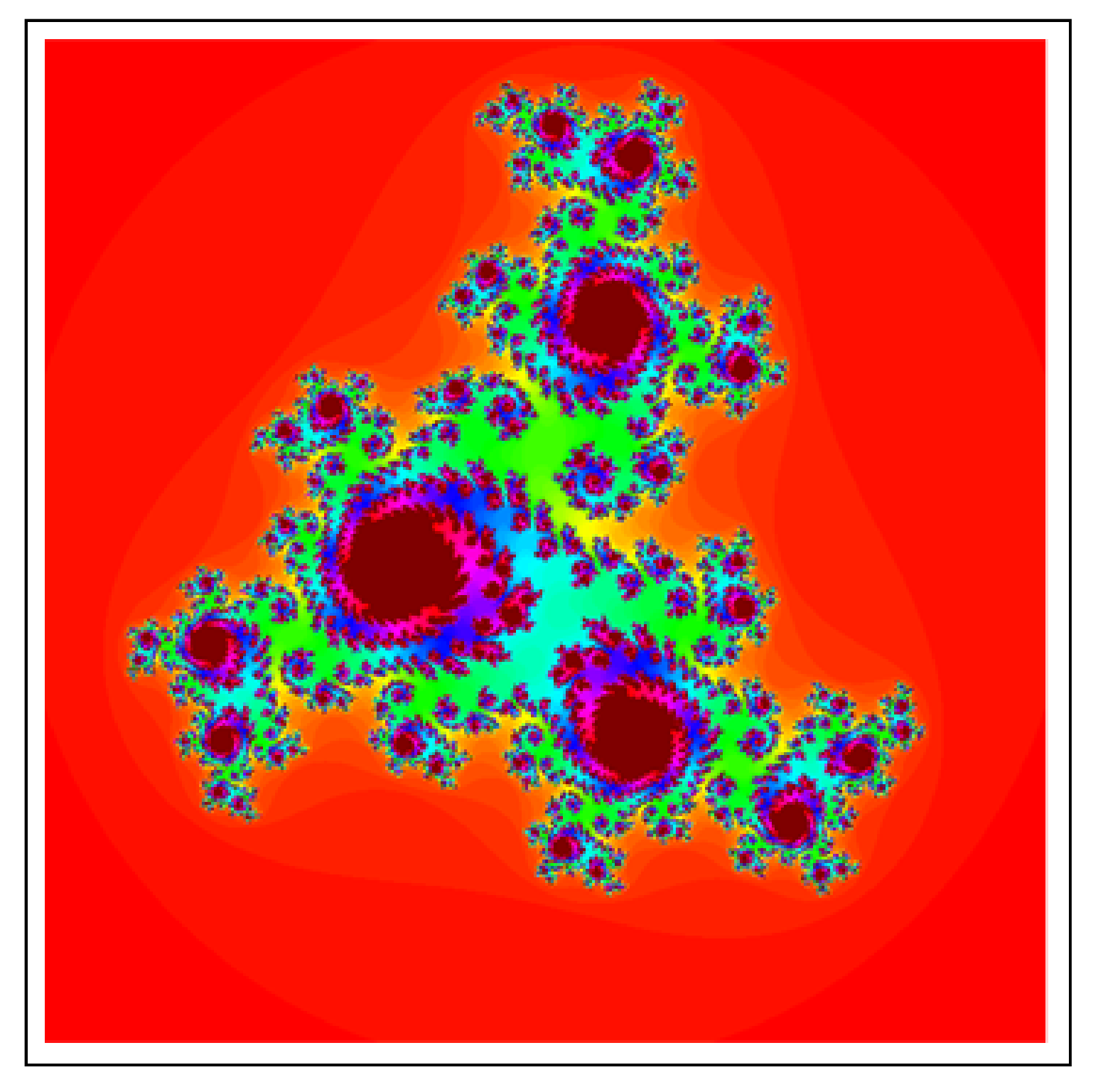
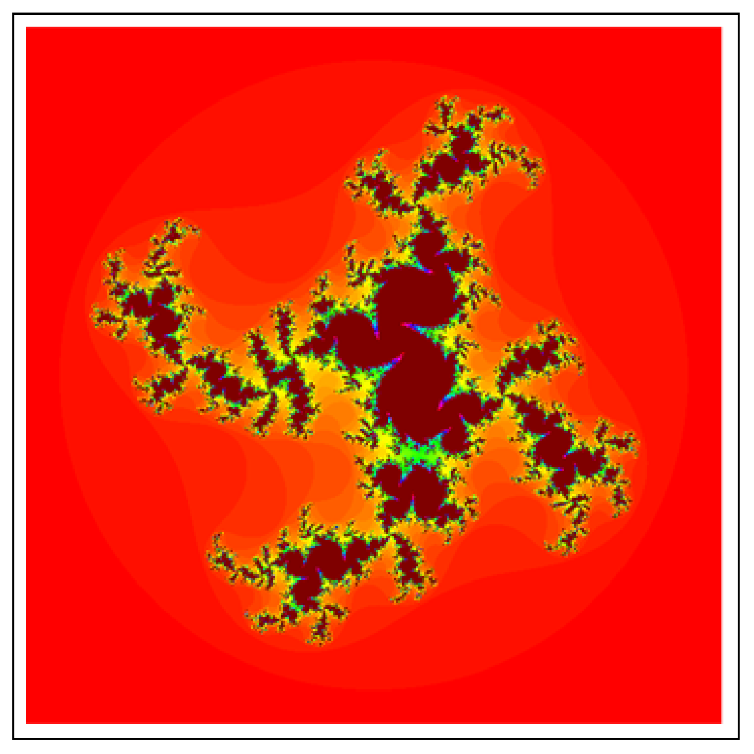
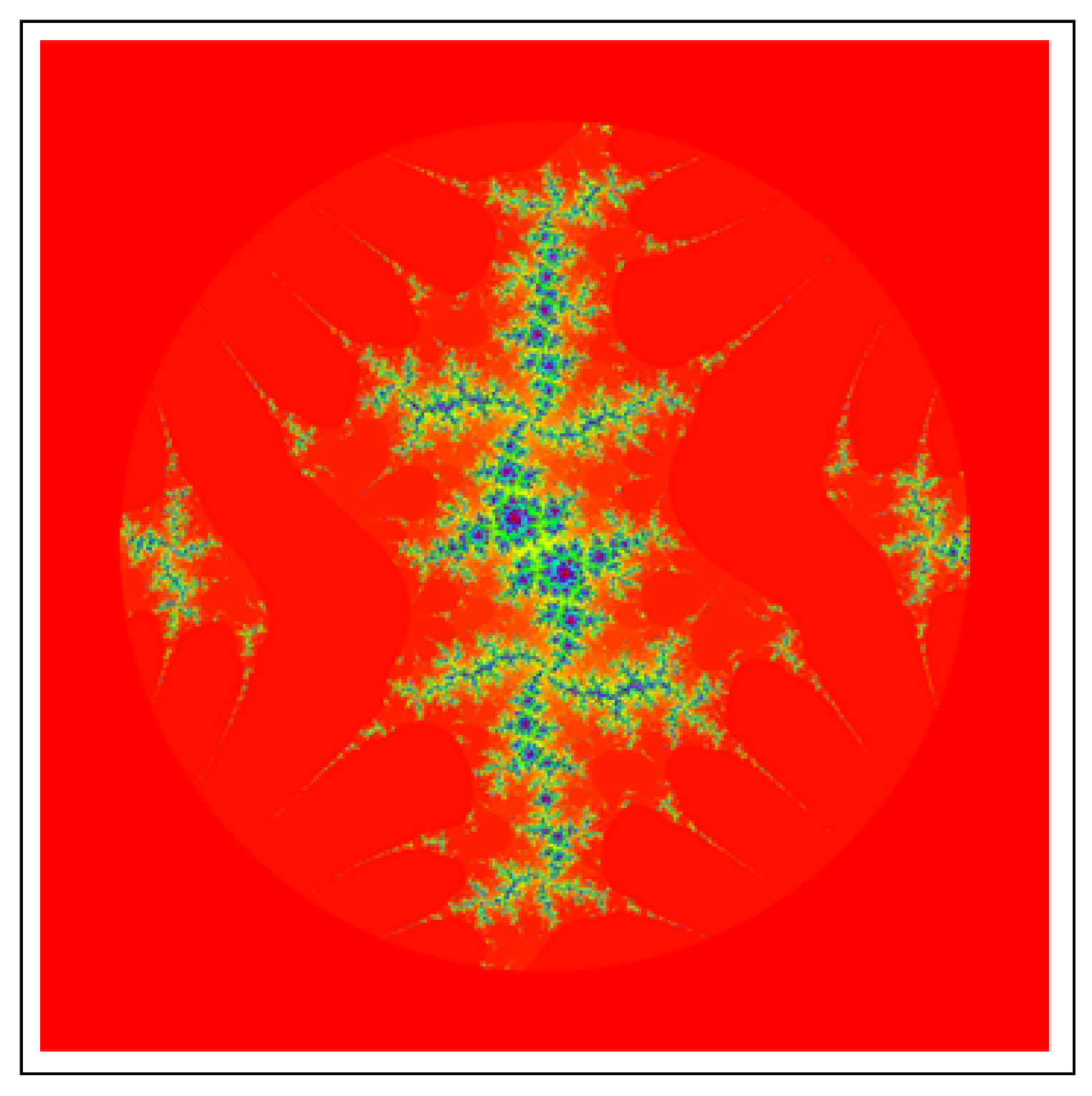
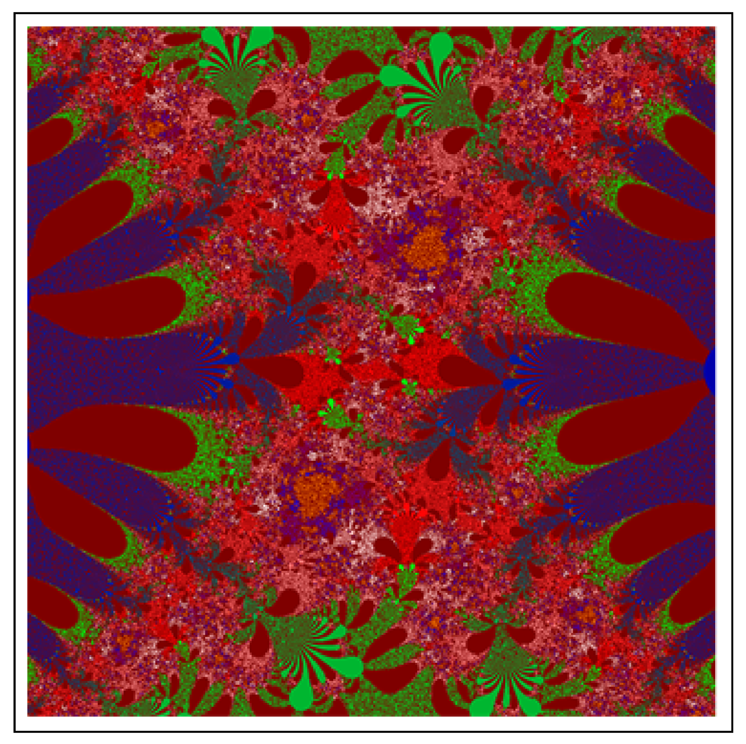
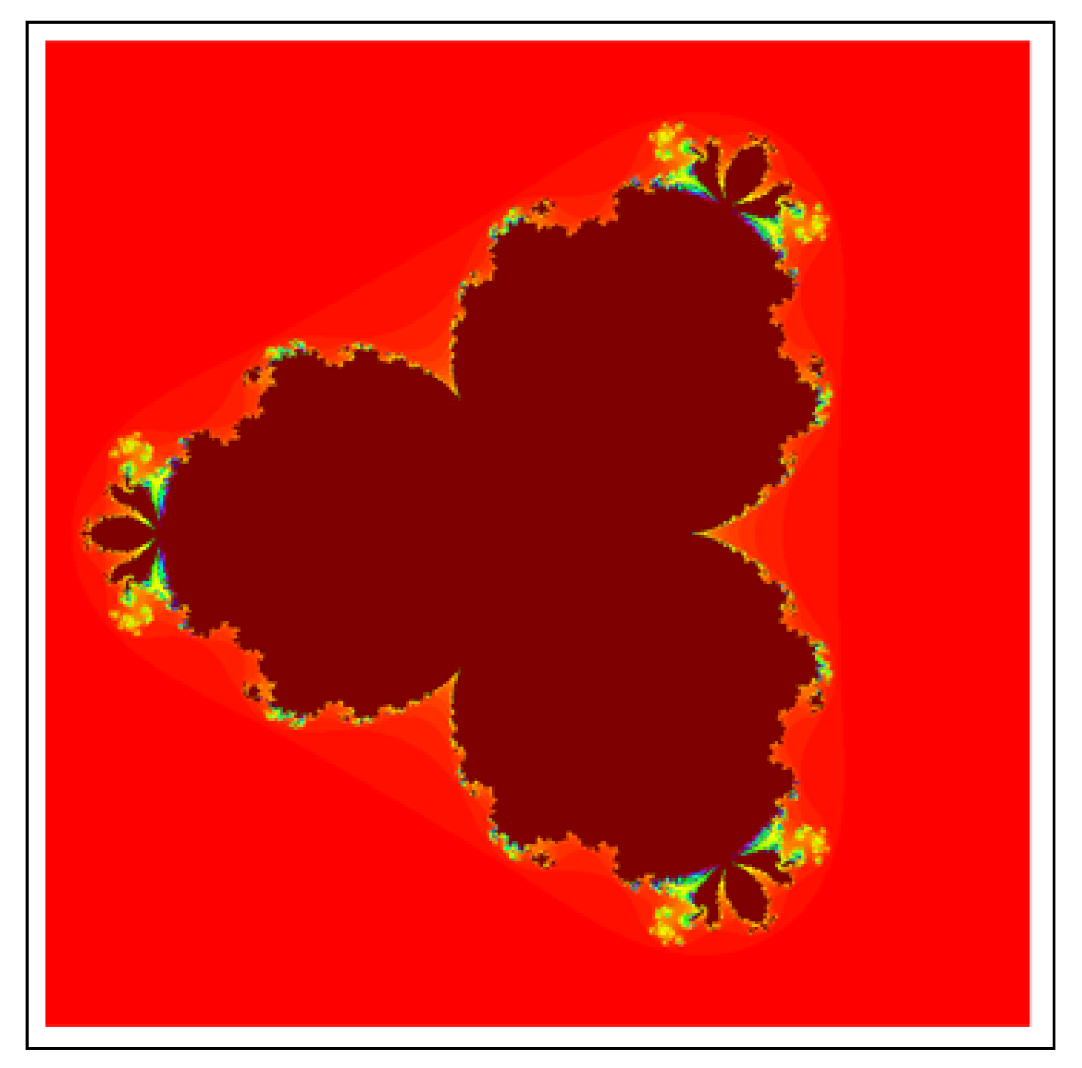
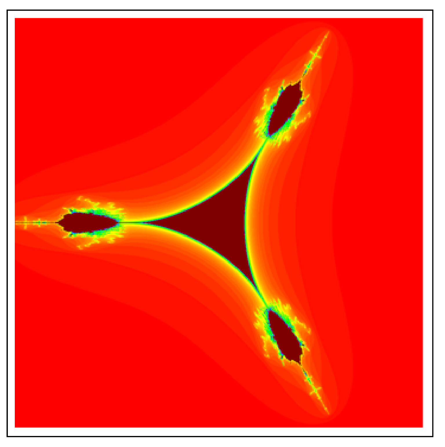
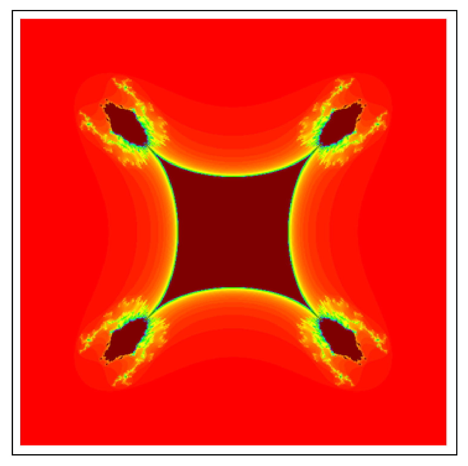
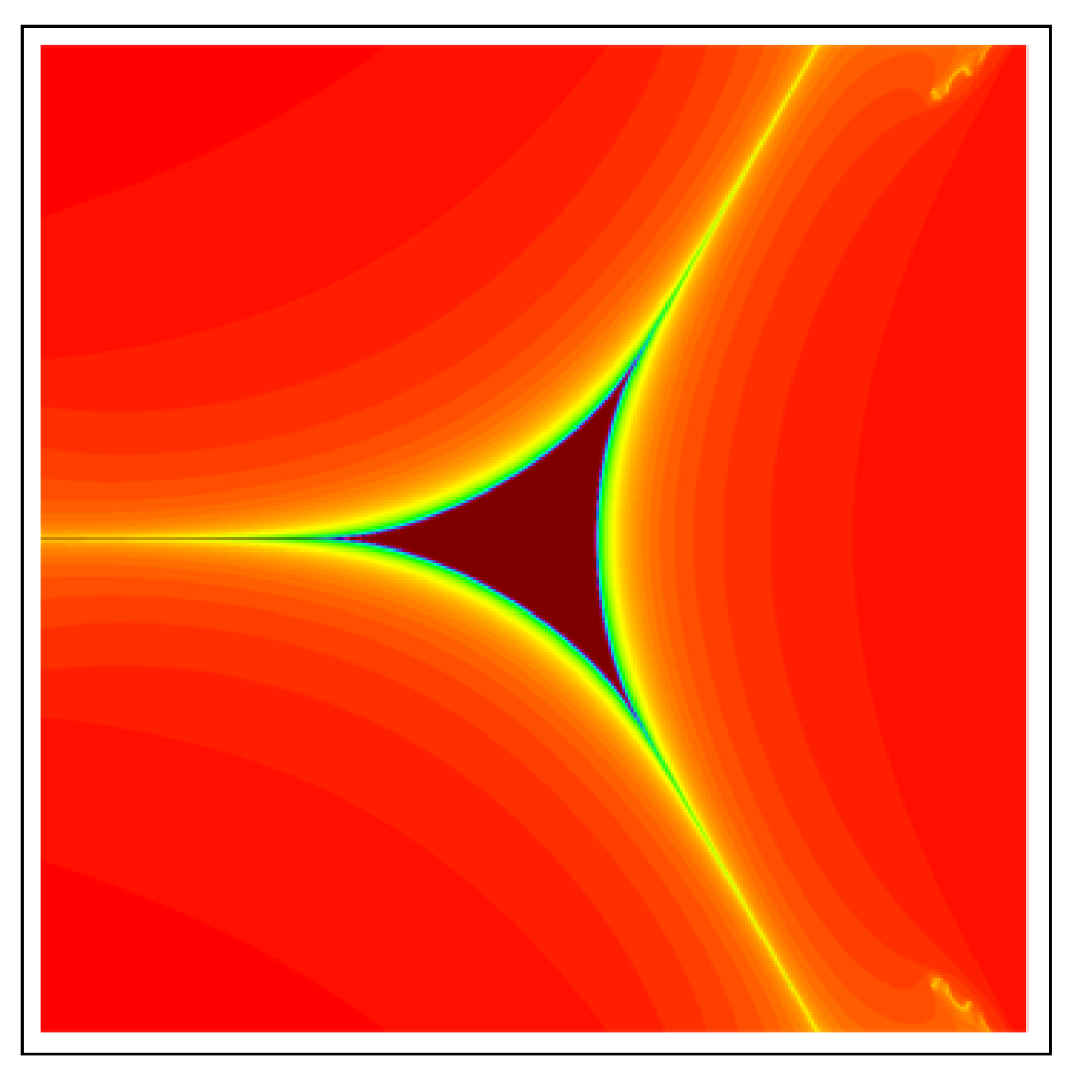
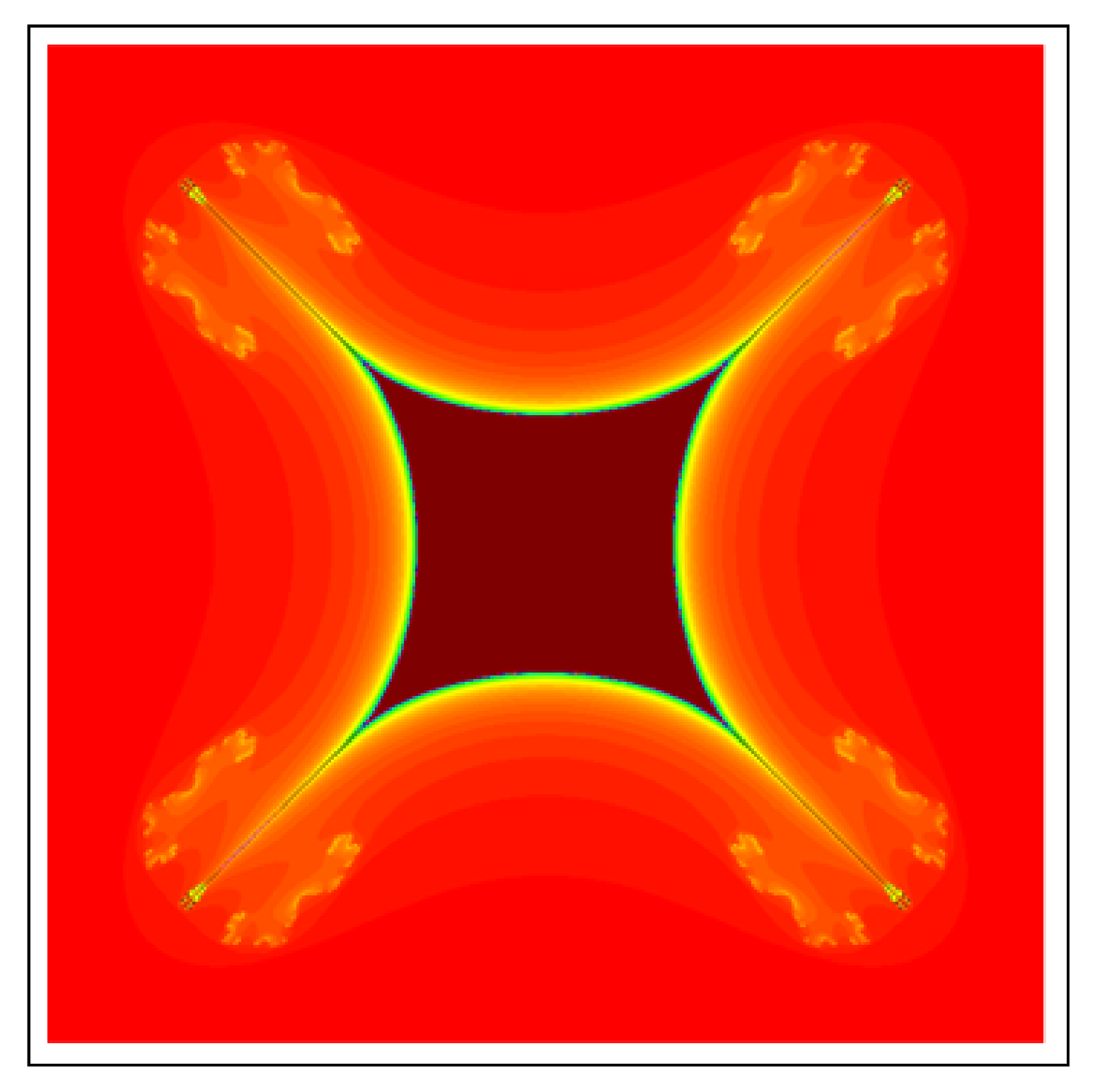
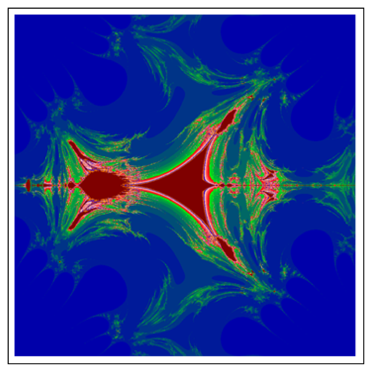
4.1. Julia Set

In this part, we explain some J-sets for the polynomials $h\left(z\right)=z^n+c$, $h\left(z\right)=sin\left(z^n\right)+c$ and $h\left(z\right)=e^{z^n}+c$ at different n in the orbit of F-iteration. We generated Julia sets for $n=2$, $n=3$ and $n=3$ via F-iterative scheme. For each graph, we set $I=100$ (i.e., the highest number of iterates) in Algorithm 1.

Example 1. 

In this example, we present Julia sets for the function $h\left(z\right)=z^n+c$ at n = 2, 3 and 4. In Figure 1, Figure 2 and Figure 3, we fix $\alpha =0.9$ and change the values of c. In Figure 4, Figure 5 and Figure 6, we fix the parameter $\alpha =0.8$ and change the values of c. In Figure 7, Figure 8 and Figure 9, we fix the value of $\alpha =0.7$ for different values of c. In Figure 10, we fix the value of $\alpha =0.6$ for different values of $c=0.56+0.9I$. We set the occupied area $A={[-1.5,1.5]}^2$. We noted the generation time of all images in seconds and noticed that while increasing the value of n and decreasing the occupied area, images take less time for generation. Quadratic Julia sets take more generation time than Cubic and Bi-quadratic.

Algorithm 1: Geometry of Julia Set

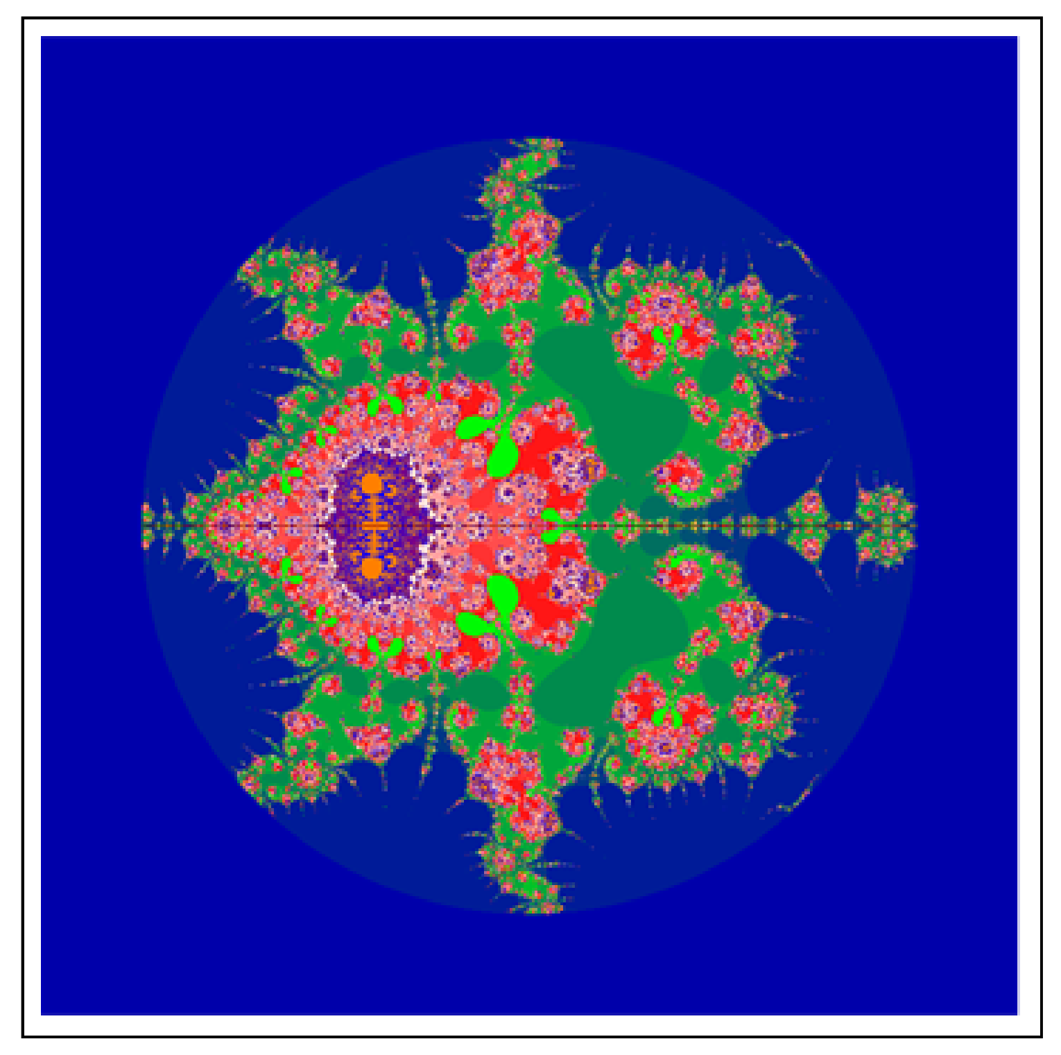
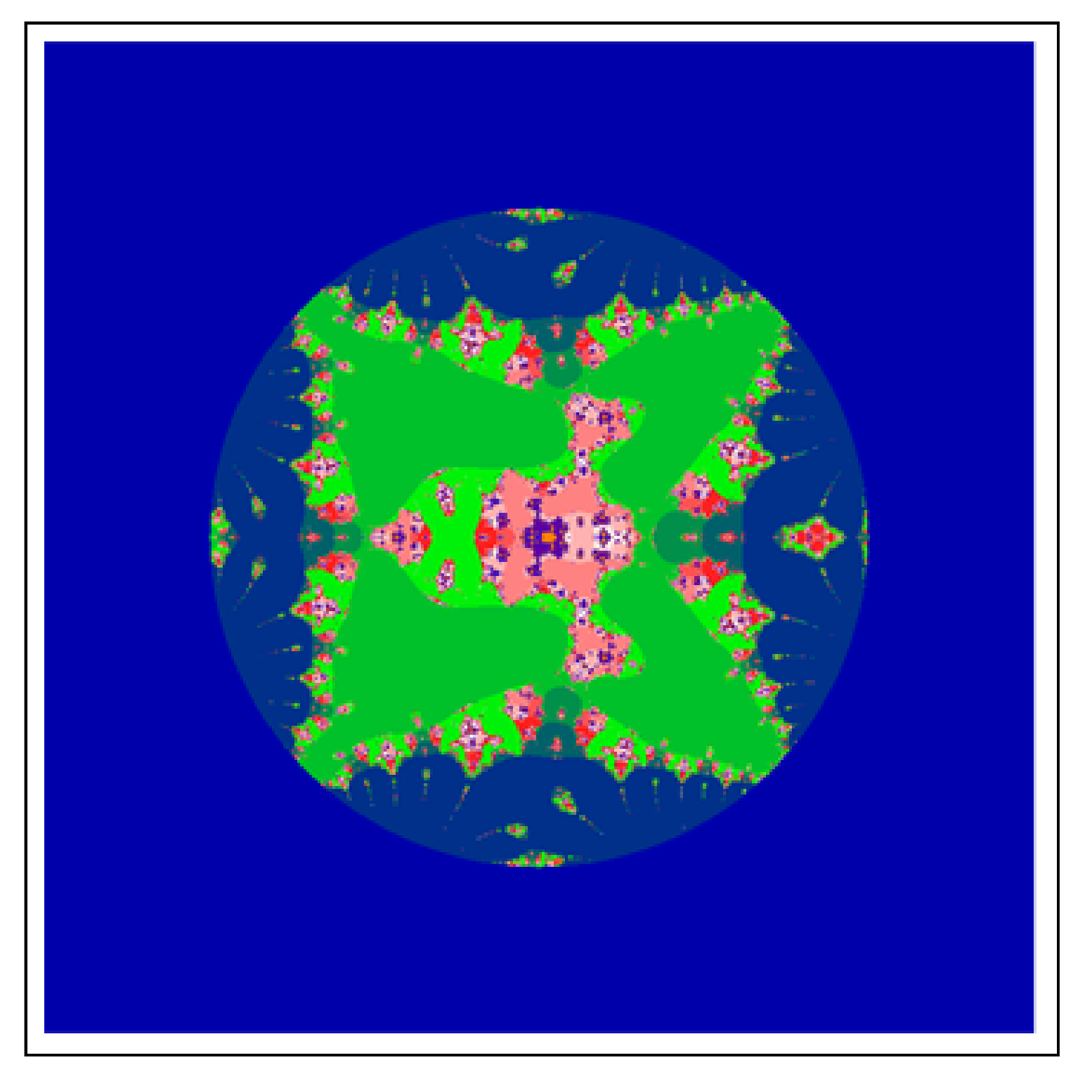
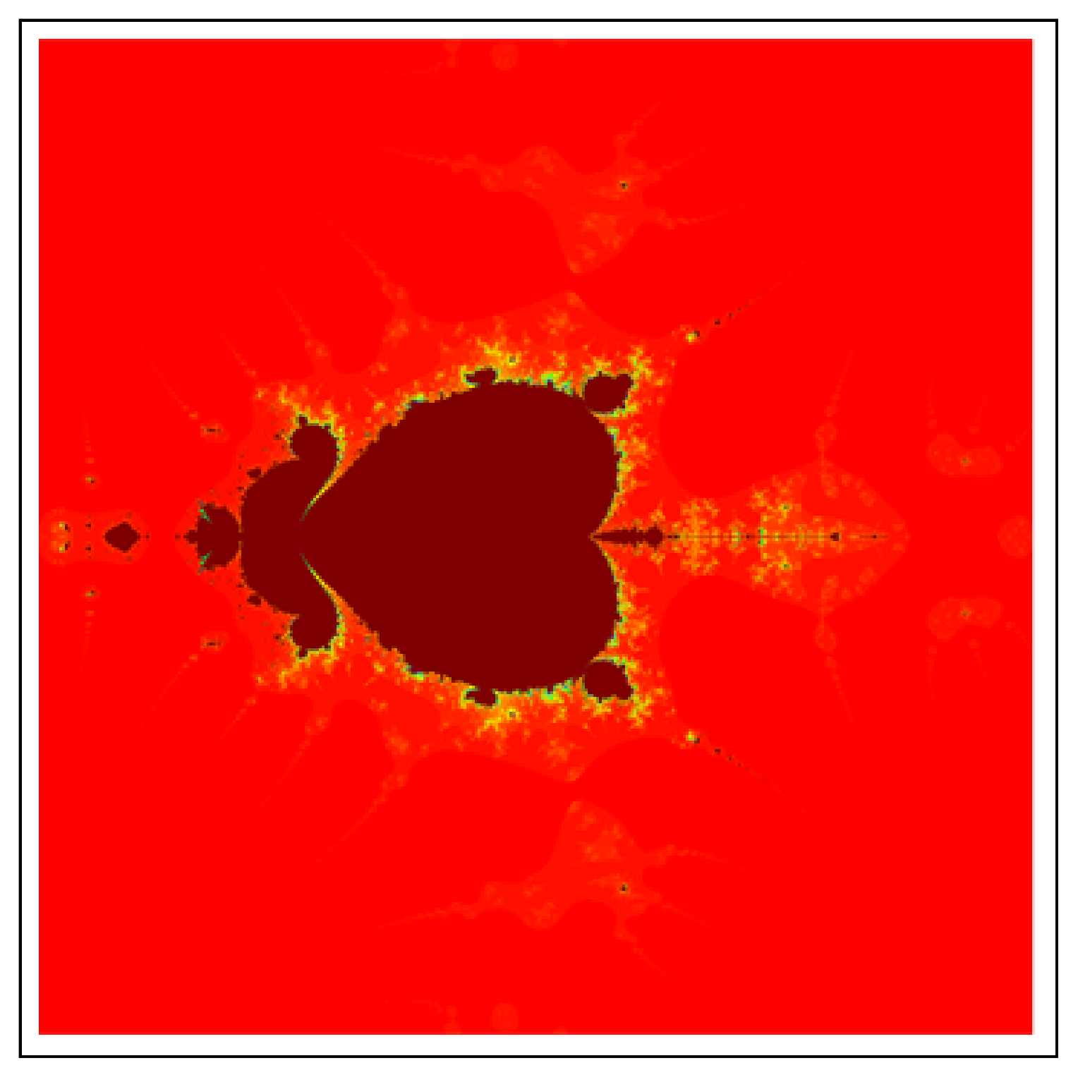
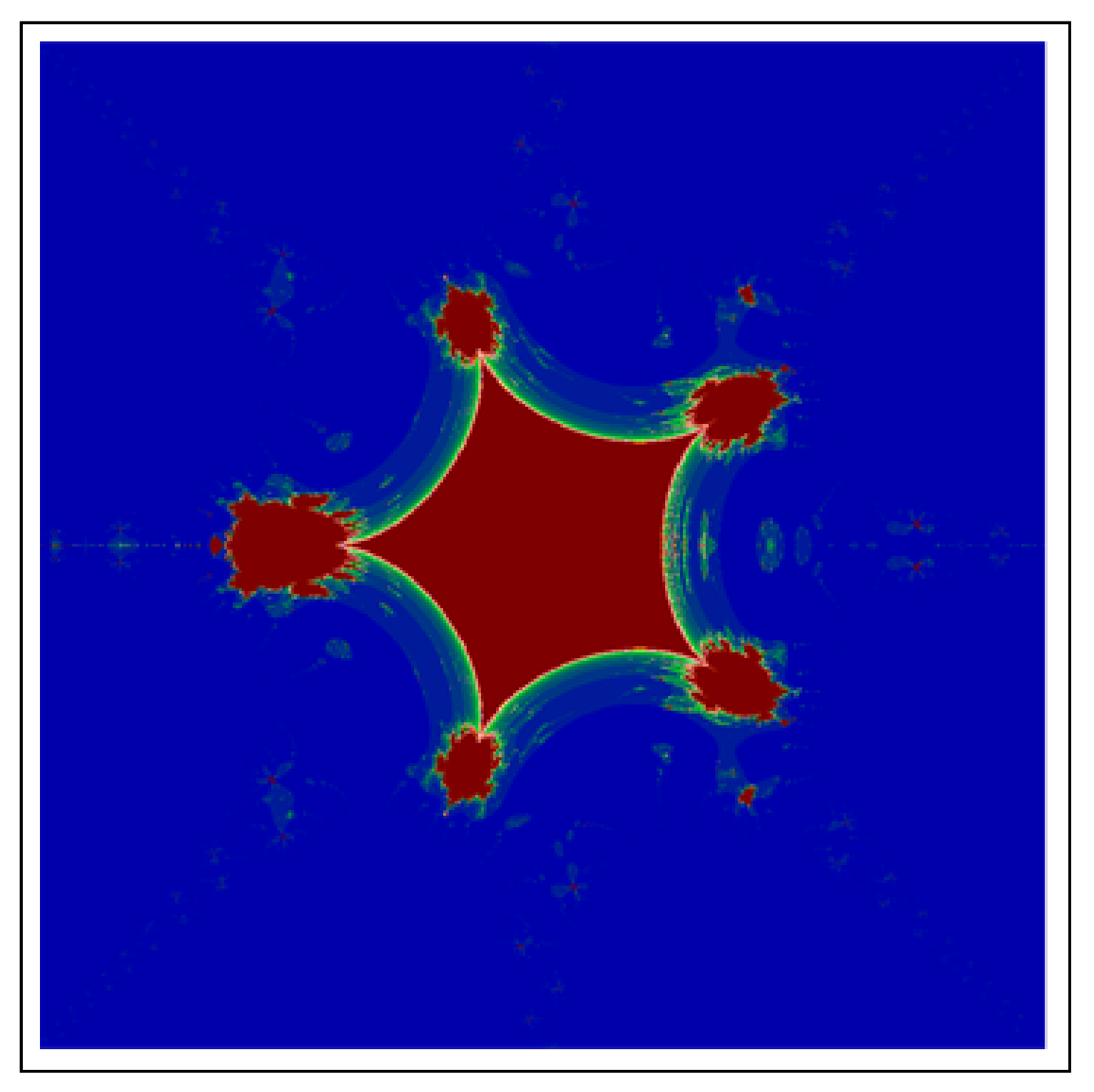
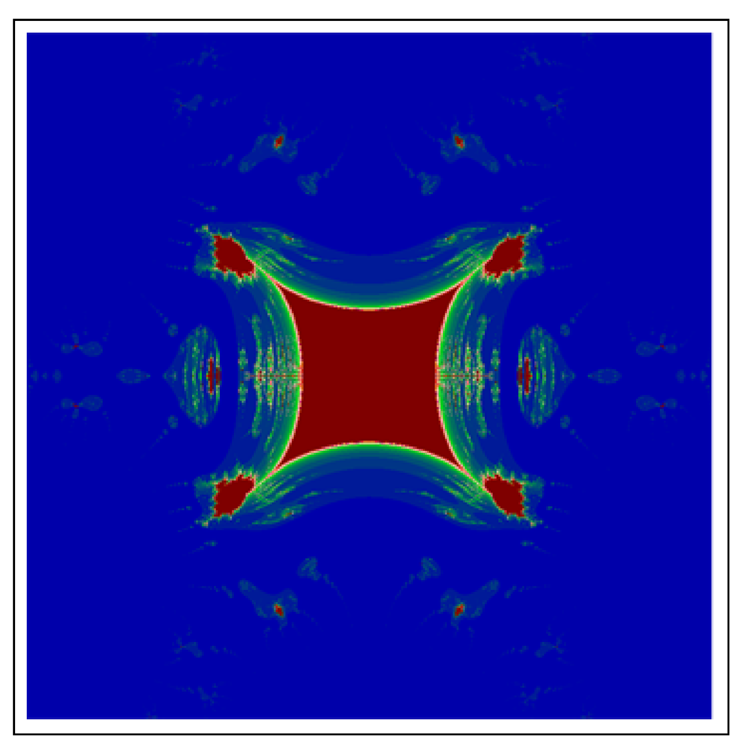
Algorithm 2: Geometry of M-Set

Example 2. 

In this example, we present Julia sets for the function $h\left(z\right)=sin\left(z^n\right)+c$ at n = 2, 3 and 4. In Figure 11 and Figure 12, we fix $\alpha ,|{\eta }_1|,|{\eta }_2|,|{\eta }_3|,|{\eta }_4|=0.8$ and the values of $c=1.09$. In Figure 13 and Figure 14, we fix $\alpha ,|{\eta }_1|,|{\eta }_2|,|{\eta }_3|,|{\eta }_4|=0.95$ and the values of $c=0.3-0.7i$ and $c=0.55$, respectively. In Figure 15, Figure 16 and Figure 17, we fix $\alpha ,|{\eta }_1|,|{\eta }_2|,|{\eta }_3|,|{\eta }_4|=0.5$ and the values of $c=0.5+0.75i$, $c=0.51$ and $c=0.55$, respectively. In Figure 18 and Figure 19, we fix $\alpha ,|{\eta }_1|,|{\eta }_2|,|{\eta }_3|,|{\eta }_4|=0.85$ and the values of $c=0.51$ and $c=0.55$, respectively. For $n=2$ set, we set area $A={[-2,5,2.5]}^2$, and for $n=3,4$ J-sets, area $A={[-2,2]}^2$. In Figure 20, Figure 21, Figure 22, Figure 23, Figure 24 and Figure 25, we present J-sets for the function $h\left(z\right)=e^{z^n}+c$ at n = 2, 3 and 4. In Figure 20, Figure 21 and Figure 22, we fix $\alpha ,|{\eta }_1|,|{\eta }_2|,|{\eta }_3|,|{\eta }_4|=0.009$, and in Figure 23, Figure 24 and Figure 25, we fix $\alpha ,|{\eta }_1|,|{\eta }_2|,|{\eta }_3|,|{\eta }_4|=0.001$. We set occupied area $A={[-2.5,2.5]}^2$ and noted the generation time of all images in seconds.

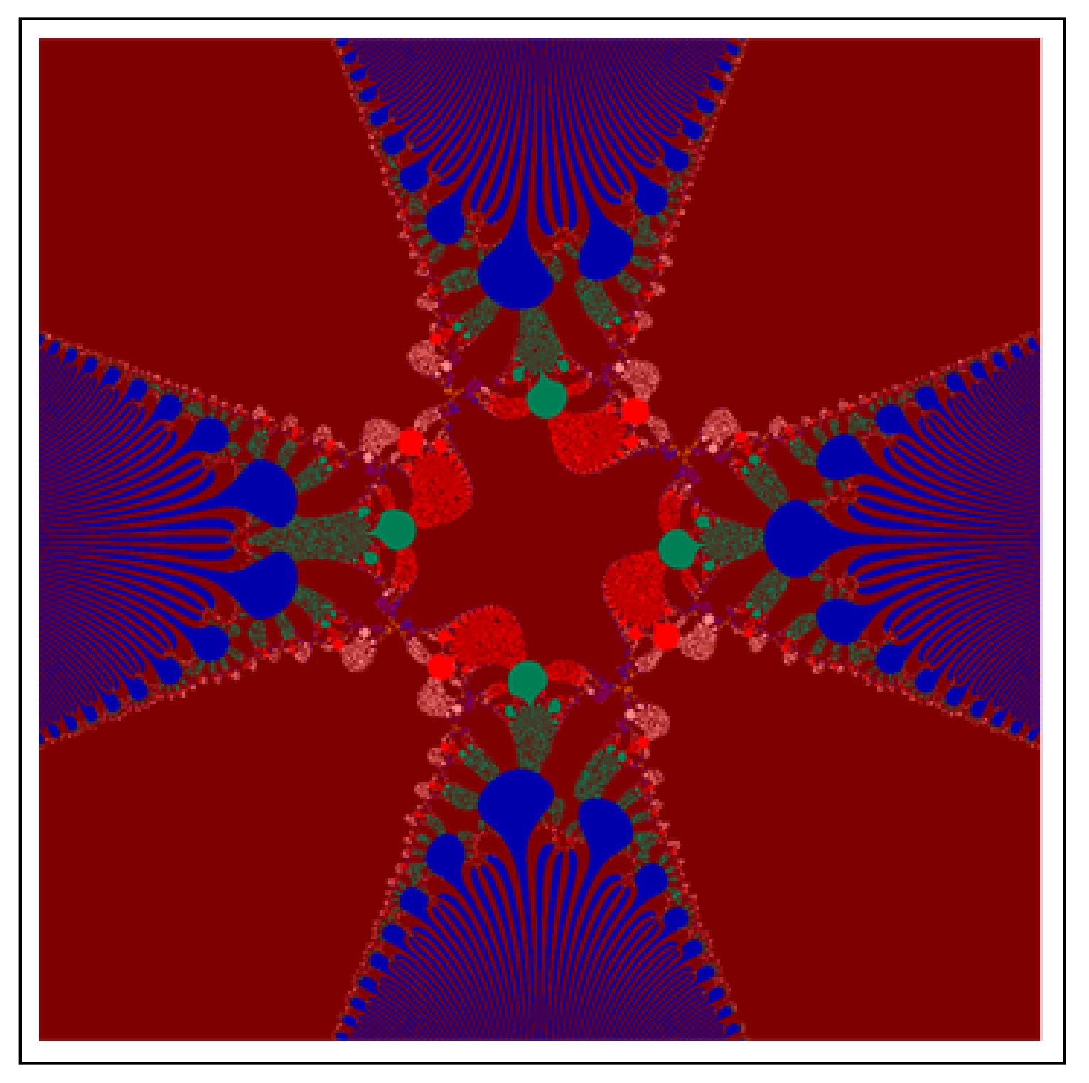
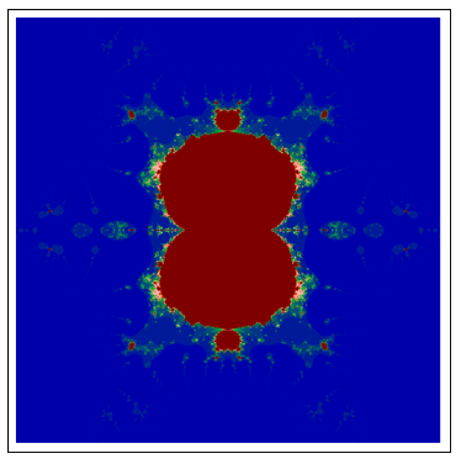
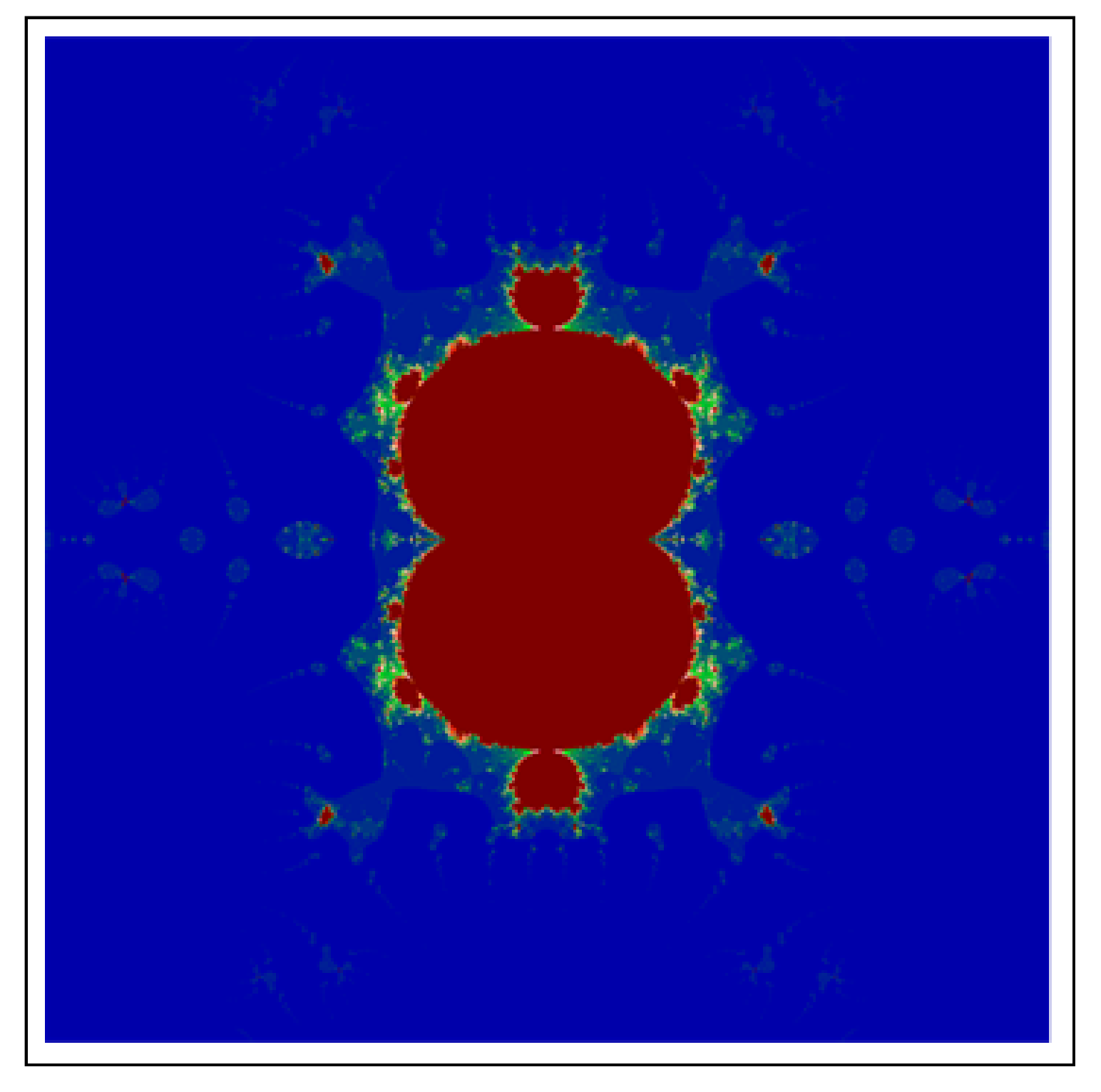
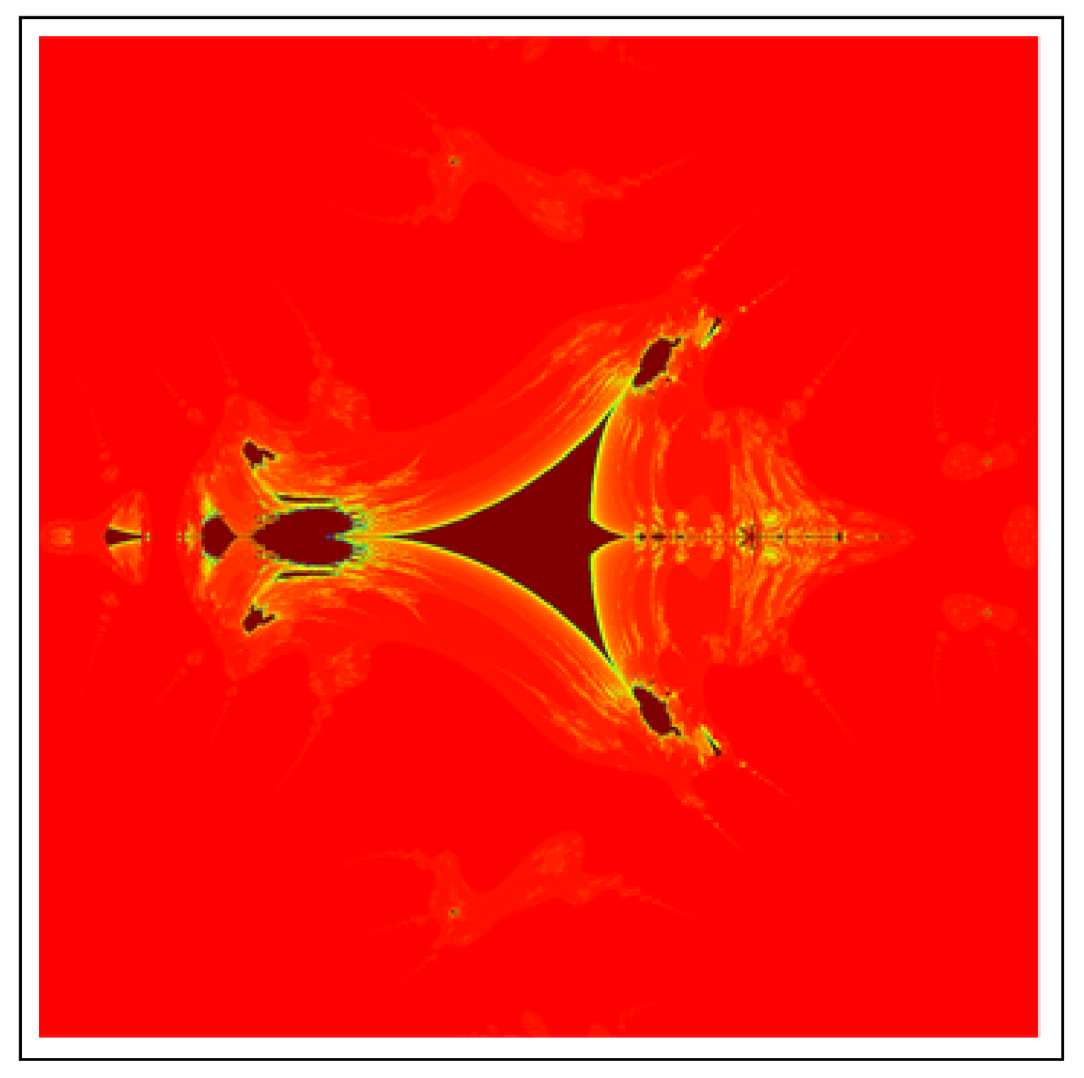
Algorithm 3: Geometry of Multi-corn

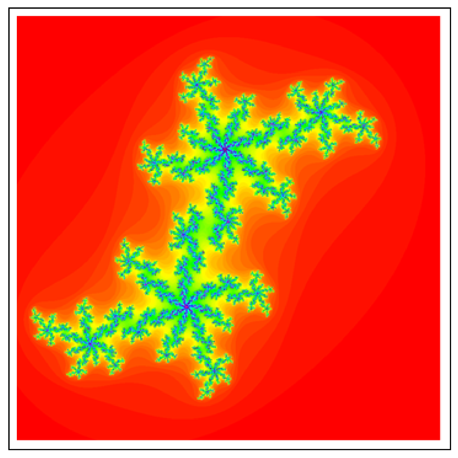
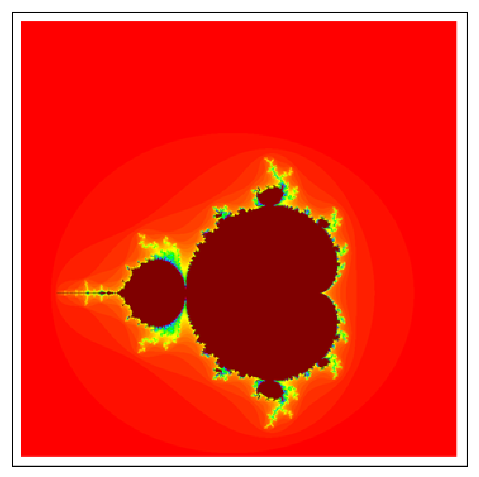
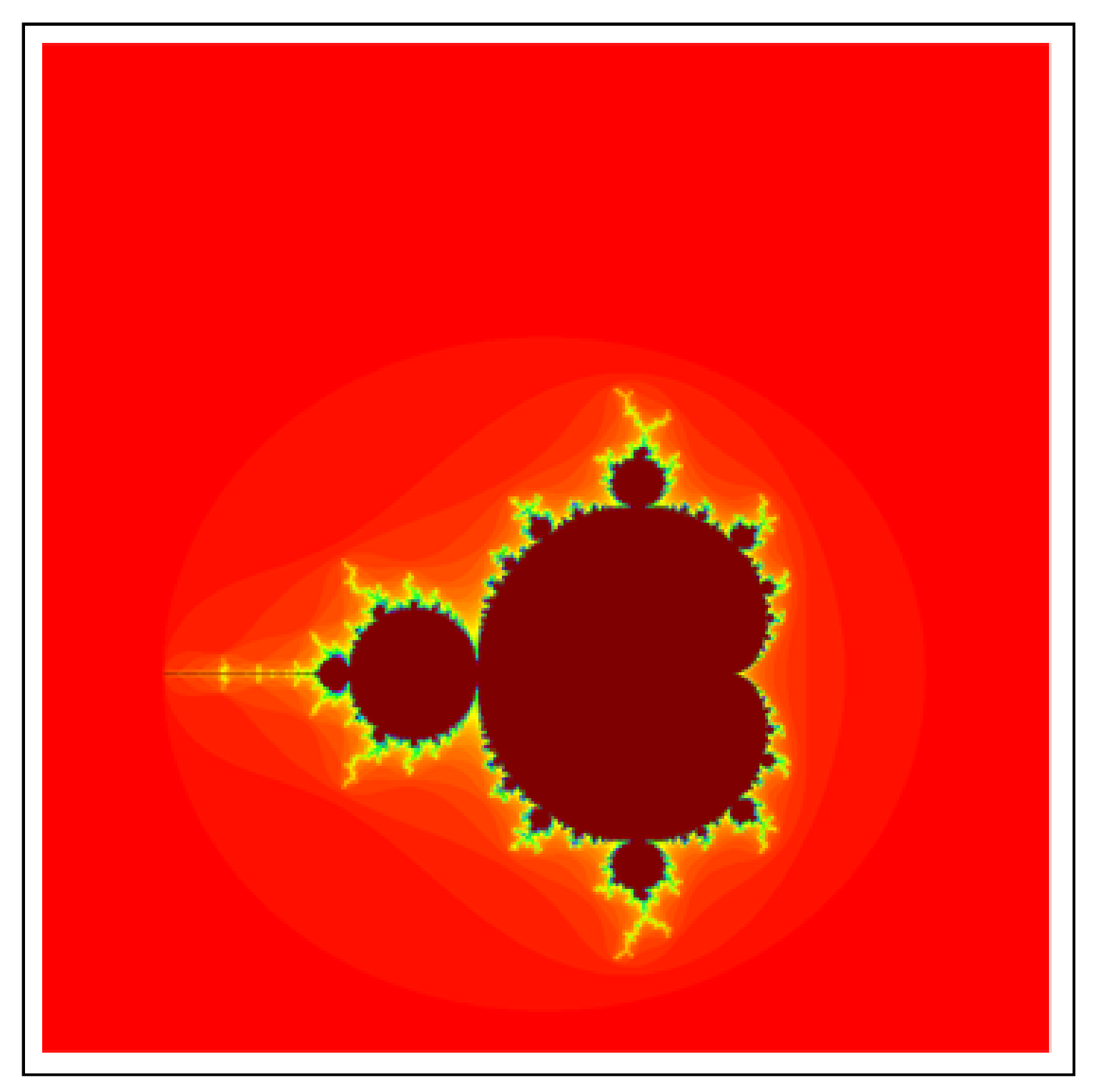
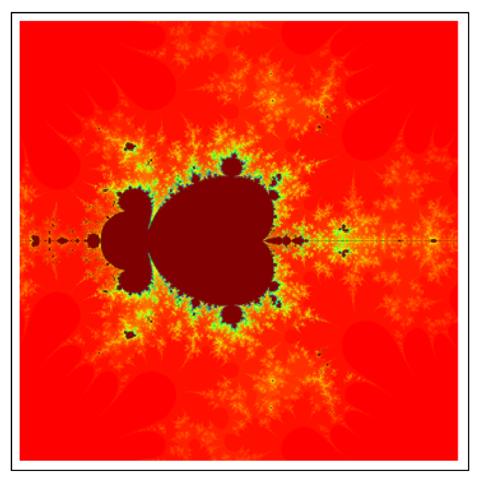
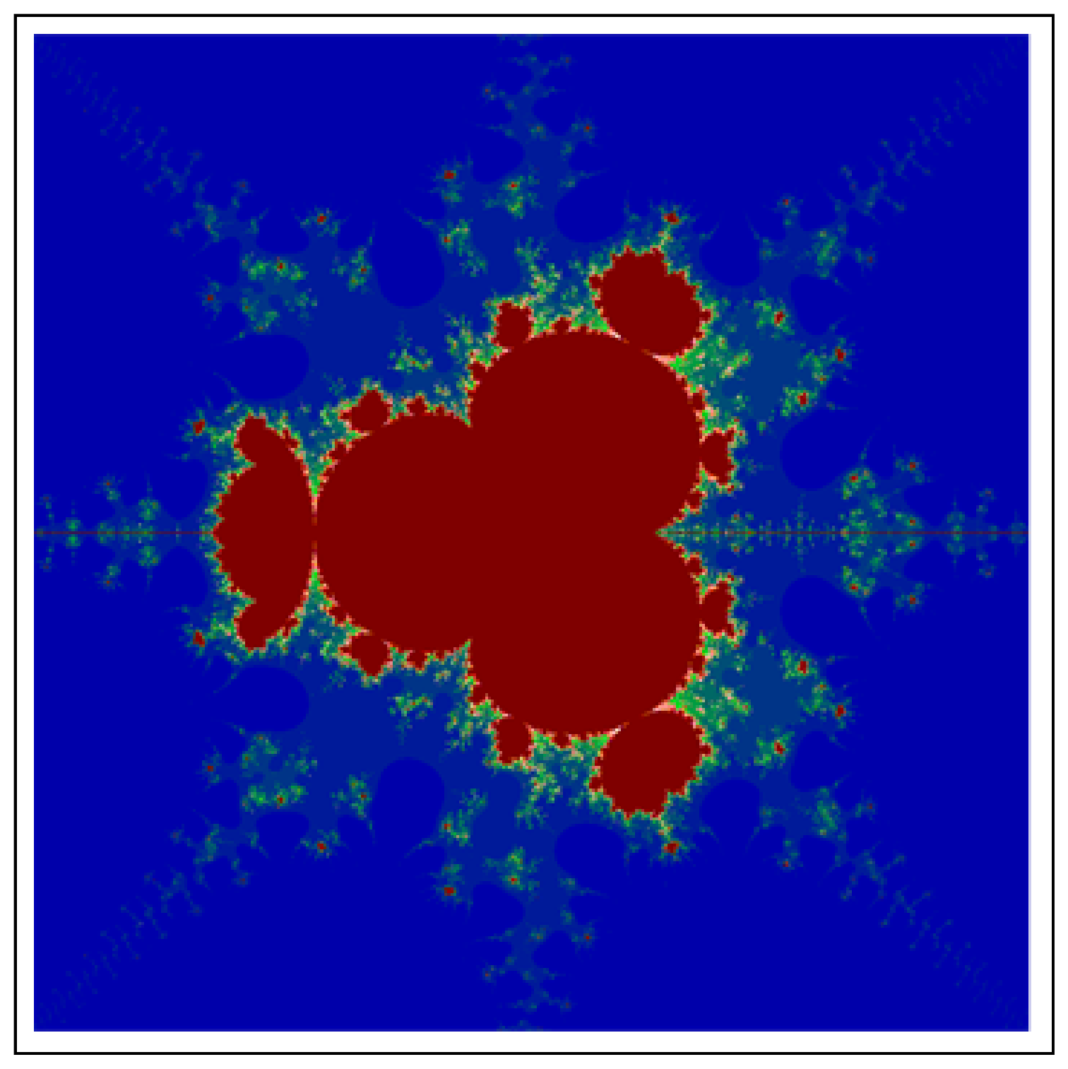
4.2. Mandelbrot Set

Here, we discuss some Mandelbrot sets for the functions $h\left(z\right)=z^n+c$, $h\left(z\right)=sin\left(z^n\right)+c$ and $h\left(z\right)=e^{z^n}+c$ at different n in the orbit of proposed iteration. We have generated Mandelbrot sets for $n=2,3,4$ via F-iteration. In all graphs, we set $I=100$ (i.e., the highest number of iterates) in Algorithm 2.

Example 3. 

Here, we explain M-sets for the function $h\left(z\right)=z^n+c$ at n = 2, 3 and 4. In Figure 26, Figure 27 and Figure 28, we fix the parameter $\alpha =0.9$. In Figure 29, Figure 30 and Figure 31, we fix the parameter $\alpha =0.8$. In Figure 32 and Figure 33, we fix the parameter $\alpha =0.99$. In Figure 34, we fix the parameters $\alpha =0.7$. In Figure 35, we fix the parameters $\alpha =0.1$. We set the occupied area $A={[-1.5,1.5]}^2$. We noted the generation time of all images in seconds and noticed that while increasing the value n and decreasing the occupied area, images take less time for generation. Quadratic Mandelbrot sets take more generation time than Cubic and Bi-quadratic.

Example 4. 

In this example, we explain M-sets for the function $h\left(z\right)=sin\left(z^n\right)+c$ at n = 2, 3 and 4. In Figure 36, we fix the parameters $\alpha ,|{\eta }_1|,|{\eta }_2|,|{\eta }_3|,|{\eta }_4|=0.8$. In Figure 37 and Figure 38, we fix the parameters $\alpha ,|{\eta }_1|,|{\eta }_2|,|{\eta }_3|,|{\eta }_4|=0.7$. In Figure 39 and Figure 40, we fix the parameters $\alpha ,|{\eta }_1|,|{\eta }_2|,|{\eta }_3|,|{\eta }_4|=0.85$. In Figure 41, Figure 42 and Figure 43, we fix the parameters $\alpha ,|{\eta }_1|,|{\eta }_2|,|{\eta }_3|,|{\eta }_4|=0.07$. In Figure 44, we fix the parameters $\alpha ,|{\eta }_1|,|{\eta }_2|,|{\eta }_3|,|{\eta }_4|=0.95$. In Figure 45, we fix the parameters $\alpha ,|{\eta }_1|,|{\eta }_2|,|{\eta }_3|,|{\eta }_4|=0.009$. In Figure 46, we fix the parameters $\alpha ,|{\eta }_1|,|{\eta }_2|,|{\eta }_3|,|{\eta }_4|=0.001$. We set the occupied area $A={[-2.5,2.5]}^2$. We noted the generation time of all images in seconds and noticed that while increasing the value n and decreasing the occupied area, images take less time for generation.

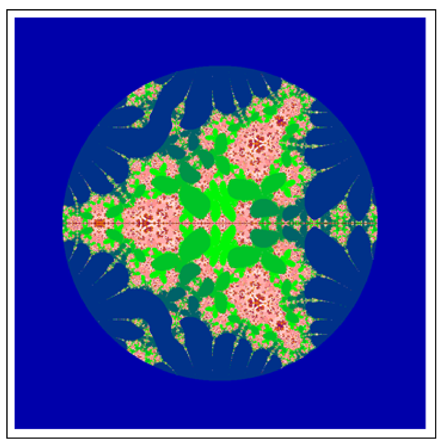
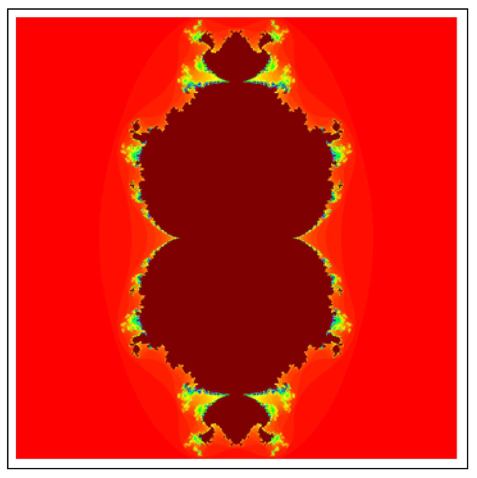
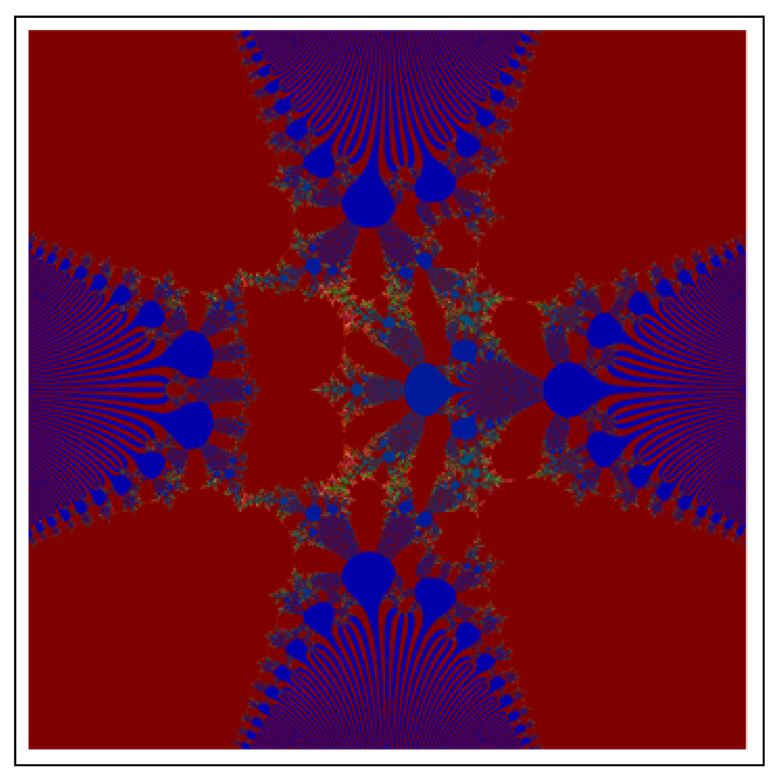
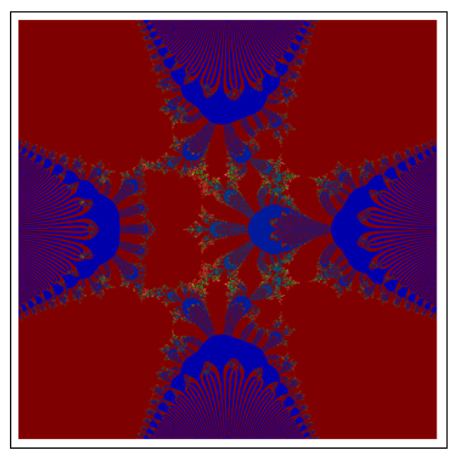
4.3. Multi-Corn

Here, we discuss some multibrot set for for the polynomial $h\left(z\right)={\overline{z}}^n+c$ at n = 2, 3 and 4. We noticed that for $n=2$, Multi-corns become tricorns. We noted the generation time of each figure. We fixed the number of iteration up to 100 for each image in Algorithm 3.

Example 5. 

Here, we explain Multi-corns for the function $h\left(z\right)={\overline{z}}^n+c$ at n = 2, 3 and 4. In Figure 47, Figure 48 and Figure 49, we fix the parameter $\alpha =0.9$. In Figure 50, Figure 51 and Figure 52, we fix the parameter $\alpha =0.8$. In Figure 53, Figure 54 and Figure 55, we fix the parameter $\alpha =0.7$. We noticed that the tricorn is three-cornered and the style of its self similarity is exactly the same as that of the Mandelbrot set. All Multi-corns have $n+1$ lashes.

Example 6. 

In this example, we present Multi-corns for the function $h\left(z\right)=sin{\overline{z}}^n+c$ at n = 2, 3 and 4. In Figure 56, Figure 57 and Figure 58, we fix the parameters $\alpha ,|{\eta }_1|,|{\eta }_2|,|{\eta }_3|,|{\eta }_4|=0.85$. In Figure 59 and Figure 60, we fix the parameters $\alpha ,|{\eta }_1|,|{\eta }_2|,|{\eta }_3|,|{\eta }_4|=0.0.07$. In Figure 61, we fix the parameters $\alpha ,|{\eta }_1|,|{\eta }_2|,|{\eta }_3|,|{\eta }_4|=0.0.7$. In Figure 62, we fix the parameters $\alpha ,|{\eta }_1|,|{\eta }_2|,|{\eta }_3|,|{\eta }_4|=0.95$. For Tricorns, we set area $A={[-2.5.2.5]}^2$; for Multi-corns, we set area $A={[-2,2]}^2$.

5. Conclusions

We proved escape criterion for a complex function $h\left(z\right)=z^n+c$, complex trigonometric function $h\left(z\right)=sin\left(z^n\right)+c$ and complex exponential function $h\left(z\right)=e^{z^n}+c$ with $n\ge 2$ and $c\in \mathbb{C}$ via F-iteration. We used the established results in Algorithms 1–3 for the Julia sets, Mandelbrot sets and Multi-corns in the orbit of our proposed iteration. We generated Quadratic, Cubic and Bi-quadratic Julia Mandelbrot sets, and some Tricorns and Multi-corns.

References

- Barnsley, M. Fractals Everywhere; Morgan Kaufmann Publishers: Burlington, MA, USA, 1993. [Google Scholar]
- Mandelbrot, B.B. The Fractal Geometry Nature; Freeman: New York, NY, USA, 1982; Volume 2. [Google Scholar]
- Lakhtakia, A.; Varadan, W.; Messier, R.; Varadan, V.K. On the symmetries of the Julia sets for the process zp + c. J. Phys. A Math. Gen. 1987, 20, 3533–3535. [Google Scholar] [CrossRef]
- Crowe, W.D.; Hasson, R.; Rippon, P.J.; Strain-Clark, P.E.D. On the structure of the Mandelbar set. Nonlinearity 1989, 2, 541. [Google Scholar] [CrossRef]
- Kim, T. Quaternion Julia set shape optimization. Comput. Graph. Forum 2015, 34, 167–176. [Google Scholar] [CrossRef]
- Drakopoulos, V.; Mimikou, N.; Theoharis, T. An overview of parallel visualisation methods for mandelbrot and Julia sets. Comput. Graph. 2003, 27, 635–646. [Google Scholar] [CrossRef]
- Rani, M.; Agarwal, R. Effect of stochastic noise on superior Julia sets. J. Math. Imag. Vis. 2010, 36, 63. [Google Scholar] [CrossRef]
- Prasad, B.; Katiyar, K. Fractals via Ishikawa iteration. In Proceedings of the International Conference on Logic, Information, Control and Computation, Gandhigram, India, 25–27 February 2011; pp. 197–203. [Google Scholar]
- Kang, S.M.; Rafiq, A.; Latif, A.; Shahid, A.A.; Kwun, Y.C. Tricorns and Multi-corns of S-iteration scheme. J. Funct. Spaces 2015, 2015, 1–7. [Google Scholar]
- Ashish, M.R.; Chugh, R. Julia sets and mandelbrot sets in Noor orbit. Appl. Math. Comput. 2014, 228, 615–631. [Google Scholar] [CrossRef]
- Phuengrattana, W.; Suantai, S. On the rate of convergence of Mann, Ishikawa, Noor and SP-iterations for continuous functions on an arbitrary interval. J. Comput. Appl. Math. 2011, 235, 3006–3014. [Google Scholar] [CrossRef]
- Chugh, R.; Kumar, V.; Kumar, S. Strong convergence of a new three step iterative scheme in Banach spaces. Amer. J. Comput. Math. 2012, 2, 345. [Google Scholar] [CrossRef]
- Kwun, Y.C.; Tanveer, M.; Nazeer, W.; Abbas, M.; Kang, S.M. Fractal generation in modified Jungck–S orbit. IEEE Access 2019, 7, 35060–35071. [Google Scholar] [CrossRef]
- Kwun, Y.C.; Tanveer, M.; Nazeer, W.; Gdawiec, K.; Kang, S.M. Mandelbrot and Julia sets via Jungck-CR iteration with s-convexity. IEEE Access 2019, 7, 12167–12176. [Google Scholar] [CrossRef]
- Li, D.; Tanveer, M.; Nazeer, W.; Guo, X. Boundaries of filled Julia sets in generalized Jungck-Mann orbit. IEEE Access 2019, 7, 76859–76867. [Google Scholar] [CrossRef]
- Li, X.; Tanveer, M.; Abbas, M.; Ahmad, M.; Kwun, Y.C.; Liu, J. Fixed point results for fractal generation in extended Jungck-SP orbit. IEEE Access 2019, 7, 160472–160481. [Google Scholar] [CrossRef]
- Pickover, C.A. Biom orphs: Computer displays of biological forms generated from mathematical feedback loops. Comput. Graph. Forum 1986, 5, 313–316. [Google Scholar] [CrossRef]
- Gdawiec, K.; Kotarski, W.; Lisowska, A. Biomorphs via modified iterations. J. Nonlinear Sci. Appl. 2016, 9, 2305–2315. [Google Scholar] [CrossRef]
- Alonso-Sanz, R. Biomorphs with memory. Int. J. Parallel Emergent Distrib. Syst. 2018, 33, 1–11. [Google Scholar] [CrossRef]
- Qi, H.; Tanveer, M.; Nazeer, W.; Chu, Y. Fixed Point Results for Fractal Generation of Complex Polynomials Involving Sine Function via Non-Standard Iterations. IEEE Access 2020, 8, 154301–154317. [Google Scholar] [CrossRef]
- Wang, W.; Hu, X.; Shahid, A.A.; Wang, M. Generation of Antifractals via Hybrid Picard-Mann Iteration. IEEE Access 2020, 8, 83974–83985. [Google Scholar] [CrossRef]
- Ali, J.; Ali, F. A new iterative scheme for approximating fixed points with an application to a delay diferential equation. J. Nonlinear Convex Anal. 2020, 21, 2151–2163. [Google Scholar]
- Devaney, R. A First Course in Chaotic Dynamical Systems: Theory and Experiment; Addison-Wesley: New York, NY, USA, 1992. [Google Scholar]
- Liu, X.; Zhu, Z.; Wang, G.; Zhu, W. Composed accelerated escape time algorithm to construct the general mandelbrot sets. Fractals 2001, 9, 149–153. [Google Scholar] [CrossRef]
- Mann, W.R. Mean value methods in iteration. Proc. Amer. Math. Soc. 1953, 4, 506–510. [Google Scholar] [CrossRef]
- Ishikawa, S. Fixed points by a new iteration method. Proc. Amer. Math. Soc. 1974, 44, 147–150. [Google Scholar] [CrossRef]
- Strotov, V.V.; Smirnov, S.A.; Korepanov, S.E.; Cherpalkin, A.V. Object distance estimation algorithm for real-time fpga-based stereoscopic vision system. High-Perform. Comput. Geosci. Remote Sens. 2018, 10792, 71–78. [Google Scholar]
- Khatib, O. Real-Time Obstacle Avoidance for Manipulators and Mobile Robots, in Autonomous Robot Vehicles; Springer: Berlin/Heidelberg, Germany, 1986; pp. 396–404. [Google Scholar]
- Barrallo, J.; Jones, D.M. Coloring algorithms for dynamical systems in the complex plane. In Visual Mathematics; Mathematical Institute SASA: Belgrade, Serbia, 1999; Volume 1. [Google Scholar]
- Tassaddiq, A. General escape criteria for the generation of fractals in extended Jungck–Noor orbit. Math. Comput. Simul. 2022, 196, 1–14. [Google Scholar] [CrossRef]
Publisher’s Note: MDPI stays neutral with regard to jurisdictional claims in published maps and institutional affiliations. |
© 2022 by the authors. Licensee MDPI, Basel, Switzerland. This article is an open access article distributed under the terms and conditions of the Creative Commons Attribution (CC BY) license (https://creativecommons.org/licenses/by/4.0/).
Share and Cite
Tassaddiq, A.; Tanveer, M.; Azhar, M.; Nazeer, W.; Qureshi, S. A Four Step Feedback Iteration and Its Applications in Fractals. Fractal Fract. 2022, 6, 662. https://doi.org/10.3390/fractalfract6110662
Tassaddiq A, Tanveer M, Azhar M, Nazeer W, Qureshi S. A Four Step Feedback Iteration and Its Applications in Fractals. Fractal and Fractional. 2022; 6(11):662. https://doi.org/10.3390/fractalfract6110662
Chicago/Turabian StyleTassaddiq, Asifa, Muhammad Tanveer, Muhammad Azhar, Waqas Nazeer, and Sania Qureshi. 2022. "A Four Step Feedback Iteration and Its Applications in Fractals" Fractal and Fractional 6, no. 11: 662. https://doi.org/10.3390/fractalfract6110662
APA StyleTassaddiq, A., Tanveer, M., Azhar, M., Nazeer, W., & Qureshi, S. (2022). A Four Step Feedback Iteration and Its Applications in Fractals. Fractal and Fractional, 6(11), 662. https://doi.org/10.3390/fractalfract6110662