The Effectiveness of Macroprudential Policy Coordination in Managing Financial Risk in Systemic Economies

Abstract

This study evaluates the relative effectiveness and feasibility of synchronized and country-specific macroprudential policies in advanced systemic economies (ASEs) and systemic middle-income countries (SMICs). The analysis is motivated by the growing policy tension between the potential global financial stability gains from macroprudential coordination and the loss of domestic policy autonomy that such coordination may impose. To address this issue, the study develops a common macroprudential policy index (CMPI), which captures the shared component of macroprudential actions across countries and serves as a proxy for cross-country macroprudential policy coordination. In doing so, the study provides an empirical framework for assessing whether synchronized macroprudential policies generate more effective outcomes than country-specific interventions, thereby offering insights into the practical feasibility of international macroprudential coordination. Using a Dynamic Common Correlated Effects (DCCE) model and a Panel Structural VAR (PSVAR), the study examines the effects of domestic and coordinated macroprudential policies on capital flows, credit growth, and house prices. The findings reveal important differences across short-run and long-run horizons. In the long run, both domestic macroprudential policy (MPI) and coordinated macroprudential policy (CMPI) exert contractionary effects on capital flows, consistent with tighter credit conditions and higher lending costs. However, PSVAR results show that synchronized macroprudential shocks can temporarily increase capital flows, credit, and house prices through volatility reduction, portfolio reallocation, and cross-border spillover channels. These effects are transitory, indicating that coordinated policies primarily shape short-run financial adjustment dynamics rather than permanently increasing global liquidity. Overall, the results suggest that macroprudential coordination between ASEs and SMICs is feasible, particularly in areas related to systemic risk containment, volatility management, and the mitigation of destabilizing cross-border spillovers. However, the heterogeneous responses across countries also indicate that effective coordination requires a flexible framework in which broad common principles are coordinated internationally while domestic authorities retain discretion to calibrate instruments according to local financial conditions and vulnerabilities.

1. Introduction

In recent decades, a growing consensus has emerged among scholars and policymakers that, in a globally integrated financial environment, cross-country macroprudential policy coordination is an important ingredient for financial stability. However, whether such coordination is feasible and more effective than self-oriented policies remains a debated question. In an integrated financial environment, financial institutions operating across borders can circumvent domestic regulations by shifting more hazardous activities to less regulated jurisdictions, thereby increasing financial risks in the recipient economies (Agénor et al., 2023; Portes et al., 2020). Beyond regulatory arbitrage, financial integration also amplifies and transmits shocks across borders. Through international capital flows and cross-country lending, disturbances in one jurisdiction can generate ripple effects elsewhere, which in turn intensifies financial risks (Agénor & Pereira da Silva, 2022). Faced with these external vulnerabilities, national prudential authorities often redirect macroprudential policy measures towards insulating their domestic financial systems from external financial risks (Agénor, 2024). Whilst this strategy is beneficial in terms of shielding economies from external shocks, absent cross-country coordination, such inward-looking approaches, may conflict across countries, producing offsetting policy responses and, in extreme cases, escalating into macroprudential regulatory wars. Hence, there is a clear need for cross-country macroprudential policy coordination to mitigate regulatory arbitrage, contain financial spillovers, and ensure that stability-enhancing measures in one jurisdiction do not undermine financial stability in another.

The appeal of cross-country macroprudential policy coordination derives from its potential to generate substantial collective benefits for participating jurisdictions. In particular, the presence of a supranational prudential authority can mitigate regulatory competition, as such an authority is typically associated with elevated macroprudential standards and a convergence in the relative profitability of supervisory regimes across countries (Dell’Ariccia & Marquez, 2006). Moreover, coordination addresses the problem of strategic substitutability in macroprudential policy, whereby the tightening of policy in one jurisdiction induces loosening in another, arising from the public good nature of financial stability in an integrated global system (Kara, 2016). This is achieved through binding commitments regarding both the selection and directional use of macroprudential instruments. A growing body of literature, including Chen and Phelan (2017), as well as Agénor and Jia (2017), demonstrates that such coordination enhances overall economic welfare while dampening both consumption and financial volatility. This body of evidence helps explain the increasing prominence of cross-country macroprudential policy coordination in both policy circles and academic discourse. Notwithstanding these advantages, however, such coordination entails significant challenges.

The chief obstacle to coordination is the question of relative policy effectiveness. If nationally implemented macroprudential policies yield superior domestic outcomes, countries may have little incentive to cede regulatory autonomy to a supranational prudential authority (Badarau et al., 2020). Moreover, even when international agreements are established, governments may renege if coordinated arrangements are perceived to be less effective than unilateral action (Rubio, 2020; Forbes, 2021; Biljanovska et al., 2023). These strategic considerations underscore the importance of comparing the effects of cross-country macroprudential policy coordination with those of country-specific interventions. Such an assessment is essential for determining the feasibility and the scope for cross-country macroprudential policy coordination. Accordingly, the main objective of this study is to evaluate the relative effectiveness of coordinated and country-specific macroprudential policies.

Existing literature on this subject treats coordination and self-oriented policies largely in isolation, and this disconnect is primarily driven by the lack of real-time, observable data on policy coordination. In practice, coordination, whether formal or informal, is not directly measurable, as it often occurs through implicit alignment, policy dialogue, or shared responses to global conditions rather than explicit agreements. This data limitation has constrained empirical work and contributed to a divide between theoretical and applied research. This explains why studies on cross-country coordination are predominantly theoretical and rely heavily on calibrated simulations rather than real-world data. For example, Jeanne (2014), Ghironi and Schembri (2015), Kara (2016), Acharya (2009), and Dalen and Olsen (2003) develop models demonstrating that coordinated macroprudential policies can enhance consumption and investment outcomes or reduce volatility in output and financial activity. On the other hand, studies such as Lim et al. (2011), Kim and Mehrotra (2017), Cerutti et al. (2017), Dell’Ariccia (2015), Franta and Gambacorta (2020), Rojas et al. (2022), Araujo et al. (2026), and Alam et al. (2025) focus exclusively on domestic policy instruments. Their findings generally suggest that macroprudential tools operate in a sector-specific manner. For instance, loan-to-value (LTV) and debt-to-income (DTI) caps are particularly effective in moderating credit growth and housing market expansion compared to other instruments.

Against the above limitations in the literature, first, this study introduces a common macroprudential policy index (CMPI), which captures the shared components of macroprudential actions across countries and serves as a proxy for a coordinated policy stance. In this sense, the CMPI provides a framework for assessing whether synchronized macroprudential policies generate stronger, weaker, or qualitatively different effects relative to country-specific macroprudential interventions. If synchronized policies are found to exert more effective and stabilizing effects on capital flows, credit, and property prices, this would provide empirical support for the feasibility and effectiveness of cross-country macroprudential coordination.

Accordingly, the study integrates the CMPI with domestic macroprudential policy indicators to jointly evaluate their effects on capital flows, credit growth, and house prices. In doing so, it provides an empirical bridge between the theoretical literature on policy coordination and the empirical literature on domestic macroprudential effectiveness. Second, the analysis employs a range of econometric techniques, including the Dynamic Common Correlated Effects (DCCE) model and a panel structural SVAR, to account for cross-sectional dependence, dynamic interactions, and structural transmission mechanisms across countries. The sample covers the period 1960m1–2022m12.

The remainder of the study is structured as follows. Section 2 examines macroprudential policy and the case for coordination in systemic economies. Section 3 reviews the related literature. Section 4 outlines the data and econometric methods employed. Section 5 presents empirical findings. The Section 6 concludes.

2. Macroprudential Policy in Systemic Economies

The study focuses on systemic economies known as advanced systemic economies (ASEs) and systemic middle-income countries (SMICs). The ASEs include Germany (DEU), Japan (JPN), the United Kingdom (UK), and the United States (US). The SMIC group comprises eight economies: Brazil (BRA), China (CHN), India (IND), Indonesia (IDN), Mexico (MEX), Russia (RUS), South Africa (ZAF), and Turkey (TUR).

The first reason this study focuses on advanced and systemic middle-income countries is that these economies occupy pivotal positions in the global financial system and exhibit both strong potential and an urgent need for cross-country macroprudential policy coordination. Collectively, they have dominated global economic activity for over three decades. Their average share of the world Gross Domestic Product (GDP) consistently hovered around 70% from 1990 through 2023, only gradually declining from 73.8% in the 1990s to 67% in recent years. This economic prominence is mirrored in their financial systems, which are among the largest and most influential globally, enabling them to shape financial conditions far beyond their borders. Their outsized impact was particularly evident during the global financial crisis of 2007–2009 and the ensuing European debt crisis (Adarov, 2017, 2022). Reflecting their systemic importance, the International Monetary Fund (IMF) designated these countries as priority cases for mandatory financial surveillance through its Financial Sector Assessment Program (Adarov, 2017). This common supervisory framework implies that these economies operate under similar high standards of financial regulation and prudential oversight. Because they already share these robust financial and regulatory benchmarks, they possess a natural foundation for cooperation, which can facilitate the more effective coordination of macroprudential policies. The alignment in standards and practices enhances mutual trust and the feasibility of collective action, which is critical for mitigating cross-border financial risks.

The second reason for focusing on ASEs and SMICs is that financial volatility originating in these economies tends to be transmitted globally through trade and asset price channels, thereby necessitating the greater coordination of financial regulation among them. For instance, analyses from the Bank for International Settlements (BIS) show that a 10% increase in imports from SMICs leads to a 2% rise in exports from major economies, while a comparable increase in imports from ASEs results in a 6% boost in exports from those economies (2000–2023). This highlights the deep trade interlinkages that these countries maintain with the rest of the world. Similarly, from 1990 to 2023, fluctuations in their financial markets accounted for 50% to 80% of the financial market variations observed in other economies (Agénor & Pereira da Silva, 2023), underscoring the profound interconnectedness and transmission of shocks. Fourth, policy spillovers from these economies also have global repercussions. Numerous studies have demonstrated that international capital flows are highly sensitive to the financial regulatory environment in these countries (Bremus & Fratzscher, 2015; Aiyar et al., 2014). When ASEs and SMICs tighten regulations, capital often diverts to countries with laxer rules, and when they pursue policies that yield financial stability and high returns, capital tends to flow in their direction, potentially depriving other nations of necessary financial resources (Houston et al., 2012; Kang et al., 2017; Agénor & Pereira da Silva, 2023). These patterns highlight the externalities of national macroprudential policies and reinforce the imperative for cross-country coordination.

The fifth reason is that there have been increasing calls for greater cross-country macroprudential policy coordination among ASEs and SMICs (Agénor & Pereira da Silva, 2022), thereby necessitating studies that can inform the nature, scope, and effectiveness of such coordination. For instance, Brazil’s Finance Minister Guido Mantega, in 2010, concerns “currency wars,” where countries competitively devalue their currencies to enhance export competitiveness at the expense of others (Mantega, 2010). This dynamic, if universalized, is self-defeating and destabilizing. China’s substantial foreign exchange interventions in 2014, which led to nearly $4 trillion in reserves and slight depreciation of the renminbi against the dollar, exemplify these competitive pressures. Successive rounds of quantitative easing in the US, Japan, and the European Union between 2010 and 2015 further contributed to currency-depreciation cycles. Although some attempts to curb competitive devaluation have been made, such as the 2013 G7 agreement and the 2015 Trans-Pacific Partnership, these initiatives have largely excluded SMICs, prompting calls for more inclusive and enforceable arrangements (Bergsten, 2013; Gagnon, 2013; Frankel, 2023).

Raghuram Rajan, Governor of the Reserve Bank of India, in 2014 highlighted how interest rate increases in advanced economies can have destabilizing spillover effects on emerging markets by triggering capital flow reversals and asset price volatility (Rajan, 2015). Rajan advocated for coordination mechanisms to compel central banks to internalize these cross-border externalities and promote mutual accountability. Despite these compelling arguments and initial efforts, formalized cross-country macroprudential policy coordination has yet to materialize. A major obstacle is that many economies have benefited from unilateral policy actions that insulate them from external shocks, making them hesitant to relinquish control or share policy space for the sake of collective gains (Ghosh et al., 2016). This reluctance continues to impede the development of a coordinated macroprudential framework among ASEs and SMICs, even though the potential benefits of such cooperation remain substantial.

Despite the above arguments and some progress in broader economic policy coordination, particularly in the aftermath of the 2007–2009 global financial crisis, the formal coordination of macroprudential policies remains conspicuously absent. Following the crisis, systemic middle-income countries gained greater representation in the G20, fueling their advocacy for mechanisms to ensure advanced economies take into account the international consequences of their domestic policy choices (Mishra & Rajan, 2016; Morris & Shin, 2015). This resulted in landmark agreements such as the 2009 G20 London Summit’s commitment to coordinated expansionary economic policies and the 2010 Seoul Summit’s decision to adjust IMF quotas to better reflect the economic weight of SMICs. However, the translation of these agreements into concrete regulatory frameworks has been slow, with key advanced economies like the United States lagging behind in implementing necessary reforms (Frankel, 2023).

The sixth reason for focusing on ASEs and SMICs is that they exhibit heterogeneous macroprudential policy experiences, making them a rich empirical setting for assessing the relative effectiveness of macroprudential policy frameworks. Figure 1 highlights that the advanced and systemic middle-income countries have increased their usage of macroprudential policy tools in recent years, in line with the notion that macroprudential policy is their preferred tool for financial stability. The figure suggests that ASEs and systemic middle-income countries generally have increased the number of times they used macroprudential policy tools, starting with an overall average macroprudential policy index (MPI) of 0 in the early 1990s and exceeding 20 in 2018. In particular, they used macroprudential policy tools less frequently before the international financial crisis in 2007–2008. However, there was a sharp increase in the usage of macroprudential policy in the aftermath of the crisis. Hence, the MPI slope was relatively flat before 2007/09 and became steeper after 2007/09. Figure 1 further shows stark differences in the frequency of macroprudential policy usage between advanced and middle-income countries. For systemic middle-income countries and ASEs, the index started just above 0 and ended up just above 50 and 10 during the same period respectively.

Figure 1 implies that SMICs frequently use macroprudential policies relative to advanced systemic economies (Cerutti et al., 2017). The advanced systemic economies tend to be more averse to macroprudential policy, or macroprudential policy variability, because of the costs associated with the delay in the time it takes to implement a macroprudential policy measure after its proposition by prudential authorities, while SMICs often rely on macroprudential policy tools to shield their economies from external financial vulnerabilities (Paoli & Paustian, 2017; Libich, 2020). Some of the tools that have been utilized thus far include asset-based tools (e.g., Loan-to-Value limits), liquidity-based tools (e.g., minimum liquidity requirements), which are frequently used by advanced economies, and capital-based instruments (e.g., countercyclical capital buffer), which are used more regularly by EMEs (see Alam et al., 2025).

Countercyclical capital buffers have been implemented across advanced systemic economies and systemic middle-income countries primarily between 2014 and 2016 under Basel III (Alam et al., 2019). Brazil, Indonesia, Japan, and Russia introduced their frameworks on 1 January 2016, all setting the buffer rate at 0 percent and maintaining it at that level thereafter. India and Mexico have similarly retained a 0 percent rate since adoption, while Russia conducts quarterly reviews despite no activation. In contrast, the United Kingdom moved from 0 percent to 2 percent by 2023, reflecting a more active cyclical calibration strategy. China and Germany introduced their frameworks later, in 2019, initially setting the buffer at 0 percent but raising it to 0.25 percent within the same year. The United States has kept the CCB at 0 percent for large banks but introduced a tailoring rule in 2019 that differentiates capital requirements by bank size and exposure. These figures reveal clear numerical divergence, with some countries maintaining a permanent 0 percent stance, others activating modest buffers at 0.25 percent, and others moving as high as 2 percent. Such dispersion in activation levels and timing reflects different domestic assessments of credit risk and financial cycle pressures, complicating agreement on common countercyclical thresholds across jurisdictions.

Similar heterogeneity is evident in loan to value caps and capital requirement frameworks (Alam et al., 2019). China tightened LTV regulations during housing booms in 2006 and 2010, Brazil introduced LTV caps in 2013, Indonesia eased restrictions in 2018 and again in 2021, and Turkey increased LTV caps for lower value homes in 2020. In capital regulation, Brazil shifted from a flat 100 percent risk weight on long term consumer loans in 2010 to LTV-based calibration by 2015 and reduced SME loan risk weights to 85 percent in 2020 during the pandemic. South Africa temporarily lowered its Pillar 2A capital requirement to 0 percent during COVID 19. These numerical adjustments, ranging from 0 percent buffers to 2 percent CCB activation, from 100 percent to 85 percent risk weights, and from the tightening to relaxation of LTV ratios across different years, illustrate that countries not only prefer different tools but also calibrate them differently and at different speeds. This quantitative asymmetry makes cross-country macroprudential coordination difficult, as agreement would require alignment not only on objectives but also on specific activation rates, risk weights, and timing decisions that currently vary substantially across jurisdictions.

Despite differences in macroprudential policy approaches, this study focuses on advanced systemic economies because they dominate global economic and financial activity and generate significant cross-border spillovers. Their large and interconnected financial systems shape global conditions, with shocks and policy changes transmitting widely through trade, capital flows, and asset prices. Evidence shows that financial fluctuations in these economies explain a substantial share of global volatility, while their regulatory actions influence the direction of international capital flows, creating important externalities. Although global forums such as the G20 have emphasized coordination—particularly after the global financial crisis—formal macroprudential cooperation remains limited, constrained by countries’ incentives to pursue unilateral policies. Nonetheless, recurring concerns over currency wars and monetary policy spillovers highlight the costs of non-coordination. Given their systemic importance, financial interconnectedness, and shared regulatory frameworks, ASEs and SMICs remain the most relevant group for assessing the feasibility and potential gains of cross-country macroprudential policy coordination.

3. Literature Review

3.1. Theoretical Foundations

This literature review begins by discussing the theoretical foundations of the study. The study builds on the theoretical foundations of macroprudential policy models, which suggest that such policies can enhance welfare at a cross-country level when they are well coordinated (Agénor et al., 2023; Ghironi & Schembri, 2015; Jeanne, 2014; Rubio, 2020). Most of these theoretical studies compare outcomes under a Nash equilibrium, where countries pursue self-oriented policies on one hand and coordinated solution, where policymakers act jointly on the other hand. In a simple two-player setting, advanced economies versus emerging markets, independent policies tend to increase welfare for the policymaker acting alone while reducing it for the other. For instance, Agénor et al. (2023) show welfare decreases by 0.92% for emerging economies but increases by 1.50% for advanced economies under unilateral action, whereas coordination yields a balanced global welfare gain of 1.30%.

These insights are supported by two complementary strands: partial equilibrium models of international banking and multi-country general equilibrium macroeconomic models. Banking-focused studies (Acharya, 2009; Dell’Ariccia & Marquez, 2006; Kara, 2016) show that independent policies can trigger a “race to the bottom” in prudential standards, whereas coordinated regulation raises system-wide stability and equitable profitability. Dell’Ariccia and Marquez (2006) highlight that harmonizing policy weights across countries, prioritizing financial stability over individual bank competitiveness, reduces competition and enhances global stability. Similarly, Acharya (2009) emphasizes that convergence in capital adequacy standards is insufficient without alignment in broader financial regulations, as regulatory arbitrage can undermine national macroprudential measures. Recent studies further illustrate that in a financially interconnected world, global banks can bypass domestic regulations through cross-border lending and foreign branches, generating credit and asset price spillovers that weaken the intended effects of national policies (Aiyar et al., 2014; Bengui & Bianchi, 2014; Houston et al., 2012; Agénor & Pereira da Silva, 2022). These mechanisms operate through regulatory arbitrage and balance sheet adjustments, whereby tightening in one jurisdiction is offset by risk reallocation to less regulated markets. As a result, coordinated macroprudential policies become important to internalize these cross-border externalities, particularly when enforcement mechanisms are sufficiently strong to ensure regulatory alignment across jurisdictions.

Macro-level general equilibrium models reinforce these findings (Korinek, 2017; Bengui & Bianchi, 2014; Jeanne, 2014). They formalize how financial frictions and international spillovers transmit shocks across borders, showing that while national prudential policies improve domestic stability, their effectiveness is attenuated when global financial cycles are strong. In such settings, coordination can improve outcomes by jointly internalizing systemic risk externalities, especially among highly interconnected systemic economies.

These studies further discuss that synchronized macroprudential policy may operate through opposing transmission channels. On the one hand, tighter and coordinated macroprudential standards can enhance financial system resilience by reducing excessive risk-taking, mitigating financial volatility, and strengthening banking sector stability (Meuleman & Vander Vennet, 2020; X. Zhang et al., 2018). Lower financial volatility improves investor confidence and reduces uncertainty in cross-border financial transactions, thereby supporting trade integration and encouraging more stable capital inflows (Nguyen & Lee, 2021). In this regard, synchronized macroprudential frameworks may create a more predictable financial environment that facilitates international capital mobility and economic integration. On the other hand, stricter macroprudential measures often raise lending and borrowing costs through tighter credit conditions, higher capital requirements, and reduced leverage (Alam et al., 2019; Andrieş et al., 2022). These effects constrain the supply of credit and dampen borrowing activity by firms and households, which may ultimately suppress investment, trade financing, and cross-border capital flows (Lane & McQuade, 2014). Consequently, the net effect of synchronized macroprudential policy on capital flows depends on the relative strength of the stability-enhancing channel versus the credit-constraining channel.

Game-theoretic studies further extend this logic by modeling macroprudential policy as a strategic interaction among policymakers (Lorenzoni, 2010; Federico, 2011; Agénor & Pereira da Silva, 2022; Chen & Phelan, 2017; Agénor et al., 2023). These models demonstrate that non-cooperative policy settings tend to generate suboptimal equilibria due to beggar-thy-neighbor dynamics, while coordinated macroprudential frameworks can yield higher welfare by reducing strategic leakage and policy arbitrage. However, they also highlight that the distribution of these gains is uneven across countries, depending on exposure to capital flows and financial cycle sensitivity.

3.2. Empirical Review

Empirical studies on the effectiveness of macroprudential policies have grown steadily in recent years. Lim et al. (2011) focuses on 49 emerging market economies that have employed prudential tools such as caps on the loan-to-value ratio, caps on the debt-to-income ratio cap (DTI cap), ceilings on credit or credit growth, reserve requirements, countercyclical capital requirements, and time-varying/dynamic provisioning. The study finds that these tools are substantially useful in smoothing out significant swings in credit growth. For instance, the study found that tightening the LTV cap reduces credit growth by 6% while tightening reserve requirements and the DTI cap shrink credit growth by 8 percent and 9%, respectively. The impact of other tools’ limits on credit growth and dynamic provision has a negative impact of 1%. Thus, reserve requirements and the DTI are powerful influencers of credit growth. The study further reported a contradictory finding: that the capital countercyclical buffer (CCB) and limits on Forex lending (LFX) positively impact credit growth.

Thus, the results of Lim et al. (2011) were the first to demonstrate significant heterogeneity in how effective different macroprudential tools could be. In the case of Lim et al. (2011), this heterogeneity arises because LFX and the CCB are capital-based instruments while the LTV cap and DTI cap are borrower-based instruments. According to the Claessens (2013), which investigated if macroprudential tools similarly affect financial markets, the study finds that capital-based instruments tend to positively affect the credit market because they are often tightened in anticipation of a credit market boom. Still, the tightening may not be strong enough to eliminate the boom fully. As a result, in real-time, credit would grow even when capital-based tools are tightened. In contrast, the LTV and DTI caps dampen both credit and house prices. This is consistent with Nier and Kang (2016), who found that DTI and LTV caps have a mitigating effect on credit and housing markets. This implies that the LTV and DTI are useful tools for monitoring the housing and credit markets compared to capital requirements.

The positive effect of capital-based tools does not imply that they are no longer helpful. They may be needed to stimulate economies following a period of turmoil. For example, whether expansionary macroprudential policy effects are desirable has been examined by Gambacorta and Murcia (2020), Silva and Vasconcelos (2025), and Nagel (2025) in Latin America. A common finding in these studies is that these instruments effectively inject liquidity into the economy following a financial crisis. Cordella et al. (2014) note that capital reserve requirements outperform the policy rates in restoring order to the financial system in Latin America. But Pérez-Forero and Vega (2014) find that capital reserve requirements and dynamic provisions are highly useful in curbing excessive credit growth. As a result, in Latin America, capital-based macroprudential policy tools could have a dual role, which is (i) to restore the economies following a financial disruption and (ii) to prevent the emergence of financial risk associated with credit growth (see Rossini et al., 2019).

Some studies focus on the effects of macroprudential policy on the banking sector (Chan et al., 2023; Cantú et al., 2020; Ding & Ding, 2024). In this regard, Bruno et al. (2015) assesses the impact of macroprudential tools employed by the Asia-Pacific Economies. These tools included borrower-based tools such as the LTV cap and numerous capital controls. The study found that both macroprudential policy tools negatively affect bank and bond inflows. Furthermore, the study finds that macroprudential policy is highly successful when monetary policies complement it. Kim and Mehrotra (2022) investigate the effects of housing-market-related measures in Australia, Indonesia, Korea, and Thailand. They aggregate these measures into a single index and find that tightening macroprudential measures shrinks credit. Some cross-country effects have been found in Europe as well. Fernández-Gallardo and Payá (2025), Budnik (2020), Lorenčič and Festić (2022), Eller et al. (2021), and Hodula and Ngo (2024) found that macroprudential policy is distinctively effective in managing financial stability and financial vulnerabilities through its credit channel.

Macroprudential policy in Africa shows mixed but generally positive effectiveness for financial stability and growth. In South Africa, DSGE and SVAR analyses find that combining macroprudential tools with standard monetary policy stabilizes output, credit, and asset–price cycles more effectively than monetary policy alone, supporting a clear division of labor where macroprudential policy targets financial stability and monetary policy focuses on price stability (Magubane & Nzimande, 2024; Nyati et al., 2023; Magubane et al., 2024). Time-varying causality and Markov-switching models indicate that macroprudential policy is more effective in busts than in booms, as banks resist tighter regulation in exuberant periods, implying that it needs to be applied more assertively in booms to curb systemic risk (Ibrahim & Alagidede, 2017). At the continental level, panel nonlinear models for emerging African economies show that the shift to a macroprudential regime strengthened the finance–growth link and that these policies “trigger” the finance–growth relationship when financial development is above a threshold, though caution is needed when the financial system is shallow (Zungu, 2022; Dlamini et al., 2023). African bank-level evidence suggests that macroprudential and monetary regulations jointly enhance bank stability and dampen the destabilizing effects of excessive credit and insolvency risk, especially where institutions are strong (Ofori-Sasu et al., 2023; Oyetade & Muzindutsi, 2023; Masindi & Singh, 2022). However, important trade-offs emerge in South Africa and Kenya; Basel-type capital and liquidity measures reduce household credit and can shift lending toward large firms, undermining equitable access and sometimes lowering bank stability or credit supply (Merrino et al., 2025; Oyetade et al., 2021). In the WAEMU, open capital accounts and cross-border flows limit the effectiveness of purely domestic macroprudential tools, calling for an external dimension to regulation (Illy & Ouédraogo, 2020). Overall, African evidence suggests macroprudential policy can be effective for systemic risk mitigation and growth support, but its success depends on coordination with monetary policy, financial-development thresholds, institutional capacity, and the careful management of distributional and inclusion trade-offs.

An important question is whether the effect of macroprudential policy tools is more substantial for emerging markets or advanced economies. In this regard, Alam et al. (2025) study the effects of various macroprudential policy tools in a group of 34 advanced economies and 29 emerging market economies. Their instruments include the macroprudential policy index (MPI), which captures the overall macroprudential policy effect, debt service-to-income ratio (DSTI), loan-to-value ratio (LTV), limits on growth of aggregate credit (LCG), loan loss provision requirements (LLP), loan restrictions (LOANR), and capital restrictions. The study found that, on average, tightening any macroprudential policy tool is associated with a decline in household credit growth of eight percentage points across all economies. However, the effect is typically larger and more significant for emerging markets. The study found that macroprudential policy tightening for these economies reduces household credit growth by 10.5 percentage points. Thus, it can be said that macroprudential policies are more effective in emerging markets than they are for advanced economies.

Cerutti et al. (2017) used a more extensive list of macroprudential policy tools and a broad category of countries. Their instruments included these additional instruments compared to Alam et al. (2019): limits on leverage of banks (LVRs), measures taken to mitigate systemic risk from systematically important financial institutions (SIFI), a countercyclical capital buffer (CCB), and reserve requirements (RRs). The study found that credit growth declines by 7% across all economies when macroprudential policy tools are tightened. However, zooming in on regions revealed variations. In emerging markets, credit growth declines by 5% following a macroprudential policy tightening. Whereas in advanced economies, credit declines by only 1%. Moreover, for emerging economies, the effect on credit growth is significant at all conventional levels, while it is only significant at the 10% level for the major economies. This finding corroborates the findings of Alam et al. (2025) and shows more macroprudential policy effectiveness for emerging markets. Moreover, Cerutti et al. found that macroprudential policy effects are more pronounced in the LTV cap and the DTI, in line with earlier findings.

The dampening effects of macroprudential policy have raised questions about its impact in mitigating the risk of a cross-country financial crisis occurring, which is a primary macro-financial concern (Cerutti et al., 2017). Dell’Ariccia (2015) use a regression-based analysis to analyze the effects of DTI caps and LTV limits on financial crisis probability. The study finds that these instruments reduce boom-and-bust incidents in credit and lower the likelihood of a crisis. Indeed, major financial disturbances are associated with booms and busts in credit (Borio et al., 2014). Hence, these macroprudential instruments aid policymakers by smoothing the booms and busts out. Likewise, Claessens (2013) find that DTI caps and LTV limits shrink credit growth, leverage, and non-core and core liabilities. This is in line with the literature that suggests that extended periods of expansion in credit and leverage can generate significant financial crises; hence, macroprudential policy that dampens these cycles is effective (for instance, Borio et al., 2014). These studies argue that too much credit and too little credit are not the appropriate ingredients for financial stability; hence, macroprudential tools should be able to maintain an optimal amount of credit in an economy. The findings are further corroborated by L. Zhang and Zoli (2016), who found that macroprudential policy reduces the growth of house prices, another source of financial vulnerability.

4. Data and Methodology

4.1. Data

The fundamental objective of macroprudential policies in an integrated financial environment is to achieve and manage financial stability by targeting excessive growth in capital flows, domestic credit, and asset prices (Jeanne, 2014). Accordingly, this study uses these three policy target variables: capital flows, domestic credit, and house prices to represent asset prices (Kim & Mehrotra, 2017). According to the literature, periods of excessive growth in these variables preceded episodes of financial distress (Adarov, 2017; Claessens et al., 2011, Rey, 2015). Moreover, cyclical peaks in these variables occur at or around a crisis time (Borio et al., 2014). As a result, these variables are good early indicators of financial distress to macroprudential policymakers. Hence, they are targeted by the country’s macroprudential policy frameworks (see, for example, the surveys of Galati & Moessner, 2013; Arslan & Upper, 2017; Alam et al., 2025; Carreras et al., 2016).

Table 1. Data, definitions, and sources.

Definition	Variable	Source
Official central bank policy rates	PR	Bank of International Settlements
Real house indexes	PP	Organisation for Economic Cooperation and Development
VIX measure of uncertainty	VIX	Chicago Board Options Exchange
Credit from all sectors to the private non-financial sector % of GDP	CR	Bank of International Settlements
Balance of payments, financial account, net lending (+)/net borrowing (−) (balance from financial account), direct investment, net acquisition of financial assets, equity, and investment fund shares [BPM6], US dollar	CP	International Monetary Fund
Combined macroprudential policy effects index	CMPI	Own creation
Macroprudential Policy Index	MPI	International Monetary Fund
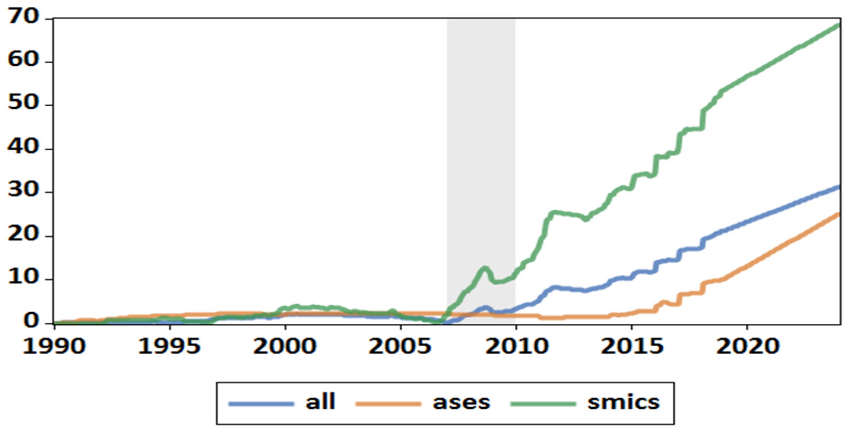
Real Gross Domestic Product at market prices	GDP	International Monetary Fund

below shows three policy variables that are used in this chapter: the macroprudential policy index, policy rates, and the common macroprudential policy index. The MPI is an overall measure of macroprudential policy actions taken in response to fluctuations in capital flows, credit, and asset prices (Cerutti et al., 2017). The MPI measures the intensity and direction of macroprudential policy actions. The MPI in its original form is given as a dummy variable. We transform each macroprudential policy index into a time series using the procedure by Kim and Mehrotra (2017). When MPI tightening (loosening) is undertaken, regardless of the measure or intensity, the level of the index increases (decreases) by one unit (Kim & Mehrotra, 2017). The new value is maintained until another action is taken. If two tightening measures are undertaken during the same month, and none in the direction of easing, the index level would increase by two units during that month (Bruno et al., 2015). In addition to the above, we aggregate macroprudential policy into two categories, one representing borrower-based tools and the other representing financer-based instruments along the lines of Cerutti et al. (2017) and Schoenmaker and Wierts (2011).

The study includes the policy rate because macroprudential measures are often taken with monetary policy measures (Galati & Moessner, 2018). This is reflected in the fact that macroprudential policy institutions combine monetary and prudential authorities. Moreover, monetary and macroprudential policies share similar transmission channels; consequently, employing one policy affects the other (Agénor & Pereira da Silva, 2022). Hence, it is important to distinguish monetary policy’s effects from macroprudential policy’s effects to prevent endogenous feedback between the two policies. The other explanatory variables used in the study are the VIX and Gross Domestic Product (GDP). GDP is used to capture the effects of the state of the economy (Gambacorta & Murcia, 2020). At the same time, the VIX is used to capture the effects of risk and uncertainty in global financial markets (Agrippino & Rey, 2021; Cerutti et al., 2017).

The study utilizes the CMPI as a proxy for macroprudential policy coordination. Unlike the MPI, which measures macroprudential policy activity within each individual member state, the CMPI captures the common components of policy actions across member states, thereby proxying situations in which policy coordination can occur. This measure is particularly useful for providing insights into the feasibility of cross-country macroprudential coordination, as effective coordination would require a relatively high degree of synchronization in macroprudential policy actions across jurisdictions.

The use of a coordinated macroprudential policy index as a proxy for policy coordination is grounded in both theoretical and practical considerations. From a theoretical standpoint, macroprudential policy actions are more likely to be uniform under coordinated frameworks than under purely national, self-oriented approaches (Korinek, 2017; Bianchi & Bengui, 2014). Evidence from the literature shows that the presence of supranational prudential authorities increases the relative weight assigned to financial stability objectives, compared to decentralized policymaking environments (Dell’Ariccia & Marquez, 2006). In addition, supranational oversight promotes convergence in macroprudential standards across jurisdictions, thereby reducing regulatory fragmentation (Acharya, 2009). In contrast, independent national authorities often pursue heterogeneous objectives or assign different weights to similar policy goals, resulting in divergence rather than alignment. A further explanation stems from the public good nature of financial stability. Macroprudential actions implemented in one country generate cross-border spillovers that benefit others. In the absence of coordination, this creates incentives for free riding, where some jurisdictions refrain from tightening policies in order to benefit from more stable capital flows generated elsewhere, without incurring the associated costs (Kara, 2016). Consequently, uncoordinated macroprudential policies tend to diverge rather than converge across countries. This provides a strong justification for employing the CMPI as a proxy for coordination and, importantly, for comparing its effects with those of the standard MPI, as any differential impact can be attributed to the role of policy coordination rather than policy stance alone.

A potential objection is that even in the absence of formal coordination, countries may still align their macroprudential policies by responding to common global factors such as the global financial cycle (GFC). However, empirical evidence indicates that countries exhibit heterogeneous responses to the GFC, undermining the notion of implicit coordination. Studies show that ASEs often adopt accommodative financial conditions during global upswings, generating capital flow surges that transmit to SMICS, where inflationary pressures are more pronounced (Bagliano & Morana, 2014; Bauer & Neely, 2014; Fratzscher et al., 2014; Aizenman et al., 2016; Tillmann, 2016). Further evidence suggests that SMICs typically deploy macroprudential policy defensively, as a buffer against external volatility, thereby requiring tighter policy stances (Ghosh et al., 2016), whereas in ASEs, such policies are more frequently used countercyclically to support credit expansion and output, implying relatively looser positions (Alam et al., 2019). This divergence reflects fundamentally different transmission mechanisms and policy objectives, meaning that even if macroprudential policy indices, the MPI in particular, are influenced by a common global driver, their responses are neither symmetric nor uniform across countries.

Another justification for the use of the CMPI is that the MPI of individual member states is unlikely to exhibit meaningful uniformity across countries, thereby limiting its usefulness as a proxy for macroprudential coordination. Although the MPI captures the frequency and intensity of macroprudential policy use, it does not adequately reflect cross-country comparability due to substantial heterogeneity in the design, calibration, and timing of instruments across jurisdictions as already detailed in Section 2.

This lack of uniformity across underlying policy instruments has important implications for an empirical analysis of macroprudential coordination. Since the MPI aggregates heterogeneous policy actions into a single frequency-based or intensity-based measure, it cannot distinguish between countries that implement similar numbers of policy changes but differ substantially in the nature, direction, and macro-financial context of those interventions. Consequently, cross-country differences in MPI values may reflect differences in domestic financial conditions and institutional preferences rather than genuine differences in policy alignment or coordination. This limitation motivates the use of the CMPI, which is designed to provide a more coherent and comparable measure of the overall macroprudential policy stance by consolidating diverse instruments into a unified index. In doing so, the CMPI offers a more suitable basis for assessing cross-country policy synchronization and potential coordination effects in macroprudential policy frameworks.

To construct the CMPI, the study employs principal component analysis (PCA), a statistical technique used to extract the shared variation from a set of correlated variables. In this context, country-specific macroprudential policy indices are likely to exhibit co-movement due to global financial cycles, shared regulatory standards, and coordinated policy responses. PCA allows this common component to be isolated and summarized into a single index, thereby providing an empirical proxy for cross-country macroprudential policy coordination (Jolliffe, 2002; Stock & Watson, 2002).

Let $X=(x_1,\cdots ,x_k)$ denote an $(n$ × $k)$ data matrix, where $n$ represents MPI observations for each country, and $k$ is the MPI variable for in each country. We estimate that the PCA is several steps. In the first step, the data are standardized to ensure comparability across variables using the Z-score: $Z_{ij}={\displaystyle \frac{x_{ij}-\overline{x_j}}{s_j}}$. This transformation produces variables with zero mean and unit variance, which prevents scale dominance in the subsequent analysis.

The Kaiser–Meyer–Olkin (KMO) Measure of Sampling Adequacy (MSA) evaluates whether the data are suitable for factor analysis or PCA by assessing the degree of common variance among variables relative to partial correlations. Formally, it compares the magnitude of observed correlation coefficients to the magnitude of partial correlations, with higher values indicating that the correlation structure is sufficiently compact to justify dimension reduction.

Table A1. Kaiser’s Measure of Sampling.

	MSA
BRA	0.864692
CHN	0.766329
GER	0.868233
IDS	0.96162
IND	0.90553
JAP	0.94626
MEX	0.837672
RUS	0.896429
TUR	0.879807
UK	0.920266
US	0.862391
ZAF	0.902463
Kaiser’s MSA	0.884037

displays the results. The overall KMO (Kaiser’s MSA) is 0.884, which falls within the “meritorious” range (0.80–0.89) according to Kaiser’s (1974) classification. This indicates that the dataset has a strong underlying common structure and is highly appropriate for PCA. In practical terms, it implies that the variables share a substantial proportion of common variance and that factor extraction will likely yield reliable and interpretable components.

At the country level, all individual MSA values exceed the commonly accepted minimum threshold of 0.50, with values ranging from 0.766 (China) to 0.962 (Indonesia). This suggests that each country contributes adequately to the overall factor structure, with no variable exhibiting weak sampling adequacy. Notably, Indonesia (0.962), Japan (0.946), and the United Kingdom (0.920) show particularly high MSA values, indicating strong shared variance with the rest of the system. Even the lowest value (China at 0.766) remains comfortably above the acceptable cutoff, confirming that no variable needs to be excluded on adequacy grounds.

Overall, the high KMO statistic (0.884), combined with uniformly strong individual MSAs, provides robust statistical justification for proceeding with PCA. It confirms that the correlation matrix is sufficiently factorable, and that the underlying data structure is well-suited for extracting a meaningful common component, such as the CMPI-based coordination factor used in this study.

The second step involves the construction of the variance-covariance matrix as $\mathrm{\Sigma }={\displaystyle \frac{1}{n-1}}{Z}^{\prime }Z,$ which captures the co-movement structure among the MPI variables.

Table A2. Covariance-variance matrix.

	BRA	CHN	DEU	IDS	IND	JAP	MEX	RUS	TUR	UK	US	ZAF
BRA	0.88	0.72	0.63	0.69	0.77	0.65	0.70	0.72	0.72	0.64	0.66	0.51
CHN	0.72	0.99	0.40	0.84	0.92	0.73	0.92	0.84	0.98	0.71	0.75	0.70
GER	0.63	0.40	0.96	0.72	0.51	0.86	0.64	0.74	0.47	0.87	0.81	0.79
IDS	0.69	0.84	0.72	0.98	0.77	0.92	0.97	0.98	0.90	0.94	0.96	0.93
IND	0.77	0.92	0.51	0.77	0.93	0.74	0.84	0.80	0.90	0.72	0.73	0.66
JAP	0.65	0.73	0.86	0.92	0.74	0.98	0.90	0.92	0.79	0.98	0.96	0.95
MEX	0.70	0.92	0.64	0.97	0.84	0.90	1.00	0.97	0.96	0.90	0.93	0.89
RUS	0.72	0.84	0.74	0.98	0.80	0.92	0.97	0.98	0.90	0.94	0.96	0.91
TUR	0.72	0.98	0.47	0.90	0.90	0.79	0.96	0.90	0.99	0.79	0.83	0.77
UK	0.64	0.71	0.87	0.94	0.72	0.98	0.90	0.94	0.79	0.99	0.97	0.97
US	0.66	0.75	0.81	0.96	0.73	0.96	0.93	0.96	0.83	0.97	0.98	0.94
ZAF	0.51	0.70	0.79	0.93	0.66	0.95	0.89	0.91	0.77	0.97	0.94	0.97

in the Appendix A displays the estimated variance–covariance matrix. The variance–covariance matrix indicates a strong degree of positive co-movement across all countries, with most off-diagonal values lying well above 0.60 and many exceeding 0.90. This suggests that macroprudential dynamics (as captured in the underlying data) are highly synchronized across both advanced systemic economies and systemic middle-income countries.

The strongest covariance relationships are observed among a core group of highly integrated economies, particularly IDN, Japan, the United Kingdom, the United States, Mexico, and Russia, where values frequently exceed 0.95, indicating near-complete co-movement. In contrast, relatively weaker linkages are observed for Germany with China (0.40) and Turkey (0.47), suggesting some degree of structural divergence from certain emerging market dynamics. The matrix points to a highly interconnected global system with limited segmentation, where macroprudential-related movements are largely driven by common global factors rather than country-specific shocks alone.

In the third step, we proceed by solving the eigenvalue problem $\mathrm{\Sigma }v=\lambda v$ where v denotes the eigenvector and $\lambda$ represents the corresponding eigenvalue. The eigenvectors define the directions of maximum variations in the data while the eigenvalues measure the amount of variance explained along each direction. These are ordered such that ${\lambda }_1\ge {\lambda }_2\cdots \ge {\lambda }_k$, with the component capturing the largest share of total variation, followed by orthogonal components explaining smaller shares. 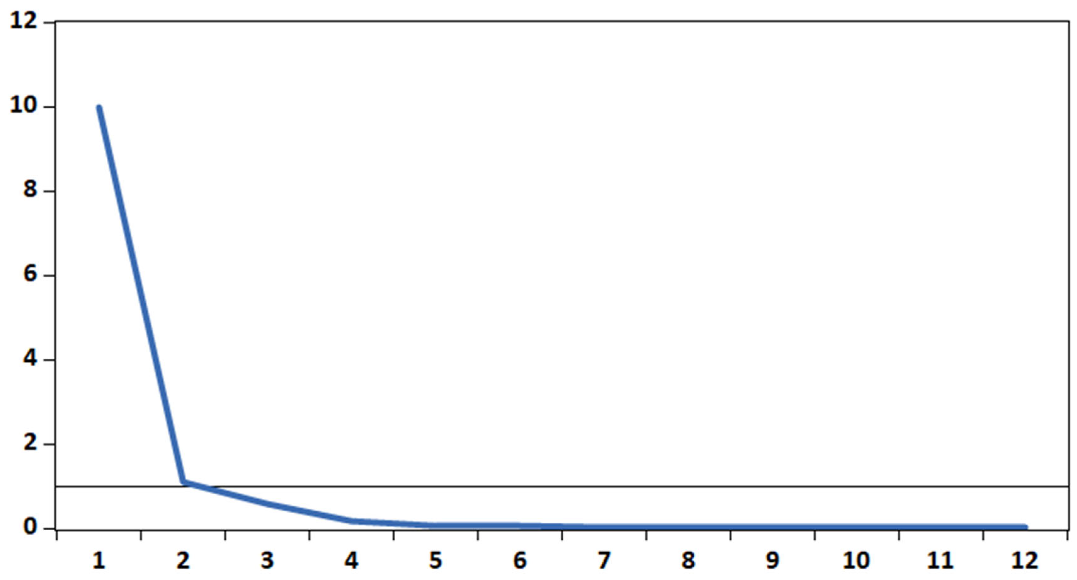Figure A1 displays the findings of this step using the scree-plot. The rule of thumb is to retain the number of components up to the point where the plot shows an “elbow,” after which the eigenvalues begin to level off. The scree plot shows a sharp decline in eigenvalues after the first component, with F1 explaining the dominant share of total variation (approximately 10 units). The second component has an eigenvalue slightly above the Kaiser threshold of 1, after which the curve flattens markedly, and additional components contribute negligible explanatory power. The clear “elbow” occurs at around the second principal component, indicating that a two-factor solution is sufficient to capture the meaningful structure in the data. Beyond this point, the remaining components largely reflect noise rather than systematic variation.

Fourth, we construct each principal component as a linear combination of the original variables, expressed as $PC=v{m}_1{x}_1+v{m}_2{x}_2\cdots v{m}_k{x}_k$ where $v{m}_j$ are the loadings associated with the $m$-th eigenvector. The resulting components are mutually orthogonal, ensuring that $Cov\left(P{C}_i, P{C}_j\right)=0$ for $i\ne j$. The component scores are then obtained by projecting the standardized data onto the eigenvector space. $F=ZV$ where $F$ is the matrix of principal component scores and V is the matrix of eigenvectors.

Table A3. Factor loadings.

	F1	F2	F3	F4	Communality	Uniqueness
BRA	0.72	0.19	0.59	0.23	0.95	0.05
CHN	1.00	0.00	0.00	0.00	1.00	0.00
GER	0.40	0.83	0.33	−0.07	0.97	0.03
IDS	0.84	0.50	−0.08	0.13	0.99	0.01
IND	0.92	0.07	0.23	−0.11	0.91	0.09
JAP	0.73	0.65	0.05	−0.13	0.98	0.02
MEX	0.92	0.36	−0.08	0.06	0.99	0.01
RUS	0.84	0.50	−0.01	0.13	0.97	0.03
TUR	0.98	0.13	−0.04	0.06	0.99	0.01
UK	0.71	0.69	0.01	−0.06	0.99	0.01
US	0.75	0.64	−0.02	0.08	0.98	0.02
ZAF	0.70	0.67	−0.16	−0.11	0.97	0.03

displays the loadings for each principal component. the PCA results suggest that macroprudential policy developments across countries are largely driven by a single dominant global factor (F1), reflected in consistently high loadings across both advanced and emerging economies. This indicates a strong common international component in macroprudential policy behavior, likely associated with shared regulatory standards, global financial cycles, or coordinated post-crisis reforms. A secondary factor (F2) captures additional cross-country heterogeneity, particularly among advanced economies such as the US, UK, Germany, and Japan, suggesting differences in policy intensity, institutional frameworks, or implementation depth. The remaining factors (F3 and F4) are negligible, indicating limited additional structure beyond these two dimensions. Overall, the MPI appears highly globally synchronized, with a strong common policy cycle and a weaker differentiation between country groups.

Turning to the question of how many factors to retain, the variance decomposition results provide strong evidence in favor of a single dominant factor (see

Table A4. Factor eigenvalues.

Factor	Variance	Cumulative	Difference	Proportion	Cumulative
F1	7.85	7.85	4.72	0.67	0.67
F2	3.13	10.98	2.58	0.27	0.94
F3	0.55	11.54	0.40	0.05	0.99
F4	0.15	11.69	---	0.01	1.00
Total	11.69	11.69		1.00

in the Appendix A). The first principal component (F1) explains 67% of the total variation in the macroprudential policy index (MPI) across countries, indicating a clearly dominant common factor. Although the second factor (F2) adds a further 27% of explanatory power, it mainly captures residual heterogeneity rather than an additional structural dimension, while F3 and F4 contribute only marginal gains (6% combined). The sharp decline in explained variance after F1, together with the clear “elbow” pattern in the decomposition, supports a parsimonious specification. Accordingly, retaining one factor is justified, with F1 serving as the common global macroprudential policy index and the remaining factors treated as minor idiosyncratic variations.

The use of PCA is particularly appropriate in this study for several reasons. First, it provides a data-driven method for dimensionality reduction, enabling the consolidation of multiple policy indicators into a single, tractable measure without imposing arbitrary weights. Second, it addresses potential multicollinearity among country-level policy variables, which could otherwise bias estimation results. Third, PCA has been widely used in macroeconomics and finance to construct composite indices and extract common factors, particularly in studies of financial cycles and global liquidity conditions (Bernanke et al., 2005; Kose et al., 2003).

Although, the CMPI is employed in this study as a proxy for cross-country macroprudential policy coordination, this interpretation requires careful qualification given its construction and informational content. While it captures cross-country co-movement in macroprudential policy actions, it does not directly observe coordination in a formal institutional sense, nor does it identify whether policy decisions are explicitly harmonized or jointly agreed. Instead, the index infers coordination indirectly through similarity in policy behavior, which may arise from common exposure to global financial cycles, parallel domestic shocks, or convergence in regulatory frameworks rather than deliberate policy alignment. Empirical findings based on the CMPI should therefore be interpreted as evidence of alignment or synchronization in macroprudential behavior rather than definitive proof of coordination. This distinction is crucial for correctly attributing cross-country policy dynamics and avoiding overstatement of the degree of institutional cooperation in macroprudential policymaking.

4.2. Econometric Specification and Estimation

The study employs the Dynamic Common Related Effects (DCCE) model to estimate the effects of macroprudential policies. The DCCE has several advantages over other methodologies. In contrast to the Mean Group (MG), the DCCE allows for the consistent estimation of a dynamic panel by adding lags of the cross-sectional means to account for the dependency of unobserved heterogeneity across units (Chudik & Pesaran, 2015). Moreover, it can constrain parameters to be homogenous across all units and support an unbalanced panel (Ditzen, 2018). Compared to the Pooled Mean Group (PMG), DCCE avoids maximum likelihood estimations, which can fit models including endogenous independent variables. Finally, the DCCE has an error-correction component, which is useful for distinguishing short-run parameters from long-run parameters and accounts for the speed of adjustment toward long-run equilibrium (Ditzen, 2018).

The study estimates the DCCE of Chudik and Pesaran (2015) and follows the estimation procedure of Ditzen (2018). In particular, the study estimates the impact of macroprudential policies using the following DCCE specification in the equation:

$$Y_{it}=\alpha Y_{i,t-1}+{\delta POL}_{it}+{\theta }_{vars}+{\displaystyle {\sum }_{P=0}^{P_T}}{\gamma }_{pol,ip}{\overline{POL}}_{t-p}+{\displaystyle {\sum }_{P=0}^{P_T}}{\gamma }_{vars,ip}{\overline{VARS}}_{t-p}+{\displaystyle {\sum }_{P=0}^{P_T}}{\gamma }_{y,ip}{\overline{Y}}_{t-p}+{\mu }_{it}$$

(1)

In Equation (1), Y refers to the dependent variable capital flows, $\alpha Y_{it-1}$ is the lags of the dependent variable, and $\delta {POL}_{it}$ refers to the impact of policy variables, $MPI, PR, and CMPI$, whereas and $\theta VAR{S}_{it}$ refers to other control variables: $CR, PP, and VIX$. Finally, $P_T$ represents the number of las included in cross-sectional averages.

Capital flows are chosen as the dependent variable in the DCCE because they are a key channel through which domestic and cross-border macroprudential policies transmit their effects, and they play a central role in global financial stability. Fluctuations in capital flows can amplify financial vulnerabilities in both advanced and emerging economies, as rapid inflows may fuel credit booms and asset price bubbles, while sudden outflows can trigger liquidity shortages and exchange rate volatility (Forbes & Warnock, 2012; Rey, 2015). Empirical studies have demonstrated that macroprudential policies, such as loan-to-value (LTV) or countercyclical capital buffers, are often targeted specifically at mitigating the risks associated with volatile capital flows (Cerutti et al., 2017; Lim et al., 2011). Furthermore, in a financially integrated environment, cross-country coordinated macroprudential policies can influence international capital movements, creating spillover effects that affect both the sending and receiving economies (Agénor & Pereira da Silva, 2022; Bénétrix et al., 2024). Given their systemic importance and sensitivity to both domestic and global regulatory actions, capital flows provide a comprehensive measure of the effectiveness and externalities of macroprudential policy, making them a natural and informative choice for the dependent variable in this analysis.

In this study, we employ the panel structural vector (PSVAR) methodology to estimate the transmission mechanism of macroprudential policy at a cross-country level. PSVAR models have been used extensively in both closed and open economies to evaluate monetary policy transmission mechanisms in a unified framework (Pedroni, 2013; Roch, 2019; Schmitt-Grohé & Uribe, 2018, for example). PSVAR generally has not been utilized to evaluate macroprudential policies. The only exception is Kim and Mehrotra (2017), who uses the PSVAR to analyze the effectiveness of macroprudential policies in the case of inflation-targeting Asian economies. The primary advantage of the PSVAR model lies in its ability to identify and recover structural shocks by imposing theoretically grounded restrictions on the estimated reduced-form VAR system. Unlike purely statistical models, PSVAR enables researchers to trace out the dynamic causal effects of shocks, such as those from macroprudential or monetary policy, on key financial and macroeconomic variables across countries or over time. The structural identification scheme, often based on economic theory (e.g., Cholesky decomposition, sign restrictions, or long-run restrictions), allows for the meaningful interpretation of impulse response functions and variance decompositions (Canova & Ciccarelli, 2013; Abrigo & Love, 2016).

In addition to this foundational strength, PSVAR models offer several other advantages. First, they are particularly well-suited for multi-country or panel settings, enabling the analysis of cross-sectional heterogeneity and dynamic interdependencies across economies. This is especially useful when investigating the potential spillover effects or synchronization of financial cycles and policy shocks across countries. The panel structure increases estimation efficiency by pooling information while still accounting for country-specific fixed effects or dynamics (Pedroni, 2013).

Second, PSVAR models allow for the incorporation of common global shocks and local idiosyncratic disturbances, making them an ideal framework for assessing the trade-offs or complementarities between self-oriented and coordinated macroprudential policies. By modeling the response of domestic variables to both domestic and foreign shocks, researchers can examine whether independent policy action suffices or if coordination yields superior outcomes in managing systemic risks.

Third, the PSVAR framework facilitates counterfactual simulations, which are essential for policy analysis. For example, researchers can simulate how financial conditions might have evolved in the absence of a specific policy intervention or under alternative coordination scenarios. These simulations offer valuable insights for designing optimal and responsive macroprudential policies in a globally interconnected financial system (Beetsma et al., 2019).

Consider the baseline model in Equation (2).

$$A_{i,0}{\left(L\right)x}_{i,t}=B_i\left(L\right)x+u_{i,t}$$

(2)

where $A_i\left(L\right)$ and $B_i\left(L\right)$ are the matrix polynomials in the lag operator $L,$ $u_{i,t}$ are the structural shocks, and $x_{i,t}$ is the vector of country-specific dimension $t=1,\dots , T$ for each member $i=1,\dots , M$ of the unbalanced panel, given by the following:

$$x_{i,t}=\left(\begin{array}{c}{CP}_{i,t}\\ {VIX}_{i,t}\\ {CR}_{i,t}\\ {HP}_{i,t}\\ GD{P}_{i,t}\\ {PR}_{i,t}\\ {MPI}_{i,t}\\ {CMPI}_{i,t}\end{array}\right)$$

(3)

Assuming that $A_{i}L$ is invertible, a reduced form PSVAR is estimated; afterwards, an identification scheme discussed below is imposed on the reduced identified structural shocks. Numerous identification schemes, such as structural factorization based on relevant economic theory, are usually employed (see Ngalawa & Viegi, 2011; Bernanke & Mihov, 1998; Sims, 1986; Bernanke & Gertler, 1986). Other studies employ zero long-run identification, known as the Blanchard–Quah long-run restrictions (Blanchard, 1989; Gali, 1999). Blanchard (1989) argues that imposing long-run restrictions offers more valid results since economic theory is generally concerned about the long run rather than the short run. Another approach is to use Sims (1986) recursive factorization based on the Cholesky decomposition of the matrix $A$. This identification scheme still uses economic theory to identify shocks. However, its main advantage is that it requires that the most endogenous variables are ordered last while exogenous variables are ordered first. This ensures that each variable responds to its most relevant shocks first. As a result, this approach is widely used in the literature (see Sims, 1986; Kim & Mehrotra, 2018; Christiano et al., 1999).

$$A=\left(\begin{array}{cccccccc}1& a_{12}& 0& 0& 0& a_{16}& 0& 0\\ a_{21}& 1& 0& 0& 0& 0& 0& 0\\ a_{31}& a_{32}& 1& a_{34}& a_{35}& a_{36}& a_{37}& a_{38}\\ a_{41}& a_{42}& a_{43}& 1& a_{45}& a_{46}& a_{47}& a_{48}\\ a_{51}& a_{52}& a_{53}& a_{54}& 1& 0& 0& 0\\ a_{61}& a_{62}& a_{63}& a_{64}& a_{65}& 1& 0& 0\\ a_{71}& a_{72}& a_{73}& a_{74}& a_{75}& a_{76}& 1& a_{78}\\ a_{81}& a_{82}& a_{83}& a_{84}& a_{85}& a_{86}& a_{87}& 1\end{array}\right)\ast B\left(\begin{array}{cccccccc}1& 0& 0& 0& 0& 0& 0& 0\\ 0& 1& 0& 0& 0& 0& 0& 0\\ 0& 0& 1& 0& 0& 0& 0& 0\\ 0& 0& 0& 1& 0& 0& 0& 0\\ 0& 0& 0& 0& 1& 0& 0& 0\\ 0& 0& 0& 0& 0& 1& 0& 0\\ 0& 0& 0& 0& 0& 0& 1& 0\\ 0& 0& 0& 0& 0& 0& 0& 1\end{array}\right)=u_{i,t}\left(\begin{array}{c}{CP}_{i,t}\\ {VIX}_{i,t}\\ {CR}_{i,t}\\ {HP}_{i,t}\\ {GDP}_{i,t}\\ {PR}_{i,t}\\ {MPI}_{i,t}\\ CMP{I}_{i,t}\end{array}\right)$$

(4)

This study follows Kim and Mehrotra (2017) by imposing a recursive factorization (Cholesky decomposition) on Equation (4) to identify structural shocks. The model consists of three target variables: capital flows (CP), credit (CR), and house prices (HP). Three policy instruments are included, namely the macroprudential policy index (MPI), the policy rate (PR), and the capital management policy index (CMPI). Furthermore, two additional explanatory variables are incorporated: Gross Domestic Product (GDP) and the Volatility Index (VIX). The identification strategy assumes that CP, CR, HP, GDP, and VIX contemporaneously affect CMPI, MPI, and PR, thereby allowing policymakers to observe current macro-financial conditions before adjusting policy instruments. This assumption is widely adopted in the structural VAR literature because policy authorities generally react to observed developments in financial and real sectors rather than to unobservable contemporaneous structural shocks (see Quint & Rabanal, 2013; Christiano et al., 1999). Similar recursive identification schemes have been used extensively in studies examining the interaction among monetary policy, macroprudential policy, and financial stability (Angelini et al., 2014; Bailliu et al., 2015; Kim & Mehrotra, 2017; Akinci & Olmstead-Rumsey, 2018). The use of a lower triangular matrix A and diagonal covariance matrix C is therefore theoretically and empirically grounded in the assumption that policymakers observe the contemporaneous state of the economy, while private-sector variables adjust more gradually because of information frictions, institutional rigidities, and policy transmission lags.

The first row implies that capital flows respond contemporaneously only to the VIX and monetary policy (PR). This restriction is motivated by both theory and empirical evidence regarding the determinants of global capital flows. The global financial cycle literature argues that international capital movements are largely driven by global risk conditions and monetary policy in major economies rather than by domestic macroeconomic fundamentals in the short run (Rey, 2015; Agrippino & Rey, 2021). In particular, increases in global risk aversion, proxied by the VIX, trigger portfolio rebalancing and sudden stops in emerging markets, while changes in monetary policy conditions influence global liquidity and investors’ search for yield (Bruno et al., 2015; Forbes & Warnock, 2012). Empirical evidence from Cerutti et al. (2017) further shows that capital flows are highly sensitive to global financial conditions and monetary policy shocks, especially in financially open emerging economies. The ordering therefore assumes that capital flows can react immediately to changes in global risk sentiment and monetary policy conditions because financial markets process such information rapidly. By contrast, other domestic variables are assumed to affect capital flows with a lag because portfolio allocation decisions are usually undertaken before domestic macroeconomic adjustments fully materialize.

The VIX is assumed to respond to all domestic variables only with a lag. This restriction is theoretically justified by the exogeneity of global financial conditions for small open economies. The VIX primarily reflects uncertainty and risk perceptions originating in advanced financial markets, particularly the United States, and is therefore commonly treated as an external variable in open-economy VAR models (Rey, 2015; Bekaert et al., 2013). Since the economies examined in this study are insufficiently large to contemporaneously influence global volatility conditions, domestic macro-financial developments are unlikely to affect the VIX within the same period. Similar assumptions have been employed in empirical studies examining spillovers from global financial conditions to emerging markets (Bruno et al., 2015; Agrippino & Rey, 2021).

GDP is assumed to respond contemporaneously to CP, VIX, CR, and HP, but only with a lag to policy variables. This restriction reflects the sluggish adjustment of real economic activity to policy interventions due to implementation delays, information rigidities, habit persistence, and investment planning horizons. According to Ngalawa and Viegi (2011), changes in policy stances typically require time before households and firms revise spending, production, and investment decisions. This view is consistent with the traditional monetary-transmission -mechanism literature, which documents that monetary policy affects output with “long and variable lags” (Friedman, 1961; Christiano et al., 1999). However, GDP is allowed to react contemporaneously to credit and house prices because financial conditions directly affect consumption, investment, and aggregate demand through wealth and balance-sheet channels. The financial accelerator framework developed by Bernanke et al. (1999) suggests that changes in credit conditions and asset prices immediately influence borrowing capacity and investment behavior. Similarly, the housing wealth literature demonstrates that rising house prices stimulate household consumption through collateral and wealth effects (Iacoviello, 2005). Empirically, Gomez-Gonzalez et al. (2015) establish strong bidirectional Granger causality between financial variables and real economic activity, supporting the assumption of contemporaneous interactions among GDP, credit, and house prices.

Credit is assumed to respond contemporaneously to all shocks because financial intermediaries and borrowers react rapidly to changes in economic and financial conditions. Credit markets are inherently forward-looking, and lending decisions incorporate contemporaneous information about output, risk, interest rates, and asset prices. According to Agénor and Pereira da Silva (2022), credit serves both consumption-smoothing and investment-financing functions, making it highly responsive to macroeconomic and financial shocks. This assumption is also consistent with the bank lending channel literature, which shows that changes in monetary and financial conditions quickly influence bank balance sheets and loan supply (Bernanke & Blinder, 1988). House prices are similarly assumed to respond contemporaneously to all shocks because property markets rapidly incorporate information regarding credit conditions, income expectations, and financial sentiment. Empirical studies have consistently documented strong contemporaneous interactions among house prices, credit growth, and macroeconomic conditions (Iacoviello & Neri, 2010; Akinci & Olmstead-Rumsey, 2018).

Macroprudential policy and monetary policy are treated as endogenous to all variables in the system. This restriction is consistent with the growing consensus that policymakers adjust policy instruments after observing developments in financial markets, credit growth, inflation, and real economic activity. Existing studies such as Kim and Mehrotra (2017), Quint and Rabanal (2013), Angelini et al. (2014), and Bailliu et al. (2015) employ similar assumptions, arguing that policy authorities systematically react to macro-financial conditions to mitigate systemic risk and stabilize the economy. Theoretical DSGE models incorporating financial frictions likewise assume that central banks and macroprudential authorities observe the state of the economy before implementing policy responses. Furthermore, the policy reaction function literature emphasizes that both monetary and macroprudential authorities operate in a countercyclical manner, tightening policy during periods of excessive credit growth and financial overheating while easing during downturns (Taylor, 1993; Galati & Moessner, 2013).

Finally, the identification scheme assumes that monetary policy does not contemporaneously respond to macroprudential policy shocks, whereas macroprudential policy responds contemporaneously to monetary policy shocks. This restriction reflects the institutional hierarchy and coordination structure commonly observed between monetary and macroprudential authorities. Monetary policy decisions are generally implemented by central banks with established mandates and regular policy schedules, while macroprudential authorities frequently adjust their policy stance in response to prevailing monetary conditions and financial imbalances (Libich, 2020). Theoretical contributions suggest that macroprudential policy often complements monetary policy by counteracting financial vulnerabilities created by accommodative interest-rate environments (Angelini et al., 2014; Beau et al., 2012). Empirically, studies have found that macroprudential tools are frequently tightened following expansionary monetary policy episodes to curb excessive leverage and risk-taking (Bruno et al., 2015; Kim & Mehrotra, 2017). The recursive ordering adopted in this study therefore reflects both institutional realities and the empirical evidence on the interaction between monetary and macroprudential policy frameworks.

5. Results and Discussion

The objective of study is to examine the effectiveness of macroprudential policies in ASEs and SMICs. This section presents the findings of the study.

5.1. Preliminary Analysis

Table 2. Descriptive statistics of macroprudential, real, and financial variables; source: STATA-19 estimates.

	Mean	Median	Minimum	Maximum	Std. Dev.
CAP	7.74	7.99	−1.04	12.17	2.33
CR	88.77	113.60	0.00	214.02	54.36
HP	73.05	93.76	0.00	189.45	102.61
MPI	3.18	0.00	−11.00	69.00	10.49
GDP	4.43	4.61	0.00	4.68	0.89
CMPI	137.65	124.00	1.00	225.00	102.61
PR	7.02	5.00	−3.00	210.00	16.28
VIX	19.67	17.77	10.12	62.67	7.59

below reports the descriptive statistics. A large variation is found for our explanatory variables. For instance, capital flows range from −1.04% to 12.1%, with a standard deviation of 2.33 and a mean of 7.74%. Credit ranges from zero percent to 214.02% of GDP, with a standard deviation of 54.36 and a mean of 88.77% of GDP. On the other hand, house prices range from zero percent to 189.45, with a standard deviation of 102.61 and a mean of 73.05. The range statistics suggest that there is more variation in credit compared to house prices and capital flows. Moreover, house price variations are larger than capital flow variations. The standard deviation statistics suggest that house price variations are more volatile, followed by credit variations, and capital flows have the least volatile changes.

Table 2 also reports large variations in the policy variables. The MPI ranges from −11% to 69%, with a standard deviation of 10.49 and a mean of 3.18. The policy rate, on the other hand, ranges from −3 to 3,555,085.8 basis points. The standard deviation is 5718, and the mean is 154.18 basis points. The range and standard deviations show that monetary policy fluctuations are larger than those of macroprudential policies. This is because while monetary policy decisions can be easily taken, macroprudential policy faces problems of political lobbying. This means that there are many stakeholders, each with a different objective, seeking to influence macroprudential policy decisions. Harmonizing these objectives results in delaying taking macroprudential policy actions or implementing an action once it has been agreed upon. Ultimately, this means that macroprudential policy is slow to change compared to monetary policy.

After the descriptive statistics, the study conducted cross-sectional, unit root, and cointegration tests to determine the suitability of our variables for the DCCE. Due to the nature of macroeconomic variables and panel data, there are increasing chances that cross-sectional dependence may prevail. As a result, tests should be conducted to verify its presence to address it when estimating the DCCE. To this effect, the following tests, Pesaran (2021)—CD, Pesaran (2021)—scaled LM, and Pesaran (2021)—Friedman, are conducted to detect the presence of cross-sectional dependency. According to Ali et al. (2022), the findings of these tests are crucial not only for deciding on an estimation technique but also to determine the suitability of employing first-generation unit roots tests, which assume cross-sectional independence against second general unit roots tests (Pesaran, 2007), which consider cross-sectional dependency. The null hypothesis of the above tests is the absence of cross-sectional dependence. The alternative hypothesis is that cross-sectional dependency exists.

Table 3. Cross-sectional dependency; source: STATA-19 estimates; notes: ** and *** are p-values corresponding to the 95th and 99th level of significance, respectively.

	Pesaran CD	Pesaran Freidman	Pesaran Scaled LM
CAP	29.42 ***	234.76 ***	234.73 **
CR	6.15 ***	1379.66 ***	11,543.85 ***
PP	6.15 ***	433.2 ***	147.81 ***
MPI	54.92 ***	1656.47 ***	736.01 ***
GDP	54.61 ***	1849.76 ***	369.32 ***
CMPI	94.18 ***	1580.12 ***	847.75 ***
PR	106.08 ***	2176.62 ***	706.40 ***
VIX	111.05 ***	3465.12 ***	144.00 ***

displays that the parameters of the Pesaran (2021)—CD, Pesaran (2021)—scaled LM, and Pesaran—Friedman tests are statistically significant at all levels. Therefore, the null hypothesis of no cross-sectional dependency is rejected.

Consequently, the study accepts some degree of cross-sectional dependency in our variables. This may arise from several factors, including common shocks and unobserved components in the error terms, spatial dependency, and idiosyncratic pairwise dependency in the disturbances with no pattern of common components or spatial dependency (Robertson & Symons, 2000; Pesaran, 2021; Anselin, 2001). Over the past three decades, ASEs and SMICs have become increasingly financially and economically integrated, which implies that the interdependence of cross-sectional units has also increased between these economies (De Hoyos & Sarafidis, 2006). Consistent with this, there is substantial evidence to show that share prices and house prices are driven by common global factors between these economies (Rey, 2015).

The findings of the cross-sectional dependency suggest that second-generation unit root tests should be employed. However, first- and second-generation unit roots tests are conducted to avoid misleading results. To this effect, Levin, Lin, and Chu (LLC), Hadri-LM, and the Pesaran CADF (PESCADF) are employed in this study.

Table 4. First- and second-generation unit roots; source: STATA-19 estimates; notes: *, **, and *** are p-values corresponding to the 90th, 95th, and 99th level of significance, respectively.

	LLC		HADRI		PESCADF
	Level	1st Diff	Level	1st Diff	Level	1st Diff
CAP	0.00	−29.34 ***	178.93 ***	−2.17	2.16 *	−6.19 ***
CR	−1.26	−30.24 ***	609.74 **	−1.10	−2.68 ***	−6.18 ***
PP	2.46	−9.63 ***	92.34 ***	−1.76	−1.55	5.68 ***
MPI	15.60	−23.57 ***	615.32 ***	29.42	−0.80	−6.19 ***
GDP	5.10	−4.73 ***	246.29 ***	4.64	−2.81 ***	−5.37 ***
CMPI	−4.37 ***	−4.37 ***	144.42 ***	−3.50	−3.74 ***	−6.11 ***
PR	−0.57	64.04 ***	13.74 ***	−3.49	−1.99	−5.39 ***
VIX	−0.54	77.56 ***	34.32 ***	−1.53	−2.29	8.33 ***

below reports the findings. The LLC is a first-generation unit roots test that tests the null hypothesis of non-stationarity against the alternative hypothesis of stationarity. The parameters of the LLC at the level are statistically insignificant except for the variables TIGHT which are significant at all levels. Therefore, the study fails to reject the null hypothesis of non-stationarity at a level for most variables. However, when we take the first difference of all variables, then the parameters of the LLC are now significant at all levels. Consequently, the study rejects the null hypothesis of non-stationarity for all variables at first difference. The LLC is a classical unit root test with limited power to reject the null hypothesis and does not account for cross-sectional dependency. Consequently, to bridge the first gap, which is the limited power to reject the null hypothesis, the Hadri-LM test is used to corroborate the findings of the LLCs.

The Hadri–LM tests the null hypothesis of stationarity against the alternative hypothesis of non-stationarity. At the level, the parameters of the Hadri-LM test are statistically significant at all levels. Therefore, the study fails to reject the null hypothesis of stationarity and accepts that all the variables are not stationary at the level. However, at the first difference, all parameters of the Hadri-LM are statistically insignificant. Hence, the study fails to reject the null hypothesis and accepts that all variables are stationary at the first difference. As noted earlier, first-generation unit roots tests such as the LLC do not consider cross-sectional dependency between variables. Considering this, the second-generation unit root test of Pesaran CDAF is conducted to cross-check the findings of the first-generation unit root tests. The parameters of PESCADF are statistically significant at all levels at first difference. Therefore, the null hypothesis of non-stationarity is rejected, and the study accepts that the variables are stationary at first difference. Consequently, to estimate the DCCE, we will take the first difference of all variables given the congruency of the unit root tests that all variables are only stationary at the first difference.

Before estimating the DCCE, the study conducts several cointegration tests to ascertain the presence of long-run relationships. To achieve this, the Westerlund (2007) cointegration test is employed. Westerlund (2007) accounts for cross-sectional dependency.

Table 5. Westerlund cointegration test; source: STATA-19 estimates.

Statistic	Value	Z-Value	p-Value
Gt	−0.183	6.861	0.000
Ga	−1.031	4.824	0.000
Pt	1.024	6.171	0.000
Pa	0.626	3.771	0.000

below displays the results. Gt and Ga tests the null hypothesis of no cointegration in at least one cross-sectional unit. The p-values suggest that the null hypothesis is rejected at all levels of significance. The rejection of the null hypothesis provides evidence of cointegration for at least one cross-sectional unit. The Pt and Pa test statistics pool information over all the cross-sectional units to test the null hypothesis of no cointegration in the whole panel. Given the p-values in Table 5, the study rejects the null hypothesis and accepts that there is evidence cointegration for the whole panel.

5.2. DCCE Results

Table 6. Dynamic common correlated effects model results; source: STATA-19 estimates; notes: *, **, and *** are p-values corresponding to the 90th, 95th, and 99th level of significance, respectively.

	ALL	ASES	SMICS
EC	−0.13 ***	−0.12 ***	−0.10 ***
	(−7.18)	(−23.37)	(−5.05)
MPI	−0.78 ***	−0.20	−0.89 **
	(−3.56)	(−1.19)	(−2.67)
	(−1.50)	(−1.49)	(−0.94)
GDP	−0.48 *	−0.50 *	−0.81 *
	(−1.19)	(−0.17)	(−0.13)
VIX	−0.54 *	−0.70 *	−0.07 *
	(−0.14)	(−0.33)	(−0.25)
CR	0.03 **	0.04 ***	0.02 **
	(−1.76)	(−0.69)	(−1.08)
	(−0.15)	(−1.44)	(−0.25)
HP	0.12	0.43	0.22
	(−0.11)	(−0.19)	(−0.14)
PR	0.03 *	0.11 *	0.21 *
	(−0.89)	(−1.95)	(−1.91)
CMPI	−0.48 ***	−0.63 **	0.98 *
	(−0.07)	(−0.11)	(0.21)

presents the first results of the DCCE. In the DCCE, the dependent variable is capital flows. The other two target variables, CR and HP, are used as explanatory variables for now. In relation to capital flows, the aim of macroprudential policy measures is to regulate or restrict cross-border movements of capital (inflows and outflows of financial assets). The core aim is to manage the risks associated with volatile international capital flows and to preserve macroeconomic and financial stability. First, consider the EC terms. The term has a negative sign, suggesting the existence of a long-run relationship between macroprudential policies and capital flows. This indicates that both domestic and common macroprudential policies, MPI and CMPI, have a cross-country effect. Thus, both policy types can be considered when regulating capital flows.

At the aggregate level, the estimated coefficient on the macroprudential policy index indicates that a one percentage point increase in macroprudential intensity reduces capital flows by approximately 78 percent on average, ceteris paribus. This result is consistent with the theoretical prediction that tighter macroprudential regulation constrains credit creation, reduces leverage, and thereby weakens cross-border capital inflows through the bank lending and risk-taking channels (Borio et al., 2014; Bruno et al., 2015). In the global financial cycle framework, macroprudential tightening operates by increasing balance sheet constraints on financial intermediaries, which in turn limits their capacity to intermediate international capital flows (Rey, 2015). The negative and economically large aggregate effect therefore aligns with models in which macroprudential policy acts as a binding constraint on the expansion of externally financed credit booms, particularly in financially integrated economies (Osina, 2021; Eller et al., 2021).

However, important heterogeneity emerges across country groups. The MPI coefficient is negative but statistically insignificant in advanced systemic economies, whereas it is negative, larger in magnitude, and statistically significant at the five percent level in systemic middle-income countries. This pattern is consistent with the empirical literature showing that macroprudential policy is more binding and more effective in emerging and middle-income economies, where financial frictions are higher and regulatory arbitrage is more limited by institutional depth (Cerutti et al., 2017; Akinci & Olmstead-Rumsey, 2018). In contrast, ASEs typically exhibit deeper financial markets, greater capital account openness, and more sophisticated financial instruments, which allow capital flows to adjust around macroprudential constraints. As a result, self-oriented macroprudential policies in ASEs tend to operate more through composition and risk-shifting effects rather than through outright reductions in aggregate capital inflows. For instance, Baskaya et al. (2024) found that the effectiveness of macroprudential policy in containing capital flows fades if a country has a large financial system.

From a policy perspective, this asymmetry implies that self-oriented macroprudential frameworks are more effective in SMICs as a countercyclical stabilization tool for capital flows, while in ASEs, their impact is partially diluted by a higher degree of financial development. This implication supports the view that domestic macroprudential autonomy is structurally constrained in core financial centers, reinforcing the relevance of spillovers from global financial conditions in these economies (Rey, 2015; Forbes & Warnock, 2012).

Turning to common macroprudential policy, the coefficient on the common macroprudential policy index, the estimates are negative and statistically significant across all samples, with magnitudes of −0.48 for the full sample, −0.63 for ASEs, and −0.98 for SMICs. This indicates that synchronized macroprudential actions exert a stronger contractionary effect on capital flows than the MPI, particularly in SMICs.

The DCCE results of the CMPI are consistent with the view that synchronized macroprudential tightening exerts a statistically significant contractionary effect on capital flows across economies. The estimates remain negative and robust across all samples, with magnitudes of −0.48 for the full sample, −0.63 for ASEs, and −0.98 for SMICs, indicating that the effect intensifies in more financially constrained and structurally vulnerable economies. This pattern is consistent with a dominant credit-supply channel operating under coordinated policy regimes, whereby the simultaneous tightening of macroprudential standards raises borrowing costs and restricts credit availability across jurisdictions, thereby amplifying the reduction in cross-border financial activity. The stronger response in SMICs suggests heightened sensitivity to global financial tightening and greater dependence on external financing, which makes capital flows more responsive to changes in financial conditions. In contrast, ASEs exhibit a comparatively muted response, reflecting deeper financial markets and greater absorptive capacity in the face of tighter macroprudential environments. Overall, the DCCE findings reinforce the interpretation that synchronized macroprudential policy may enhance systemic stability, doing so at the cost of reducing capital flow dynamics, with heterogeneous effects driven by structural differences across economies.

In contrast to the MPI, common macroprudential actions are more effective across all country groups, suggesting that policy coordination enhances the stabilization of global capital flows. However, this also implies a potential cost in terms of reduced financial integration efficiency, as coordinated tightening constrains cross-border risk sharing and may intensify global liquidity shortages during synchronized regulatory cycles.

The parameters of PR are positive and statistically significant at the 1 percent level. They are 0.03, 0.11, and 0.21 for ALL ASEs and SMICs. This means that monetary policy has a significant expansionary effect on capital flows. Tightening monetary policy increases capital flows. However, when comparing the parameters of PR to MPI, MPI parameters have a large magnitude, indicating that macroprudential policy has a more substantial impact. The parameters for GDP are −0.48, −0.50, and −0.81 for ALL, ASES, and SMICs, respectively. The parameters on VIX are −0.54, −0.70, and −0.07, respectively. This demonstrates that GDP and the VIX have a dampening effect on cross-country lending. This is significant at the ten percent level.

A key caveat in interpreting the DCCE results is that the estimates are presented within a pooled framework, despite the sample comprising economies that differ in income levels, financial depth, and institutional structures. At first glance, this raise concerns that average coefficients may mask meaningful heterogeneity in macro-financial responses across countries. However, this concern is partially mitigated by the fact that the sample is not randomly heterogeneous: the ASE group (United States, United Kingdom, Germany, and Japan) consists of advanced, highly integrated, and financially deep economies with liberalized capital accounts and globally systemically important financial institutions, while the SMIC group (Brazil, China, India, Indonesia, Russia, Mexico, Turkey, and South Africa) comprises large emerging markets that, despite institutional differences, share common features such as greater exposure to external financing cycles, higher sensitivity to global risk conditions, and more pronounced macro-financial frictions. In this sense, the grouping reflects economically meaningful similarities in financial openness and global financial cycle sensitivity, which justifies a pooled interpretation with caution rather than the rejection of aggregation altogether.

Moreover, DCCE explicitly addresses concerns related to heterogeneity and cross-sectional dependence (Pesaran, 2007; Chudik & Pesaran, 2015). It allows slope coefficients to vary across countries while controlling for unobserved common factors, such as global liquidity conditions, risk appetite, and international financial cycles, that simultaneously influence all cross-sectional units. This is achieved by augmenting the regression with cross-sectional averages of both dependent and explanatory variables, which serve as proxies for these unobserved global shocks. As a result, the estimator effectively separates country-specific responses from common global influences, ensuring that the estimated effects are not biased by omitted common factors. In this way, the DCCE framework is well suited to panels such as ASEs and SMICs, where heterogeneity exists but is structured and jointly driven by shared exposure to global financial conditions.

5.3. PSVAR Results

In this section, the findings of the panel structural vector autoregression (PSVAR) are presented. The Cholesky decomposition was employed to identify structural shocks and responses. This means that the most exogenous variables, VIX and CAP, were ordered first, whereas the most endogenous variables, PR, MPI, and CMPI, were ordered last. Figure 2 plots the impulse response functions of the three target variables to shocks, i.e., CAP, CR, and HP.

The solid blue lines represent all impulse response functions, while the dashed blue lines are 95 percent confidence intervals. The x-axis is measured in months and extends to 4 years, while the y-axis is percentage changes. Firstly, the study notes the responses of CAP, CR, and HP to the most endogenous shocks, CMPI and MPI. Shocks to CMPI and MPI trigger significant responses across the target variables, and their interpretation requires a clear distinction between the short-run dynamics captured by the panel SVAR (Cholesky identification) and the long-run relationships estimated using the DCCE framework. The SVAR results reflect contemporaneous and short-horizon adjustments, whereas the DCCE estimates capture equilibrium responses after common global factors and dynamic adjustments have fully materialized. Figure 2 shows that following a common macroprudential policy shock, CMPI, CAP, CR, and HP all increase on impact.

This short-run expansionary response can be understood through the volatility channel, particularly as captured by the VIX. A coordinated tightening of macroprudential policy can reduce perceived systemic fragility and lower global uncertainty, thereby compressing volatility premia. In line with this channel, lower volatility improves investor confidence and reduces uncertainty in cross-border financial markets, which can temporarily encourage capital inflows and financial intermediation despite tighter regulatory conditions. This explains why CAP and CR may initially rise following the shock, as reduced volatility dominates the immediate credit-constraining effects. However, these results should be interpreted with caution. While the short-run increase in capital flows and credit may reflect improved market confidence, stronger financial intermediation, and more favorable financing conditions, sustained periods of compressed volatility and abundant liquidity may also encourage excessive risk-taking and leverage accumulation.

At the same time, the increase in house prices is consistent with this risk-compression mechanism, as lower-volatility environments tend to strengthen risk appetite and collateral valuations, reinforcing short-run credit expansion through balance sheet effects. This suggests that the volatility channel operates alongside, and in the short run may outweigh, the direct regulatory tightening channel. Nevertheless, rising house prices and expanding credit conditions may also signal the build-up of financial vulnerabilities if asset valuations become disconnected from underlying fundamentals. Since the present analysis does not directly test whether these developments are sustainable or indicative of speculative behavior, no definitive conclusions can be drawn regarding the emergence of asset price bubbles. The findings therefore imply that policymakers should carefully consider the potential adverse effects of stimulatory financial conditions and balance short-run market stabilization objectives against longer-run financial stability risks.

Importantly, these short-run dynamics do not contradict the earlier DCCE findings. Instead, they complement them. The DCCE results capture the long-run contractionary effect of synchronized macroprudential policy on capital flows, driven by sustained increases in borrowing costs and tighter balance sheet constraints. In contrast, the SVAR results highlight that in the short run, adjustment frictions, expectations, and portfolio rebalancing can generate expansionary or non-linear responses. Taken together, the two approaches suggest a coherent narrative: macroprudential shocks may initially trigger adjustment-driven expansions in credit and capital flows, but over time, the dominant long-run effect is contractionary, as captured in the DCCE estimates.

Following a shock to the MPI, CAP reacted by increasing, but CR and HP reacted by falling. This suggests that a domestic macroprudential policy shock raises capital flows but reduces domestic credit and house prices. The effect of the MPI on CAP can be associated with the ‘reallocation effects’ of macro-prudential policies. When a domestic policymaker enacts a macroprudential policy measure, the financial institutions in the jurisdiction where the measure is enacted can face higher regulatory constraints (Kang et al., 2017). As a result, they may not be able to continue their activities as before (Bengui & Bianchi, 2014). Those financial institutions with a global presence will circumvent the regulation by shifting their activities to jurisdictions with less strict regulations (Houston et al., 2012). This will result in high financial flows in the recipient jurisdictions. Hence, a shock to the MPI can be associated with increased capital flows. Similar findings were obtained by Cerutti et al. (2017), Houston et al. (2012), Buch and Goldberg (2016), and Akinci and Olmstead-Rumsey (2018).

This mechanism can be further interpreted within the broader context of macroprudential policy as a quasi-public good in global finance. Because macroprudential tightening in one jurisdiction reduces systemic risk and volatility spillovers internationally, it generates positive externalities for other economies, which may therefore have reduced incentives to implement equally stringent measures. This strategic interaction can lead to a globally suboptimal level of macroprudential coordination, allowing regulatory arbitrage and the cross-border reallocation of financial activity to persist. In this setting, capital flows increase not only because of direct substitution effects by global banks, but also because differences in regulatory intensity across countries remain sufficiently large to sustain arbitrage opportunities. In contrast to CAP, Figure 2 shows that an MPI shock has a contractionary effect on CR and HP. This is because tightening domestic macroprudential policies increases the cost of borrowing and lending, causing credit to decline (Kim & Mehrotra, 2017). As credit declines, there is less spending on housing; as a result, pressure on asset prices is reduced, causing them to decline (Carreras et al., 2016; Demertzis & Agur, 2018).

Next, we turn to the responses of the target variables to GDP and PR. Figure 2 shows that CAP, CR, and HP respond to GDP and PR shocks. Following a shock to PR, CAP responded by rising. This proves that a monetary policy shock has an expansionary effect on capital flows. This suggests that capital flows are sensitive to monetary policy shocks (Rey, 2015; Agrippino & Rey, 2021; Claessens, 2013) but the increase in credit is statistically insignificant, whereas the increase in HP is statistically significant (see Figure 2). The impact of the PR on HP can be linked to what has been termed the ‘price puzzle’, an occurrence where the tightening monetary policy results in higher prices (Bernanke & Mihov, 1997). Several explanations exist for the prize puzzle. For instance, if policymakers increase interest rates because they anticipate that prices will overheat, but the increase in the interest rates is not enough to cool down prices, in that case, tight monetary policy will coincide with a rise in the prices (Sims, 1992). Alternatively, if policymakers react with a delay to a price shock, prices will already be higher by the time they tighten policies (Sims, 1992).

Figure 2 shows that HP and CR responded by increasing following a GDP shock CAP. However, the responses of CAP and HP are not statistically significant, whereas the response of CR is statistically significant at the 95 percent confidence interval. This finding suggests that domestic credit is more sensitive to economic changes than capital flows and house prices. Next, the study considers the responses of the target variables to exogenous shocks. Figure 2 displays the responses of CAP, CR, and HP to the VIX. CAP and CR HP responded to VIX shocks. Following a VIX shock CAP and HP responded by falling. Similar findings were obtained elsewhere. For instance, Rey (2015) found that around a crisis time, the VIX rises, indicating high risk and uncertainty in financial markets; in turn, markets reduce their activity as a precaution. Agrippino and Rey (2021) found that there is a negative relationship between the VIX capital flows and asset prices. These findings help justify why following a shock to the VIX, CAP, and HP responded by declining. On the other hand, CR reacted by increasing following a VIX shock, but the response is statistically insignificant.

After discussing the responses of target variables to endogenous and exogenous variables, we next turn to discuss the interactions between the target variables. First, let us consider the effects of CAP on CR and HP. Following a shock to capital flows, CR and HP reacted by falling. This provides evidence that capital flows harm credit and house prices. This is because capital flows are considered to be procyclical and volatile as they obey unstable global factors such as the VIX (Rey, 2015). As a result, capital flows may be inappropriate for the financial conditions of many economies. They may lead to excessive credit growth during good times and excessive retrenchment in bad times (Rey, 2015). The literature shows that excessive growth in credit and house prices is a good recipe for financial distress (Gourinchas & Obstfeld, 2012; Schularick & Taylor, 2012). Hence, CAP harms CR and HP. Second, following a shock in CR and HP, CAP increased. When domestic markets are booming, agents will also increase their financial activities abroad, resulting in higher capital flows. The study found that the response of HP to CR is insignificant, meaning the housing market is less sensitive to changes in the credit market (see Figure 2). Likewise, the response of CR to HP is not significant.

After discussing the responses of target variables to shocks, the section discusses the responses of policy variables to shocks. Figure 3 plots the impulse-response functions of PR, MPI, and CMPI to shocks. The solid blue lines are the impulse-response functions, whereas the dashed blue lines are the 95 percent confidence intervals. The x-axis is measured in months, whereas the y-axis is the percentage changes. First, let us consider the responses of PR, MPI, and CMPI to target variables. Following a CAP shock, the MPI and CMPI reacted by increasing (see Figure 3). However, the responses are not statistically significant. This finding indicates that macroprudential policies are less sensitive to changes in capital flows. Following a CR and HP shocks, the MPI reacted by rising, but the CMPI reacted by declining. This finding suggests that domestic macroprudential policy tighten in response to credit and house price shocks, but common macroprudential policies are loosened in response to credit and price shocks. The response of the CMPI reflects common endeavors to stimulate growth in the housing and credit markets. However, the response of the MPI reflects domestic endeavors to slow down excessive credit and house price growth in order to promote domestic financial stability (Galati & Moessner, 2013).

Figure 3 suggests that the PR responds to CAP, CR, and HP shocks. According to the figure, the PR responds by rising following a CAP shock, but this is not significant. However, when the CR is disturbed, the PR rises significantly. This suggests that monetary policy is tightened following a credit shock. The response of the PR to a credit shock can be associated with the ‘lean against the wind’ view on monetary policy and financial stability. In this view, monetary policy has an active role in containing credit shocks since they may induce inflation through their stimulatory effects on income and spending, thereby affecting the price stability objective. In response to an HP shock, monetary policies are loosened. This can help explain the prize puzzle observed above. Relaxing monetary policy following an HP can stimulate the housing market, which means that more spending on housing puts upward pressure on house prices.

Next, the study discusses the response of policy variables to the VIX and GDP. Following a shock to the VIX, the MPI and CMPI reacted by declining. However, their responses are not statistically significant. In contrast, following a VIX shock, the PR rises, and the response is statistically significant at the 95 percent confidence interval. The policy responses to the VIX shocks suggest that macroprudential policies are not sensitive to changes to the VIX, but monetary policy is. Hence, monetary policy can be used to stabilize economies after an exogenous VIX shock. Following a GDP shock, both the MPI and PR reacted by falling. However, the fall in the PR is not significant. This suggests that domestic macroprudential policies are more sensitive to economic activity than monetary policy. Thus, domestic macroprudential policies can also be used to deal with developments in the real economy (see Angelini et al., 2014; Liu & Molise, 2020). In contrast, to the MPI and PR, the CMPI reacted to a GDP shock by rising. This finding suggests that common macroprudential policies can be used to stabilize real economic activity in order to achieve output stability.

The findings of this section presented above have significant crucial implications for the transmission mechanism of macroprudential policies. First, it was found that the MPI reacts significantly to HP, but the CMPI reacts significantly to both CR and HP. Both the MPI and the CMPI have insignificant responses to CAP shocks. This suggests that domestic macroprudential policies are sensitive to disturbances in the housing market. However, common macroprudential policies are sensitive to disturbances in the credit and housing sectors. Thus, common macroprudential policies have a wide reach compared to domestic ones. In turn, after the MPI reacts to the housing sector shocks, the resulting effect is a decline in domestic credit and house prices but a rise in capital flows, which indicates the reallocation effects of macroprudential policies. In contrast, when authorities use common macroprudential policies to respond to credit and house price shocks, the effects are a rise in capital flows, credit, and house prices.

The final step in discussing the impulse response functions is analyzing policy variables’ interactions. Firstly, in response to an expansionary monetary policy shock, the MPI and CMPI reacted by rising. This response shows the macroprudential policy authorities’ desire to maintain financial stability following a positive monetary policy shock on the target variables. This occurs when monetary policy pushes credit too high, which can harm the financial system, causing prudential authorities to act strictly (Angelini et al., 2014). In contrast, the PR falls following an MPI shock but rises following a CMPI shock. For example, Alpanda and Zubairy (2017) and Kim and Mehrotra (2017) have documented the existence of endogenous responses from monetary policy to stabilize the real economy after a macroprudential policy shock. If macroprudential policy depresses output, monetary policy is loosened, as in these studies. However, if macroprudential policy stimulates output, then monetary policy is tightened.

5.4. Robustness Checks

The results in Figure 2 and Figure 3 are based on Cholesky decomposition. Although the recursive Cholesky decomposition is widely applied in the structural VAR literature, the approach has important limitations. Therefore, the results should be interpreted with caution. First, the identification of structural shocks depends heavily on the ordering of variables, implying that alternative recursive orderings may produce different impulse responses and variance decompositions (Christiano et al., 1999). Second, the Cholesky framework imposes strong contemporaneous restrictions that may be restrictive in highly interconnected macro-financial systems where information and shocks are transmitted rapidly across markets and policy institutions. Third, recursive identification primarily captures short-run dynamics and does not explicitly distinguish between temporary and permanent disturbances. Given these limitations, this study conducts robustness checks using the Blanchard (1989) long-run restriction methodology. Unlike the Cholesky decomposition, the Blanchard–Quah (BQ) approach identifies structural shocks through restrictions on the long-run effects of shocks rather than contemporaneous interactions. This provides a theoretically richer framework for separating transitory macro-financial disturbances from shocks that permanently affect economic fundamentals. Furthermore, because the identification is based on long-run economic theory rather than variable ordering, the approach is less sensitive to arbitrary recursive assumptions (Enders, 2015).

The long-run restrictions imposed in this study are grounded in standard macroeconomic and macro-financial theory. First, monetary policy shocks are assumed not to exert permanent effects on capital flows, domestic credit, and house prices. This restriction follows the conventional view that monetary policy primarily influences financial conditions through cyclical demand-side channels rather than permanently altering the structural determinants of financial development and asset prices (Friedman, 1968; Bernanke & Gertler, 1986). Changes in the policy rate may temporarily affect borrowing costs, leverage, portfolio allocation, and housing demand, thereby influencing capital movements, credit growth, and property prices in the short run. However, as markets adjust and prices fully respond, these effects are expected to dissipate over time. Similar long-run neutrality assumptions regarding monetary policy have been employed in structural VAR studies examining financial variables and business cycle dynamics (Clarida & Gali, 1994; Kim & Mehrotra, 2017).

Second, shocks to the macroprudential policy index are restricted from having permanent effects on capital flows, domestic credit, and house prices. Macroprudential policies are primarily intended to smooth financial cycles, reduce excessive leverage, and mitigate systemic risk rather than permanently alter the long-run trajectory of financial markets (Galati & Moessner, 2013; Agénor & Pereira da Silva, 2022). For example, loan-to-value ratios, reserve requirements, and countercyclical capital buffers may temporarily moderate credit expansion and speculative housing activity, but their effects are generally expected to weaken as financial institutions and borrowers adjust their behavior over time. Consequently, macroprudential shocks are treated as transitory policy disturbances with no permanent effects on the target financial variables.

Third, shocks to the common macroprudential policy index are also assumed not to exert permanent effects on capital flows, domestic credit, and house prices. The CMPI captures synchronized prudential actions among countries aimed at limiting cross-border financial vulnerabilities and reducing spillovers associated with global financial cycles. Theoretically, synchronized macroprudential policies mainly influence the cyclical behavior of international capital movements and domestic financial conditions rather than permanently changing the structural determinants of credit markets or the housing demand (Cerutti et al., 2017). Although joint prudential tightening may temporarily reduce speculative inflows, leverage accumulation, and housing market pressures, the long-run paths of capital flows, credit, and house prices are ultimately driven by deeper structural factors, such as financial development, demographic dynamics, productivity growth, and institutional quality.

Fourth, VIX shocks are restricted from having permanent effects on capital flows, domestic credit, and house prices. The VIX proxies global financial uncertainty and risk aversion originating mainly from advanced economies and international financial markets (Rey, 2015; Agrippino & Rey, 2021). Increases in global uncertainty may trigger temporary capital flow reversals, tighter domestic credit conditions, and declines in property prices due to heightened investor risk aversion and deteriorating financial sentiment. However, such effects are generally viewed as cyclical and temporary because financial conditions normalize once uncertainty subsides. This assumption is consistent with the literature treating global volatility shocks as transitory disturbances affecting financial cycles rather than long-run financial development (Bloom, 2009).

Fifth, GDP shocks are allowed to exert permanent effects on domestic credit and house prices but not necessarily on capital flows. Stronger long-run economic growth increases household income, investment opportunities, financial deepening, and demand for housing assets, thereby permanently influencing domestic credit markets and property prices (Iacoviello, 2005). By contrast, capital flows are largely influenced by global push factors such as international liquidity conditions, global risk appetite, and monetary policy in advanced economies (Bruno et al., 2015; Rey, 2015). Consequently, GDP is expected to exert stronger long-run effects on domestic financial variables than on international capital movements.

Capital flows, domestic credit, and house prices are allowed to exert persistent long-run effects on one another. This restriction is motivated by the financial cycle literature, which emphasizes the strong interdependence among cross-border capital movements, leverage cycles, and asset price dynamics (Borio et al., 2014). Persistent capital inflows may stimulate credit expansion and housing booms by increasing liquidity and easing borrowing constraints. Similarly, sustained increases in house prices raise collateral values and borrowing capacity, further amplifying credit growth. These mutually reinforcing interactions imply that shocks originating in one financial variable may permanently influence the others through financial accelerator and balance-sheet channels (Bernanke et al., 1999).

Turning to BQ results, Figure 4 displays the responses of target variables to policy shocks. As expected, several responses become more muted or even change sign, reflecting the distinction between short run liquidity effects and long run equilibrium adjustments in financial markets.

A first notable result is the behavior of policy rate shocks. Under the Cholesky specification, PR shocks generate a weakly positive or mixed response in capital flows and financial variables, reflecting short-run portfolio rebalancing and liquidity adjustments. However, under the BQ restrictions, the effect of PR shocks on CAP, CR, and HP turns uniformly negative in the long run. This effect is consistent with DCCE results and is theoretically consistent with long-run monetary neutrality and intertemporal arbitrage in international capital markets. While higher interest rates may temporarily attract inflows through yield differentials, over time, they tighten financial conditions, compress leverage, and reduce credit fueled asset demand, thereby dampening both domestic credit and house prices (Cesa-Bianchi et al., 2020). This supports the view that monetary policy operates primarily through cyclical rather than permanent financial channels (Rey, 2015; Bruno et al., 2015).

Similarly, domestic macroprudential policy shocks become more uniformly contractionary under the BQ framework consistent with the DCCE. While the Cholesky results show mixed effects, particularly a weakly positive response of capital flows, the BQ specification produces negative effects across all three target variables (CAP, CR, and HP). This is consistent with the long-run role of macroprudential tools in restraining systemic risk and reducing structural credit excesses (Kim & Mehrotra, 2017). Once transitory effects are filtered out, macroprudential tightening is interpreted as permanently disciplining leverage cycles rather than stimulating financial inflows or asset prices (Borio et al., 2014).

The most important result concerns the common macroprudential policy index, which captures synchronized macroprudential actions across countries. In both the Cholesky and Blanchard–Quah specifications, CMPI generates a positive but transitory response of capital flows, indicating that the effect is driven by short-run adjustment dynamics rather than permanent changes in their long-run level. Even under Blanchard–Quah restrictions, the response remains positive but mean-reverting, while domestic credit and house prices adjust modestly, reinforcing the interpretation of temporary rather than structural effects.

This finding is fully consistent with the DCCE results, which show that CMPI exerts a statistically significant negative effect on capital flows in the long run. Taken together, the two sets of results suggest a clear temporal decomposition: the PSVAR captures short-run volatility, portfolio reallocation, and risk-driven inflows following coordinated policy actions, whereas the DCCE isolates the underlying equilibrium effect once these transitional dynamics have dissipated. In this framework, the initial positive response reflects adjustment and risk-channel effects in an integrated global financial system, while the long-run contraction in DCCE reflects the dominance of credit-supply constraints and tighter financial intermediation under sustained macroprudential coordination.

The divergence between CR and HP under BQ further clarifies the mechanism. While credit contracts, consistent with tighter borrowing constraints, house prices increase, suggesting that macroprudential coordination reduces systemic risk premia and improves expectations of long -run financial stability. In asset pricing terms, lower risk premia can increase equilibrium asset valuations even when leverage is constrained. This decoupling is consistent with financial cycle theory, where credit growth and asset prices are jointly determined but can diverge when changes in risk perception dominate quantity effects (Borio et al., 2014).

VIX and GDP results remain broadly stable across identification schemes. VIX shocks continue to exert contractionary effects on CAP and HP, consistent with global risk-off dynamics, while GDP effects remain muted in the long run, indicating that financial variables are more sensitive to financial and external shocks than to permanent output innovations.

Overall, the Blanchard–Quah results reinforce the baseline findings by confirming that most policy and uncertainty shocks are primarily transitory in their effects on domestic financial variables. Crucially, the persistence of the positive CMPI effect on capital flows suggests that macroprudential coordination operates less as a restrictive force on international finance and more as a mechanism that reshapes global risk perceptions, portfolio allocation, and regulatory credibility. This implies that macroprudential harmonization can stabilize domestic financial cycles without necessarily reducing international capital integration in the long run (Borio et al., 2014).

6. Conclusions

Countries that pursue cross-country macroprudential coordination face potential trade-offs between synchronized macroprudential policies and country-specific macroprudential policy autonomy. Under coordination, member states lose discretion to deploy domestic macroprudential instruments in a timely manner to address idiosyncratic financial vulnerabilities, but they may benefit from global welfare gains associated with reduced systemic risk and more stable cross-border financial conditions. However, if the perceived gains from coordination are lower than those from independent policy action, member states may have incentives to deviate from or “cheat” on international agreements in order to maximize domestic gains.

Accordingly, the relative effectiveness of synchronized macroprudential policy interventions versus country-specific macroprudential interventions must be carefully evaluated to inform coordination decisions. In response to this objective, the study examines the effects of domestic macroprudential policy, measured by the macroprudential policy index, and synchronized macroprudential policy, measured by the common macroprudential policy index. The study focused on systemic economies, which include the US, the UK, Germany, Japan, Brazil China, India, Indonesia, Russia, Mexico, Turkey, and South Africa. The analysis employs the Dynamic Common Correlated Effects model, with capital flows as the dependent variable, to capture long-run relationships while accounting for cross-sectional dependence and unobserved global factors.

This approach is complemented by a panel structural VAR, in which capital flows, domestic credit, and house prices are treated as endogenous variables. Within the PSVAR framework, both the Cholesky decomposition and Blanchard–Quah identification schemes are imposed to capture short-run and long-run restrictions, respectively. Together, these methodologies allow for a comprehensive assessment of both the immediate dynamic responses and the longer-term equilibrium effects of macroprudential policy coordination.

The results are as follows. In the DCCE framework, both the MPI and CMPI exert contractionary effects on capital flows, consistent with the cost channel of macroprudential policy, whereby tighter regulatory standards increase the cost of lending and borrowing, reduce credit supply, and thereby dampen capital flows in the long run.

In contrast, the short-run dynamics identified through the Cholesky decomposition show that capital flows increase following shocks to both domestic and synchronized macroprudential policy. This is consistent with the volatility channel, whereby tighter macroprudential policy reduces financial volatility and uncertainty, thereby encouraging temporary increases in cross-border capital flows. However, for MPI shocks, both credit and house prices decline, in line with standard theoretical predictions of a contractionary credit channel. In contrast, following CMPI shocks, both credit and house prices increase, suggesting that in the synchronized case, the volatility and reallocation channels dominate in the short run, offsetting the immediate contractionary effects.

Turning to the Blanchard–Quah restrictions, MPI shocks produce contractionary effects on credit, capital flows, and house prices, consistent with economic theory in the long run, as the credit-supply channel becomes fully binding. In the case of CMPI, however, there is a temporary positive effect on capital flows, a negative effect on credit, and a more persistent positive effect on house prices. This pattern reinforces the interpretation that synchronized macroprudential policy operates through distinct short-run and long-run channels: short-run responses are driven by volatility and portfolio reallocation effects, while long-run outcomes are dominated by credit constraints and tighter financial intermediation.

Taken together, the apparent differences across the DCCE, Cholesky, and Blanchard–Quah results are not contradictory but instead reflect different layers of the same transmission mechanism. The PSVAR specifications capture short-run behavioral responses in which volatility reduction and portfolio-reallocation channels temporarily dominate, leading to increases in capital flows even under tightening macroprudential conditions. In contrast, the DCCE and the long-horizon implications of the Blanchard–Quah decomposition isolate the structural adjustment once these temporary effects dissipate, where the credit-supply and cost channels become binding and generate contractionary effects. The key insight is therefore one of temporal non-linearity: macroprudential shocks initially operate through risk and volatility channels that stimulate cross-border financial activity, but over time, these effects are reversed as tighter balance sheet constraints and higher lending costs suppress credit creation and capital flows. In this sense, the results jointly describe a coherent dynamic process rather than competing outcomes across models.

The combined evidence across DCCE, Cholesky SVAR, and Blanchard–Quah restrictions implies that the trade-offs between country-specific macroprudential policy (MPI) and synchronized macroprudential policy (CMPI) are fundamentally intertemporal and distributional rather than purely directional. MPI behaves largely as a conventional stabilization tool: it consistently tightens credit conditions, reduces house prices, and dampens capital flows in both short and long horizons. This suggests that country-specific macroprudential policy is more effective for directly targeting domestic financial cycles, but it achieves this through a clearly contractionary financial channel.

CMPI, by contrast, introduces a more complex policy trade-off because its effects are state- and horizon-dependent. In the short run, synchronized macroprudential policy generates expansionary or neutral effects on capital flows and financial activity, driven by volatility compression and cross-border reallocation. However, in the long run, both DCCE and Blanchard–Quah results indicate contractionary effects through the credit-supply channel. This creates a key policy tension: coordination improves systemic stability and reduces global risk, but it may also amplify regulatory arbitrage and portfolio reallocation in the short run before tightening financial conditions structurally over time.

From a policy perspective, this implies that synchronization is not simply a stronger version of national macroprudential policy, but a different instrument with different temporal effects. Country-specific policies are more effective for the immediate control of domestic credit and housing cycles, while synchronized policies are more effective at reducing systemic risk and long-run capital flow volatility.

At the same time, there are clear potential opportunities embedded in this structure. First, synchronized macroprudential policy can act as a global coordination mechanism that reduces uncertainty and tail risk, thereby improving financial stability even if it temporarily increases capital flows. Second, country-specific macroprudential policy can be used countercyclically to offset short-run spillovers generated by synchronization, particularly in economies more exposed to capital flow volatility. Third, the coexistence of both channels suggests scope for a “two-tier” macroprudential framework: global coordination to anchor systemic risk expectations, combined with national flexibility to manage domestic credit cycles.

Overall, the results imply that the key policy issue is not whether coordination is superior, but how to design a hybrid regime that exploits the short-run liquidity and stability benefits of synchronization while mitigating its long-run contractionary effects through complementary country-level macroprudential adjustments.

Accordingly, the results suggest that macroprudential coordination between ASEs and SMICs is most feasible in areas related to systemic risk monitoring, volatility management, and the containment of destabilizing cross-border spillovers, rather than through fully harmonized domestic macroprudential rules. The finding that CMPI temporarily increases capital flows while simultaneously reducing long-run financial instability implies that coordination is particularly effective in influencing global risk perceptions and financial volatility. This creates scope for coordinated interventions during periods of elevated global financial stress, where synchronized actions can stabilize expectations and reduce uncertainty across integrated financial markets.

However, the stronger long-run contractionary effects of CMPI in SMICs, together with the heterogeneous responses of credit and house prices across identification schemes, indicate that fully standardized macroprudential tightening would impose uneven adjustment costs across economies. As a result, coordination appears more feasible in the form of common countercyclical principles, shared systemic risk thresholds, and coordinated responses to global financial shocks, while leaving calibration of instruments—such as loan-to-value ratios, reserve requirements, and capital buffers—to domestic authorities. The results therefore support a layered coordination framework in which ASEs provide stability anchors through coordinated systemic risk management, while SMICs retain flexibility to manage domestic credit cycles and absorb asymmetric spillovers arising from global financial conditions.