Quantifying the Impact of Deposit Insurance on Bank Run Risk

Abstract

This paper examines the effectiveness of deposit insurance in reducing bank run risk using an agent-based model with heterogeneous depositor behavior, including random withdrawals, risk-based responses, and peer-driven contagion. The results reveal a nonlinear stability pattern with a narrow transition region separating solvency from collapse. Within this region, deposit insurance mainly improves stability by shifting the critical threshold and extending time-to-failure. Across all scenarios, behavioral and structural factors, including wealth inequality, risk aversion, depositor awareness, and contagion, systematically affect the location and sharpness of this transition without removing it. Fragility rises sharply beyond moderate inequality (Gini ≈ 0.5), while depositor awareness and peer effects act as coordination mechanisms that accelerate collapse. Overall, deposit insurance is a powerful but limited stabilization tool: it strengthens resilience but does not alter the underlying dynamics of systemic risk. These findings suggest that effective policy must also address the behavioral and informational drivers of bank runs.

1. Introduction

Banks play a central role in modern economies by transforming short-term deposits into longer-term investments. This maturity transformation underpins financial intermediation but also introduces inherent fragility, as banks remain vulnerable to sudden withdrawals of deposits. Such dynamics can give rise to bank runs (episodes in which depositors withdraw funds en masse), potentially leading to institutional failure.

Bank runs are largely driven by depositor expectations and behavioral responses to perceived risk. Even in the absence of fundamental insolvency, concerns about a bank’s ability to meet withdrawal demands can trigger self-fulfilling dynamics. To mitigate these risks, deposit insurance was introduced in the United States in 1933, providing explicit protection to depositors and aiming to enhance confidence in the banking system.

The effectiveness of deposit insurance is not absolute. Coverage limits leave certain depositors exposed, and behavioral factors such as risk aversion and herding may still induce withdrawals despite formal guarantees. As a result, the extent to which deposit insurance reduces bank run risk remains an empirical and theoretical question. Yet existing frameworks offer limited guidance on this issue. Theoretical models, most notably Diamond and Dybvig (1983), abstract from heterogeneous depositor behavior, endogenous risk perception, and the social dynamics through which panic propagates. Empirical studies document the conditional nature of deposit insurance’s stabilizing effects but do not fully account for how its impact varies across behavioral and distributional conditions. Agent-based approaches have begun to address these limitations, yet existing models either omit deposit insurance entirely or treat depositor behavior in a stylized manner that does not capture loss aversion, probability distortion, or peer-driven contagion. As a result, the quantitative relationship between deposit insurance coverage and bank run risk, under realistic, heterogeneous depositor behavior, remains poorly understood.

This paper examines the quantitative impact of deposit insurance on bank run risk using an ABM. The model captures heterogeneous depositor behavior by incorporating prospect theory (PT), social contagion in withdrawal decisions, and varying wealth distributions. By simulating a range of stress scenarios, the analysis provides insights into how deposit insurance interacts with behavioral dynamics to influence financial stability.

2. Literature Review

The Diamond and Dybvig (1983) model provides the foundational framework for analyzing bank runs, highlighting how maturity transformation and liquidity mismatch can render banks inherently fragile. In this setting, self-fulfilling withdrawals may arise even in the absence of fundamental insolvency, as depositors coordinate on expectations of others’ actions.

While the model demonstrates how bank runs can emerge and proposes deposit insurance as a stabilizing mechanism, it abstracts from several key features relevant to real-world dynamics. It does not explicitly model heterogeneous depositor behavior, the formation of risk perceptions, or the mechanisms through which panic propagates across agents. Moreover, it provides limited guidance on the quantitative effectiveness of deposit insurance under varying institutional designs.

2.1. Bank Runs and Deposit Insurance

Theoretical extensions of the DD framework have progressively incorporated macroeconomic dynamics and balance sheet constraints. Gertler and Kiyotaki (2015) found that run equilibria are state-dependent, becoming increasingly probable during periods of economic stress. Amador and Bianchi (2024) further showed that policy responses to runs depend critically on whether crises are panic-driven or fundamentals-driven. Notably, neither contribution explicitly models deposit insurance, leaving its quantitative role in shaping systemic outcomes theoretically underspecified.

Deposit insurance has been central to stemming banking crises since the Great Depression, when federal coverage reversed the wave of bank panics that preceded it (Calomiris & Jaremski, 2016). Its stabilizing effects were evident during the Global Financial Crisis and the 2023 US banking crisis, yet runs still occurred.

Cipriani et al. (2024) identified twenty-two banks that suffered runs in March 2023, driven by a small number of large depositors and amplified by weak balance sheet fundamentals, finding critically that run banks were disproportionately publicly traded and many banks with similarly poor fundamentals did not suffer a run, pointing to the importance of depositor coordination rather than fundamentals alone. This dynamic was most starkly illustrated by the collapse of Silicon Valley Bank, where social media and venture capital networks accelerated depositor coordination at unprecedented speed (Metrick, 2024; Rose, 2023). Kelly and Gráda (2000) show that such dynamics are not new; social networks have long played a decisive role in amplifying collective withdrawal behavior during banking panics.

This evidence suggests that while deposit insurance provides a foundational layer of protection, depositor behavior and social contagion remain critical and insufficiently understood determinants of run risk.

2.2. Depositor Behavior and Social Contagion

The effectiveness of deposit insurance depends critically on how depositors perceive and respond to risk relative to coverage limits. De Roux and Limodio (2023) found that depositors bunch below insured thresholds and that deposit growth responds directly to changes in coverage levels. Experimental evidence from Kiss et al. (2012) further shows that insurance reduces run probabilities only under informational opacity; when depositor actions are observable, coordination effects dominate, and its stabilizing impact weakens. This suggests that depositor decision-making under uncertainty is as important as the insurance mechanism itself.

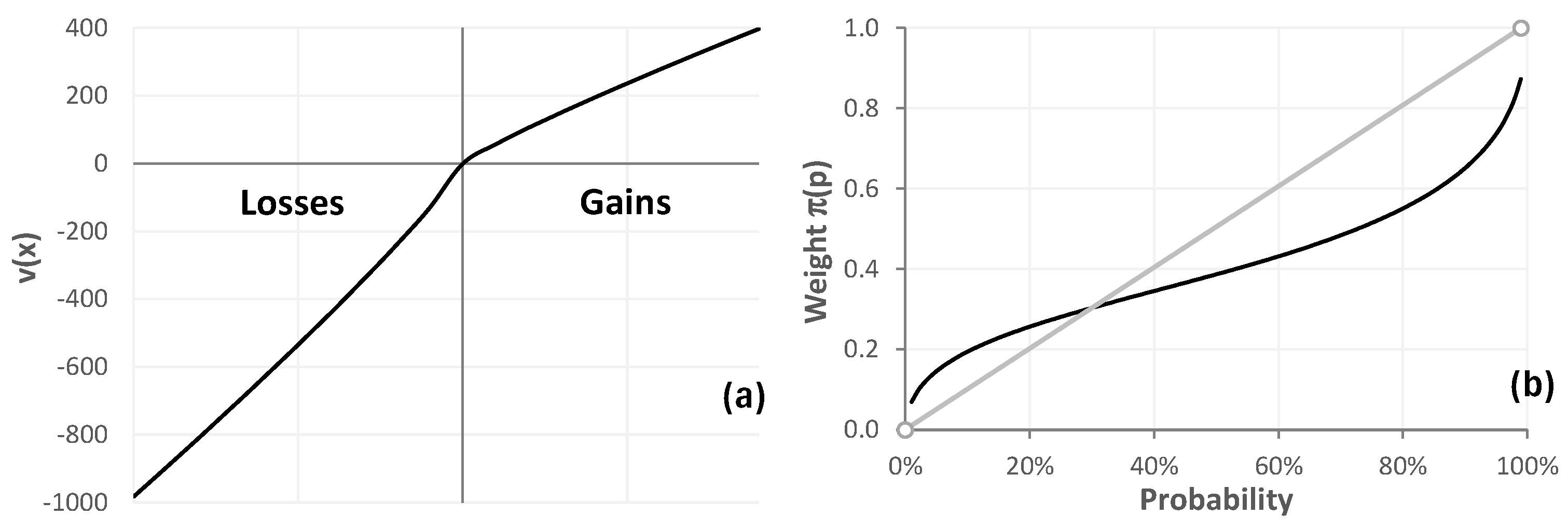
Economists traditionally model decision-making using utility functions, with expected utility theory assuming agents rationally maximize probability-weighted outcomes (von Neumann & Morgenstern, 1944). In reality, however, decision-making systematically deviates from this rational benchmark. Prospect theory (PT; Kahneman & Tversky, 1979) has become the prevailing behavioral framework, modeling decisions relative to a reference point and capturing two key departures from rationality. First, individuals exhibit loss aversion, whereby losses are weighted more heavily than equivalent gains. Second, responses to changes in outcomes are nonlinear, diminishing as outcomes move further from the reference point. These properties are formalized in the value function given by:

$$\begin{gathered} v\left(x\right)=x^{\alpha } \mathrm{f}\mathrm{o}\mathrm{r} x\ge 0 \\ v\left(x\right)=-\lambda {\left(-x\right)}^{\beta } \mathrm{f}\mathrm{o}\mathrm{r} x<0, \\ \mathrm{w}\mathrm{h}\mathrm{e}\mathrm{r}\mathrm{e} \alpha ,\beta ,\lambda >0 \mathrm{a}\mathrm{n}\mathrm{d} \lambda >1 \mathrm{c}\mathrm{a}\mathrm{p}\mathrm{t}\mathrm{u}\mathrm{r}\mathrm{i}\mathrm{n}\mathrm{g} \mathrm{l}\mathrm{o}\mathrm{s}\mathrm{s} \mathrm{a}\mathrm{v}\mathrm{e}\mathrm{r}\mathrm{i}\mathrm{o}\mathrm{n} \end{gathered}$$

(1)

PT further incorporates probability weighting, whereby objective probabilities are transformed into subjective decision weights. This captures the empirical tendency to overweight low-probability events and underweight high-probability events (see Figure 1):

$$\pi \left(p\right)={\displaystyle \frac{p^{\gamma }}{{\left(p^{\gamma }+{\left(1-p\right)}^{\gamma }\right)}^{\frac{1}{\gamma }}}}$$

(2)

with $0\le \gamma \le 1$.

These features are central to modeling depositor behavior, as they influence how individuals perceive bank failure risk and potential losses. Incorporating PT allows the model to capture heterogeneous and nonlinear responses to risk, which are critical in the context of bank runs.

Beyond individual decision-making, withdrawal behavior spreads socially, propagating through depositor networks much like a virus—each withdrawal increasing perceived risk for others and triggering further withdrawals in a self-reinforcing cycle. Shiller (2019) formalizes this analogy, showing that economic narratives spread through social networks following epidemic-like dynamics. Cookson et al. (2025) provide empirical support, finding that negative sentiment tweets during the SVB collapse significantly amplified run dynamics, with social media serving as a contagion mechanism rather than merely reflecting existing fundamentals. Standard equilibrium models struggle to capture these emergent dynamics, assuming representative agents and aggregate behavior. Agent-based models, by contrast, are well suited to representing heterogeneous depositors, localized interactions, and the nonlinear feedback loops through which individual decisions escalate into systemic runs.

2.3. Agent-Based Modeling Approaches

Santos and Nakane (2021) extend the DD framework within an ABM setting, showing how payout thresholds influence the incidence of bank runs and market concentration. While their results highlight the importance of depositor characteristics in shaping system dynamics, the model retains stylized assumptions and does not incorporate deposit insurance. Chan-Lau (2017) develops ABBA, an ABM of the banking system that models bank balance sheet dynamics and depositor withdrawals across a heterogeneous banking sector. Although the framework captures a wide range of bank-level decision processes, depositor behavior is governed by exogenous withdrawal probabilities, and neither deposit insurance nor behavioral decision-making under uncertainty is incorporated.

The broader ABM literature has focused predominantly on interbank contagion and systemic risk, with bank run dynamics and deposit insurance remaining comparatively underexplored. This paper addresses that gap by presenting a novel modeling framework that integrates heterogeneous depositors, prospect theory-based decision functions, and explicit fear propagation within a single ABM to quantify the impact of deposit insurance coverage on bank run risk.

3. Materials and Methods

Our ABM of bank runs is influenced by the foundational work of Diamond and Dybvig (1983) on bank run modeling. Building upon this framework, our model incorporates several enhancements, including a mechanism for fear propagation, PT utility, and probability functions to capture depositor behavior. We also expand the functionality of bank balance sheet management and introduce a structural default model based on Merton’s (1974) model to assess each bank’s likelihood of failure, which informs depositor decisions. The model is implemented in R (version 2025.09.2) with computationally intensive functions written in C++ and integrated via the Rcpp package (Eddelbuettel & François, 2011).

3.1. Banks’ Behavior

Banks operate under a standard maturity transformation structure, funding assets through deposits ($D$) and short-term debt ($S{T}_{debt}$). Assets consist of short-term liquid assets ($S{T}_{assets}$) and longer-term loans ($L{T}_{assets}$), earning returns x% and y%, respectively, while liabilities incur interest at rates i% (deposits) and r% (short-term debt). The balance sheet identity holds:

$$Equity=Assets-Liabilities$$

Credit losses on long-term assets follow a Bernoulli process with daily probability f, with loss severity equal to g% of total assets.

Table 1. Banks’ balance sheet (Source: Author).

Assets	Liabilities
$S{T}_{assets}$: Short-term assets (cash) at $x\%$ interest	$S{T}_{debt}$ Short-term debt at $r$% interest
$L{T}_{assets}$: Long-term assets (loans) $y\%$ interest, incur daily credit losses, $c$ Frequency following $Ber\left(f\right)$ with severity $g\%$	D: Deposits at $i$% interest
	Equity: Equity (balancing item)

summarizes the balance sheet structure.

At the initial time ($t=0$), banks commence with an initial solvency status ($So{l}_0$). Solvency is the quotient of total assets and total liabilities:

$$Sol={\displaystyle \frac{S{T}_{assets}+L{T}_{assets}}{S{T}_{debt}+D}}$$

(3)

A bank is deemed insolvent if $Sol<1$, at which point it exits the simulation. Banks manage liquidity through a rule-based asset-liability management (ALM) framework. The reserve ratio and net reserve ratio are defined as:

$$rr={\displaystyle \frac{S{T}_{assets}}{D}}$$

(4)

$$ne{t}_{rr}={\displaystyle \frac{S{T}_{assets}-S{T}_{debt}}{D}}$$

(5)

The ALM rule set maintains these ratios within predefined bounds. Surplus liquidity is allocated to long-term assets, while deficits are financed through short-term debt or, if constraints bind, through the liquidation of long-term assets at a discount.

The bank’s balance sheet dynamics determine its probability of default (PD), which is used by depositors in their withdrawal decisions. Following Merton (1974), PD is computed as:

$$P\left(A_{t+s}<L_{t+s}\right)\approx P\left(A_{t+s}<L_t\right)=\mathsf{\Phi }\left(-{\mathrm{d}}_2\right)$$

(6)

where

• $d_2=d_1-{\sigma }_A\sqrt{s}$
• $d_1={\displaystyle \frac{\ln \left(\frac{A_t}{L_t}\right)+s({\mu }_A+0.5{\sigma }_A^2)}{{\sigma }_A\sqrt{s}}}$
• $s=$ time horizon in time steps (days)
• $t=\mathrm{t}\mathrm{h}\mathrm{e} \mathrm{c}\mathrm{u}\mathrm{r}\mathrm{r}\mathrm{e}\mathrm{n}\mathrm{t} \mathrm{t}\mathrm{i}\mathrm{m}\mathrm{e} \mathrm{s}\mathrm{t}\mathrm{e}\mathrm{p}$
• $A_t=S{T}_{asset{s}_t}+L{T}_{asset{s}_t}$
• $L_t=D_t+S{T}_{deb{t}_t}$
• ${\mu }_A=\mathrm{r}\mathrm{o}\mathrm{l}\mathrm{l}\mathrm{i}\mathrm{n}\mathrm{g} \mathrm{d}\mathrm{a}\mathrm{i}\mathrm{l}\mathrm{y} \mathrm{g}\mathrm{r}\mathrm{o}\mathrm{w}\mathrm{t}\mathrm{h} \mathrm{r}\mathrm{a}\mathrm{t}\mathrm{e} \mathrm{o}\mathrm{f} A_t \mathrm{o}\mathrm{b}\mathrm{s}\mathrm{e}\mathrm{r}\mathrm{v}\mathrm{e}\mathrm{d} \mathrm{o}\mathrm{v}\mathrm{e}\mathrm{r} \mathrm{p}\mathrm{r}\mathrm{e}\mathrm{v}\mathrm{i}\mathrm{o}\mathrm{u}\mathrm{s} 30 \mathrm{t}\mathrm{i}\mathrm{m}\mathrm{e} \mathrm{s}\mathrm{t}\mathrm{e}\mathrm{p}\mathrm{s}$
• ${\sigma }_A=\mathrm{r}\mathrm{o}\mathrm{l}\mathrm{l}\mathrm{i}\mathrm{n}\mathrm{g} \mathrm{d}\mathrm{a}\mathrm{i}\mathrm{l}\mathrm{y} \mathrm{v}\mathrm{o}\mathrm{l}\mathrm{a}\mathrm{t}\mathrm{i}\mathrm{l}\mathrm{i}\mathrm{t}\mathrm{y} \mathrm{o}\mathrm{f} A_t \mathrm{o}\mathrm{b}\mathrm{s}\mathrm{e}\mathrm{r}\mathrm{v}\mathrm{e}\mathrm{d} \mathrm{o}\mathrm{v}\mathrm{e}\mathrm{r} \mathrm{t}\mathrm{h}\mathrm{e} \mathrm{p}\mathrm{r}\mathrm{e}\mathrm{v}\mathrm{i}\mathrm{o}\mathrm{u}\mathrm{s} 30 \mathrm{t}\mathrm{i}\mathrm{m}\mathrm{e} \mathrm{s}\mathrm{t}\mathrm{e}\mathrm{p}\mathrm{s}$.

The model evaluates PD over a 30-day horizon, reflecting the short-term risk horizon relevant for depositor decision-making.

3.2. Depositor Behavior

Each depositor is endowed with initial wealth ($w_0$), which may be uniform or drawn from a distribution (e.g., Pareto) and allocates this endowment to a single bank. Interest accrues daily. At each time step, depositors decide whether to withdraw based on one of three mechanisms: (i) random withdrawal, (ii) risk-based withdrawal, or (iii) fear-based withdrawal. Upon withdrawal, the depositor reallocates their full balance to a randomly selected solvent bank.

3.2.1. Random Withdrawal

At the beginning of each time step, a fixed percentage, $r_{withdraw}$, of total depositors are randomly selected to initiate withdrawals, mirroring the occurrence of spontaneous, non-financially motivated withdrawals in bank deposits. This form of withdrawal serves to approximate a baseline level of random withdrawal, independent of the financial health of the bank.

3.2.2. Risk-Based Withdrawal

Risk-based withdrawal is modeled for a subset of depositors who respond to bank-specific risk. We distinguish between informed and uninformed depositors, where only a proportion ℎ of depositors condition their decisions on the bank’s probability of default (PD), consistent with evidence that only a subset of depositors actively respond to risk signals (Gorton, 1988; Iyer & Puri, 2012).

Informed depositors evaluate the expected utility of maintaining their deposits using PT. Withdrawal occurs when the perceived value of remaining invested falls below zero. Unlike conventional approaches that apply PT to absolute changes in wealth, we apply the value function to percentage changes, allowing for heterogeneity in initial wealth levels and ensuring outcomes are evaluated relative to individual reference points.

Bank-specific PDs are obtained from the Merton model (Section 3.1). These probabilities are transformed using the Prelec (1998) weighting function, capturing empirically observed probability distortions, including the overweighting of small probabilities and underweighting of large probabilities (Kahneman & Tversky, 1979; Tversky & Kahneman, 1992). The weighting functions for gains and losses are given by:

$$\begin{gathered} w^{+}\left(p\right)=\exp \left(-{\left(-\mathit{ln}\left(p\right)\right)}^{\gamma }\right) \mathrm{f}\mathrm{o}\mathrm{r} \mathrm{g}\mathrm{a}\mathrm{i}\mathrm{n}\mathrm{s} \mathrm{a}\mathrm{n}\mathrm{d} \\ {w}^{-}\left(p\right)=\exp \left(-{\left(-\mathit{ln}\left(p\right)\right)}^{\delta }\right) \mathrm{f}\mathrm{o}\mathrm{r} \mathrm{l}\mathrm{o}\mathrm{s}\mathrm{s}\mathrm{e}\mathrm{s} \end{gathered}$$

(7)

where $\gamma <\delta ; \gamma ,\delta \in \left(0;1\right] \gamma <\delta ; \gamma ,\delta \in \left(0;1\right]$.

In (7), the Prelec probability weighting functions for gains and losses were quoted separately to capture the observed phenomenon, as demonstrated by Tversky and Kahneman (1992), wherein individuals tend to exhibit a more pronounced overweighting of small probabilities and underweighting of high probabilities when confronted with gains compared to losses ($\gamma <\delta$).

Depositors utilize these adjusted probabilities to assess the significance of potential gains and losses, with their combined impact influencing the decision to withdraw funds (8). Our analysis assumes only deposit amounts exceeding the deposit insurance threshold, denoted $d_{treshold}$, are subject to risk.

$$\mathrm{if}\left\{\begin{array}{c} v\left({∆}_{gain}\right)w^{+}\left(p\right)+v\left({∆}_{loss}\right)w^{-}\left(p\right)\ge 0;\hspace{1em}\mathrm{then} \mathrm{keep} \mathrm{deposit} \mathrm{invested}\\ v\left({∆}_{gain}\right)w^{+}\left(p\right)+v\left({∆}_{loss}\right)w^{-}\left(p\right)<0; \hspace{1em}\mathrm{then} \mathrm{withdraw} \mathrm{deposit}\end{array}\right.$$

(8)

where:

• ${∆}_{gain}={\displaystyle \frac{w_t{\left(1+i\%\right)}^{30}-w_t}{w_t}}={\left(1+i\%\right)}^{30}\{i\%=\mathrm{d}\mathrm{a}\mathrm{i}\mathrm{l}\mathrm{y} \mathrm{d}\mathrm{e}\mathrm{p}\mathrm{o}\mathrm{s}\mathrm{i}\mathrm{t} \mathrm{i}\mathrm{n}\mathrm{t}\mathrm{e}\mathrm{r}\mathrm{e}\mathrm{s}\mathrm{t} \mathrm{r}\mathrm{a}\mathrm{t}\mathrm{e}\}$
• ${∆}_{loss}={\displaystyle \frac{\mathrm{m}\mathrm{i}\mathrm{n}(d_{threshold}-w_t; 0)}{w_t}}$
• $w_t=\mathrm{s}\mathrm{t}\mathrm{a}\mathrm{r}\mathrm{t}\mathrm{i}\mathrm{n}\mathrm{g} \mathrm{w}\mathrm{e}\mathrm{a}\mathrm{l}\mathrm{t}\mathrm{h} \mathrm{a}\mathrm{t} t+1$
• $w_t=w_{t-1}\left(1+i\%\right) \mathrm{f}\mathrm{o}\mathrm{r} t\ge 1$
• $v\left(x\right) \mathrm{a}\mathrm{s} \mathrm{s}\mathrm{p}\mathrm{e}\mathrm{c}\mathrm{i}\mathrm{f}\mathrm{i}\mathrm{e}\mathrm{d} \mathrm{i}\mathrm{n} \left(1\right)$
• $w^{+}\left(p\right) \mathrm{a}\mathrm{n}\mathrm{d} w^{-}\left(p\right) \mathrm{a}\mathrm{s} \mathrm{s}\mathrm{p}\mathrm{e}\mathrm{c}\mathrm{i}\mathrm{f}\mathrm{i}\mathrm{e}\mathrm{d} \mathrm{i}\mathrm{n} \left(7\right)$
• $p \mathrm{a}\mathrm{s} \mathrm{d}\mathrm{e}\mathrm{f}\mathrm{i}\mathrm{n}\mathrm{e}\mathrm{d} \mathrm{i}\mathrm{n} \left(6\right)$
• $\mathrm{N}\mathrm{o}\mathrm{t}\mathrm{e}, \mathrm{i}\mathrm{f} d_{threshold}=0 \mathrm{t}\mathrm{h}\mathrm{e}\mathrm{n} {∆}_{loss}=-1$ for all depositors.

This formulation captures heterogeneous risk perceptions, probability distortions, and nonlinear valuation of gains and losses. Given the binary outcome structure of the model (gain versus loss), the use of standard PT yields results equivalent to cumulative PT (CPT) and is therefore sufficient for the present setting.

3.2.3. Fear-Based Withdrawal

The third withdrawal mechanism captures herding behavior in bank runs. Depositors form beliefs through random interactions with other depositors at the same bank. At each time step, every depositor observes the actions of n randomly selected peers, with interactions independently resampled across periods.

For each observed depositor who has withdrawn, the observing depositor withdraws with probability ℓ ∈ [0, 1]. Specifically, for each such observation, a draw u ∼ U(0, 1) is made, and withdrawal occurs if u < ℓ. This process is applied sequentially across observed withdrawals within the period.

This formulation implies that withdrawal behavior is increasing in exposure to withdrawing peers, generating stochastic contagion. Unlike deterministic threshold models, the probabilistic structure allows heterogeneous responses under identical conditions. The parameter ℓ governs sensitivity to observed withdrawals, while n determines the rate at which information propagates through the system.

Following withdrawal, depositors move to another bank, where the process repeats. Aggregate dynamics therefore emerge endogenously from local interactions, giving rise to potential cascade effects.

This approach is consistent with the literature on coordination and contagion in financial markets, including Keynes’s (1936) “beauty contest” analogy and subsequent work on expectation-driven behavior. While the model abstracts from factors such as media effects and institutional trust, it provides a tractable representation of fear-driven withdrawal dynamics.

3.3. Model Specification and Parameterization

3.3.1. Model Setup

The ABM is initialized at t = 0 by constructing a population of m depositors and q banks, with all state variables fully parameterized ex ante. Depositors are assigned to banks via uniform random allocation and characterized by initial wealth, behavioral parameters governing herding (encounter frequency and fear threshold), and decision-theoretic parameters derived from PT (risk preferences, loss aversion, and probability weighting). A subset of depositors is designated as informed, capable of forward-looking risk-based withdrawal decisions over a fixed horizon. Banks are initialized with stylized balance sheets determined by an initial solvency ratio, decomposing assets into liquid and illiquid components and liabilities into deposits and (initially zero) short-term debt. Liquidity management is governed by a reserve ratio corridor (minimum, target, maximum), while profitability and funding costs are driven by exogenous interest rates on assets and liabilities. Credit risk is introduced via stochastic losses on long-term assets, modeled as Bernoulli arrivals with fixed severity, providing the fundamental source of solvency deterioration.

Table 2. Depositor parameter estimates.

Parameter Symbol (Description)	Assigned Value/Distribution
$m$ (total depositors)	100,000
$n$ (number of friends)	5
$l\%$ (fear threshold)	30%
$h\%$ (informed depositors)	10%
$w_0$ (starting wealth)	Equal distribution
$\alpha$ (sensitivity to gains)
$\beta$ (sensitivity to losses)
$\lambda$ (loss aversion)
$\gamma$ (probability distortion for gains)
$\delta$ (probability distortion for losses)
$s$ (time horizon)	30
$r_{withdraw}$ (random withdraw)	2% p.a.

and

Table 3. Bank parameter estimates.

Parameter Symbol (Description)	Assigned Value/Distribution
$q$ (total banks)	20
$S_0$ (initial solvency)	1.05
$r_{max}$ (maximum reserve ratio)	15%
$r{r}_{target}$ (target reserve ratio)	12.5%
$r{r}_{min}$ (minimum reserve ratio)	10%
$x$ (interest earned on short-term assets)	2%
$r$ (interest paid on short-term debt)	2%
$i$ (interest paid to depositors)	1%
$y$ (interest earned on long-term assets)	4%
$h$ (haircut on forced sale of long-term assets)	40%
$f$ (frequency of credit losses on long-term assets)	$Ber\left({\displaystyle \frac{1}{90}}\right)$
$g$ (severity of credit losses on long-term assets)	[0.5%; 4%]

present parameterization.

3.3.2. Model Run

From t = 1 to T, the system evolves through a repeated sequence of depositor and bank interactions that jointly determine systemic stability. At each time step, withdrawals arise through three channels: exogenous random switching, endogenous risk-based decisions by informed depositors using a PT valuation of expected gains, losses, and default risk, and contagion-driven fear withdrawals triggered by observed peer behavior. Banks then pay interest, update balance sheets via asset–liability management rules (borrowing, asset reallocation, or fire sales subject to reserve constraints), and absorb stochastic credit losses, with solvency and default probabilities recalculated dynamically. Banks failing solvency or depositor viability constraints exit the system, and their depositors are reallocated to surviving institutions, propagating stress. The process iterates until either a terminal time horizon is reached or the system collapses to a single surviving bank, allowing the emergence of bank run dynamics and systemic outcomes to be endogenously characterized.

3.3.3. Depositor Parameter Estimates

Parameterizing an ABM to reflect real-world behavior is inherently challenging due to limited data and behavioral complexity. We therefore adopt empirically grounded estimates where available and rely on economically reasonable assumptions otherwise, with the objective of capturing the key mechanisms driving bank run dynamics under varying levels of deposit insurance.

The simulation includes 100,000 depositors, balancing realism and computational tractability. Herding behavior is modeled via daily peer interactions: each depositor observes five others within the same bank, with a 30% independent probability of withdrawing upon observing a withdrawal, generating increasing cumulative withdrawal likelihoods. A baseline random withdrawal rate of 2% per annum captures normal liquidity needs. All depositors begin with equal wealth in the base case, though alternative distributions (e.g., Pareto) are considered in extensions.

A proportion of 10% of depositors is assumed to be informed and capable of risk-based withdrawals. This assumption is broadly consistent with evidence that only a minority of depositors actively responds to bank risk (Iyer & Puri, 2012). Decision-making under risk is modeled using PT: preference parameters for gains and losses are drawn from β distributions, while loss aversion follows a Γ distribution, parameterized to cross-country evidence (Rieger et al., 2016). Probability weighting follows the Prelec (1998) specification, with parameters based on Booij et al. (2009) and constrained such that loss-side distortion exceeds gain-side distortion, consistent with Tversky and Kahneman (1992).

Depositor decisions are formed over a 30-day horizon, reflecting a short-term focus on bank stability. Volatility in behavioral parameters is introduced to capture population heterogeneity. Table 2 summarizes the full depositor parameterization.

3.3.4. Bank Parameter Estimates

We parameterize the banking sector to reflect stylized features of the U.S. system, balancing empirical realism with tractability. The model comprises 20 banks, each initially serving 5000 depositors. Banks are initialized with a solvency ratio of 1.05 (equity-to-assets ≈ 4.8%), consistent with observed leverage and above Basel III requirements. Liquidity management is governed by a reserve corridor, with a minimum of 10%, a target of 12.5%, and a maximum of 15%, aligned with historical Federal Reserve requirements (Federal Reserve, 2024).

Interest rates are set to ensure a realistic and positive intermediation spread: deposits earn 1%, while short-term borrowing and lending occur at 2%, and long-term assets yield 4%. In stress scenarios, forced asset sales incur a 40% haircut, consistent with Basel Framework collateral haircut requirements for physical and real estate collateral (BIS, 2023). Credit risk is introduced via Bernoulli shocks to long-term assets, with daily probability f and fixed severity g%, parameterized to generate plausible failure dynamics.

Our simulations continue until either a single bank remains or the simulation reaches its maximum duration, which is set at three years, corresponding to 1095-time steps. Table 3 summarizes the full bank parameterization.

4. Results

The outcomes under the base case configuration are discussed in this section, followed by a series of alternative scenarios, where we compare the results to the base case to draw key insights and assess the robustness of the model’s outcomes.

4.1. Base Run Results

Table A1. Simulated bank survival rates.

Credit Loss	Deposit Insurance
	0%	25%	50%	60%	70%	80%	90%	95%	97.5%	100%
0.50%	100%	100%	100%	100%	100%	100%	100%	100%	100%	100%
0.75%	100%	100%	100%	99%	100%	100%	100%	100%	100%	100%
0.90%	93%	96%	96%	97%	98%	98%	98%	99%	99%	100%
1.00%	61%	76%	91%	84%	91%	92%	95%	96%	97%	100%
1.10%	57%	41%	77%	78%	75%	86%	90%	92%	93%	100%
1.15%	19%	31%	48%	53%	59%	74%	84%	91%	92%	100%
1.20%	10%	21%	21%	35%	61%	75%	83%	86%	89%	100%
1.25%	7%	7%	28%	41%	30%	48%	63%	78%	85%	100%
1.30%	0%	11%	16%	10%	10%	52%	59%	72%	81%	100%
1.40%	2%	0%	0%	6%	4%	11%	40%	58%	73%	100%
1.50%	0%	0%	0%	0%	0%	1%	12%	31%	53%	98%
1.75%	0%	0%	0%	0%	0%	0%	0%	8%	15%	89%
2.00%	0%	0%	0%	0%	0%	0%	0%	0%	3%	71%
2.50%	0%	0%	0%	0%	0%	0%	0%	0%	0%	23%
3.00%	0%	0%	0%	0%	0%	0%	0%	0%	0%	2%
3.50%	0%	0%	0%	0%	0%	0%	0%	0%	0%	0%
4.00%	0%	0%	0%	0%	0%	0%	0%	0%	0%	0%

and

Table A2. Simulated bank survival days.

Credit Loss	Deposit Insurance
	0%	25%	50%	60%	70%	80%	90%	95%	97.5%	100%
0.50%	1095	1095	1095	1095	1095	1095	1095	1095	1095	1095
0.75%	1090	1090	1090	1086	1090	1095	1095	1095	1095	1095
0.90%	1029	1057	1061	1066	1074	1077	1075	1088	1087	1095
1.00%	825	896	1009	967	1013	1027	1055	1064	1071	1095
1.10%	777	674	921	919	898	975	1012	1026	1040	1095
1.15%	512	594	708	766	795	897	968	1021	1030	1095
1.20%	414	511	546	642	785	897	956	987	1008	1095
1.25%	389	398	571	682	629	727	833	938	979	1094
1.30%	300	427	522	510	524	765	816	900	955	1095
1.40%	286	316	382	399	454	541	710	822	900	1094
1.50%	236	262	298	313	334	387	589	681	807	1087
1.75%	198	215	254	269	290	291	378	516	582	1035
2.00%	176	204	220	233	244	257	328	372	477	970
2.50%	124	147	166	189	197	196	247	286	320	711
3.00%	131	136	142	153	159	186	191	216	269	431
3.50%	118	117	127	135	145	141	180	188	208	318
4.00%	102	108	120	113	119	132	142	165	183	253

report simulated bank survival rates and average bank survival days, respectively, across credit loss severities (0.5–4.0%) and deposit insurance coverage levels (0–100%). Each cell reflects the average outcome from 20 simulations, so the tables are based on a total of 3400 simulations.

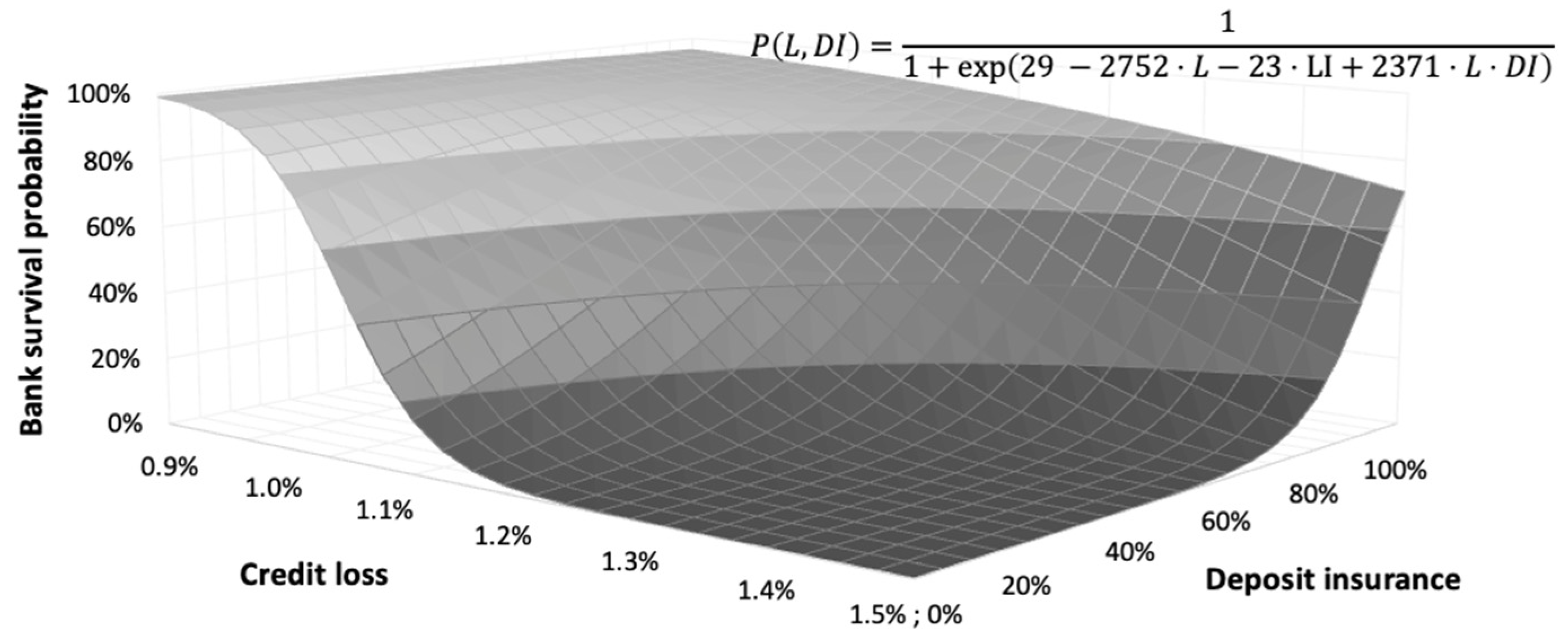
Figure 2 presents the estimated two-dimensional logistic surface fitted to the simulated survival probabilities, with Figure 3 showing the corresponding contour representation. For clarity, Figure 2 focuses on the interval 0.9–1.5% credit losses, which contains the inflection region of the surface. Below 0.9%, failure is negligible across deposit insurance levels, whereas above 1.5%, failure becomes widespread regardless of coverage. The economically relevant variation therefore occurs within this intermediate range, where deposit insurance shifts the failure threshold.

Figure 2 presents the estimated two-dimensional logistic surface mapping credit loss severity, $L$ and deposit insurance coverage, $DI$, into bank survival probability:

$$P(L,DI)={\displaystyle \frac{1}{1+\mathrm{e}\mathrm{x}\mathrm{p}\left[-({\beta }_0+{\beta }_{1}L+{\beta }_{2}DI+{\beta }_{3}LDI)\right]}}$$

The fitted surface explains 95% of the variation in the simulated survival rates (response-scale variance-explained $R^2=0.95$), indicating that the joint nonlinearity of the simulation outcomes is well captured by the parametric representation.

The surface exhibits pronounced threshold dynamics. The 50% survival boundary, defined by $P(L,DI)=0.5$, is characterized by

$${\beta }_0+{\beta }_{1}L+{\beta }_{2}DI+{\beta }_{3}LDI=0,$$

which yields the critical loss threshold

$$L^{*}(DI)={\displaystyle \frac{-{\beta }_0-{\beta }_{2}DI}{{\beta }_1+{\beta }_{3}DI}}$$

Evaluated at the estimated coefficients, the implied tipping point shifts materially with coverage. Under zero deposit insurance, the critical loss level is $L^{*}\left(0\right)=1.06\%$. At 50% coverage, the threshold increases to 1.14% and under full coverage to 1.73%. Thus, deposit insurance shifts the collapse boundary rightward in loss space but does not eliminate it.

The interaction term (${\beta }_3>0$) implies that the effect of deposit insurance depends on stress severity. In the absence of stress, coverage has a negligible impact on failure risk. As losses approach the transition region, however, deposit insurance materially alters the system’s stability boundary. Once losses exceed the upper transition region, the surface flattens as survival probability approaches zero and additional coverage produces diminishing marginal effects.

The geometry of the surface therefore characterizes the model’s stability landscape: a narrow transition band separates a stable regime from systemic collapse, and policy operates primarily by shifting the location of this boundary rather than altering the structure of the transition itself. Figure 3 decomposes the three-dimensional surface into conditional cross-sections to clarify the underlying mechanics.

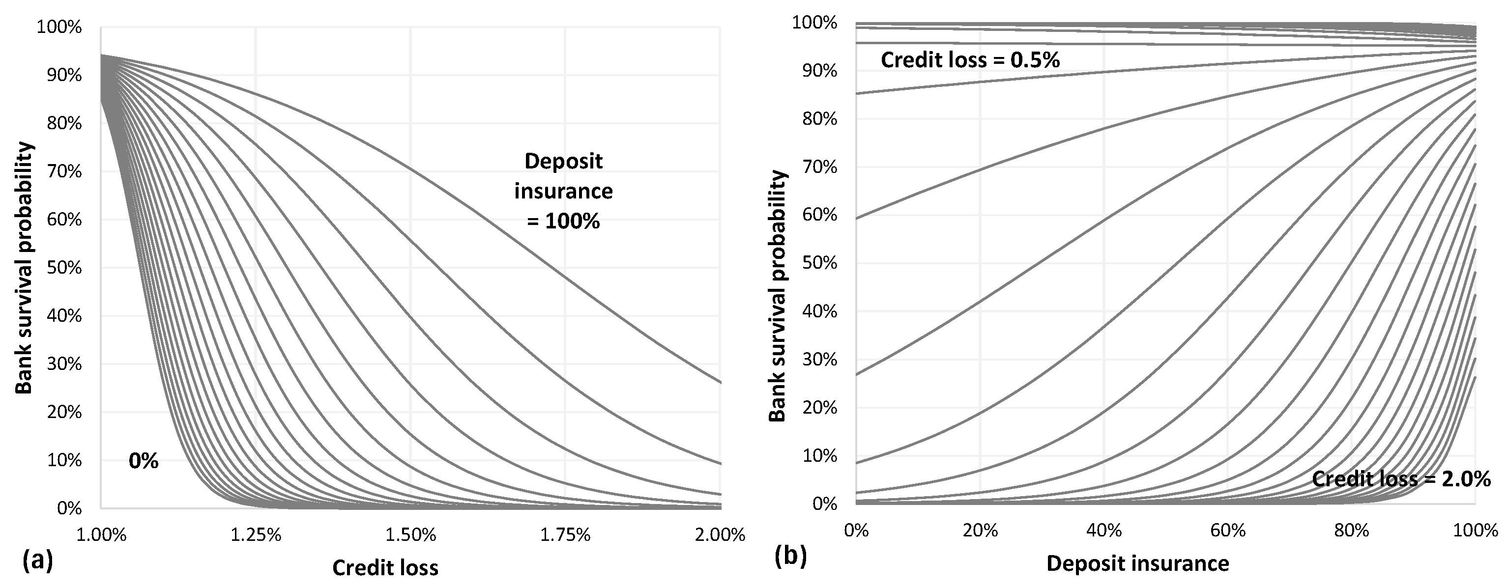
Panel (a) plots survival probability as a function of credit loss for fixed levels of deposit insurance. The curves exhibit the characteristic “S-shaped” profile implied by the logistic structure. The steep gradient between 1.0% and 1.3% losses reflects the endogenous amplification mechanisms embedded in the simulation model. Outside this interval, the curves flatten: for losses below 1%, survival probabilities approach unity; for losses above 2%, survival approaches zero regardless of coverage.

Panel (b) presents the complementary perspective: survival probability as a function of deposit insurance for fixed stress levels. The marginal effect of deposit insurance is

$${\displaystyle \frac{\partial P}{\partial DI}}=P(1-P)({\beta }_2+{\beta }_{3}L),$$

which highlights two key features.

First, policy effectiveness is state-dependent. The term $P(1-P)$ peaks in the transition region, implying that coverage changes matter most when the system operates near its critical boundary. When the system is already stable ($P\approx 0$) or already collapsing ($P\approx 1$), additional insurance has a limited influence.

Second, the interaction coefficient implies that the stabilizing impact of deposit insurance increases with stress severity within the transition band. In log-odds terms, a 10% increase in coverage increases survival odds by a factor of $\mathrm{e}\mathrm{x}\mathrm{p}\left(0.10\right({\beta }_2+{\beta }_{3}L\left)\right)$. At moderate stress levels (e.g., $L=1.5\%$), a 10 percentage-point increase in coverage increases survival odds by 263%. At lower stress levels (e.g., $L=1\%$), the corresponding increase is 11%, reflecting the state-dependent nature of the policy effect.

Together, the cross-sections confirm that deposit insurance primarily operates by shifting the tipping threshold rather than flattening the slope of the transition. The model therefore implies a regime-dependent policy effect: insurance meaningfully extends systemic resilience near the critical stress region but cannot prevent collapse under sufficiently severe losses.

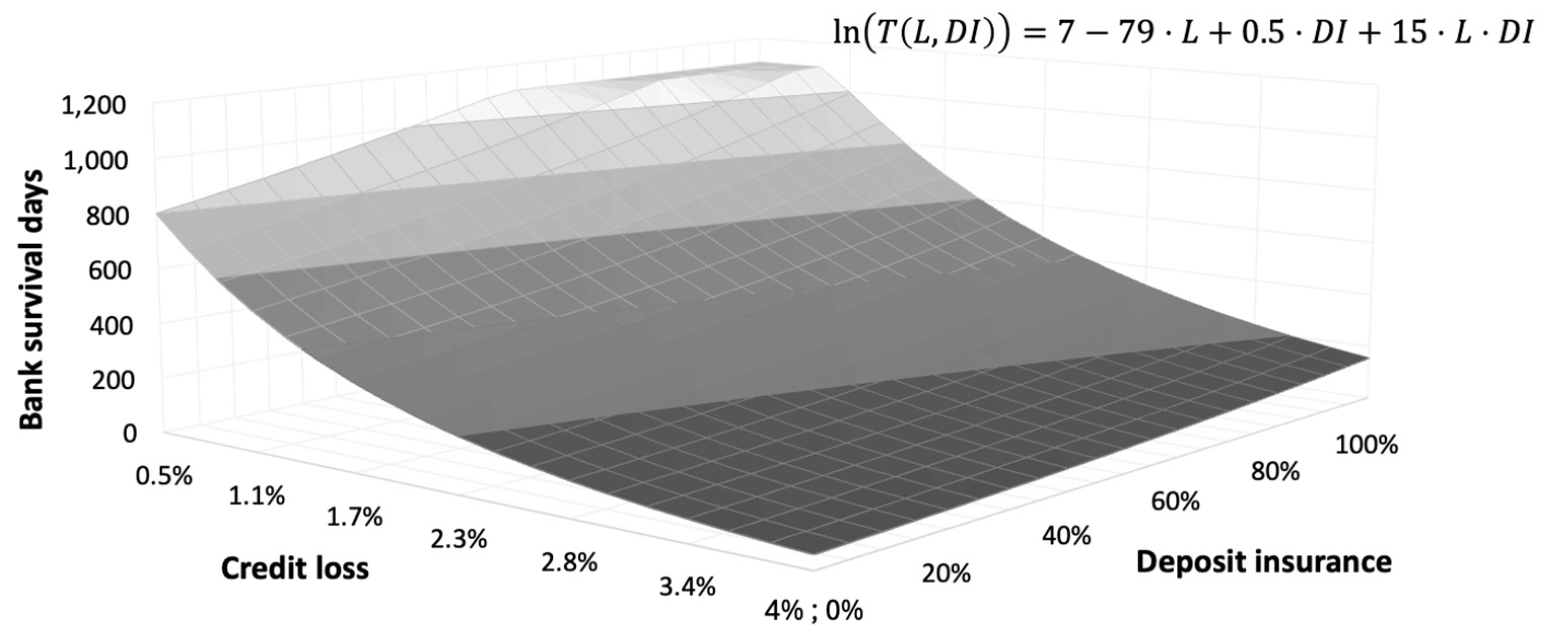
Figure 4 presents the estimated log-linear survival time surface, with Figure 5 showing the associated contours. The surface quantifies the incremental survival time attributable to deposit insurance under a range of credit losses.

The fitted model takes the form

$$\mathrm{l}\mathrm{o}\mathrm{g} T(L,DI)={\alpha }_0+{\alpha }_{1}L+{\alpha }_{2}DI+{\alpha }_3(L·DI),$$

with predictions reported on the original time scale via $\widehat{T}(L,DI)=\exp \left(\log \widehat{T}(L,DI)\right)$. The log-linear specification provides a close approximation to the simulated survival outcomes ($R^2=0.86$ on the log scale), offering a parsimonious representation of how policy and stress jointly shape time-to-failure.

The surface implies a strongly nonlinear mapping from the state variables to survival time. Holding coverage fixed, survival declines steeply as credit losses increase, consistent with a multiplicative (approximately exponential) deterioration in resilience under more severe stress. Holding credit losses fixed, predicted survival increases with deposit insurance and does so at an accelerating rate as coverage approaches full insurance, reflecting the model’s amplification of confidence effects when the safety net becomes sufficiently salient.

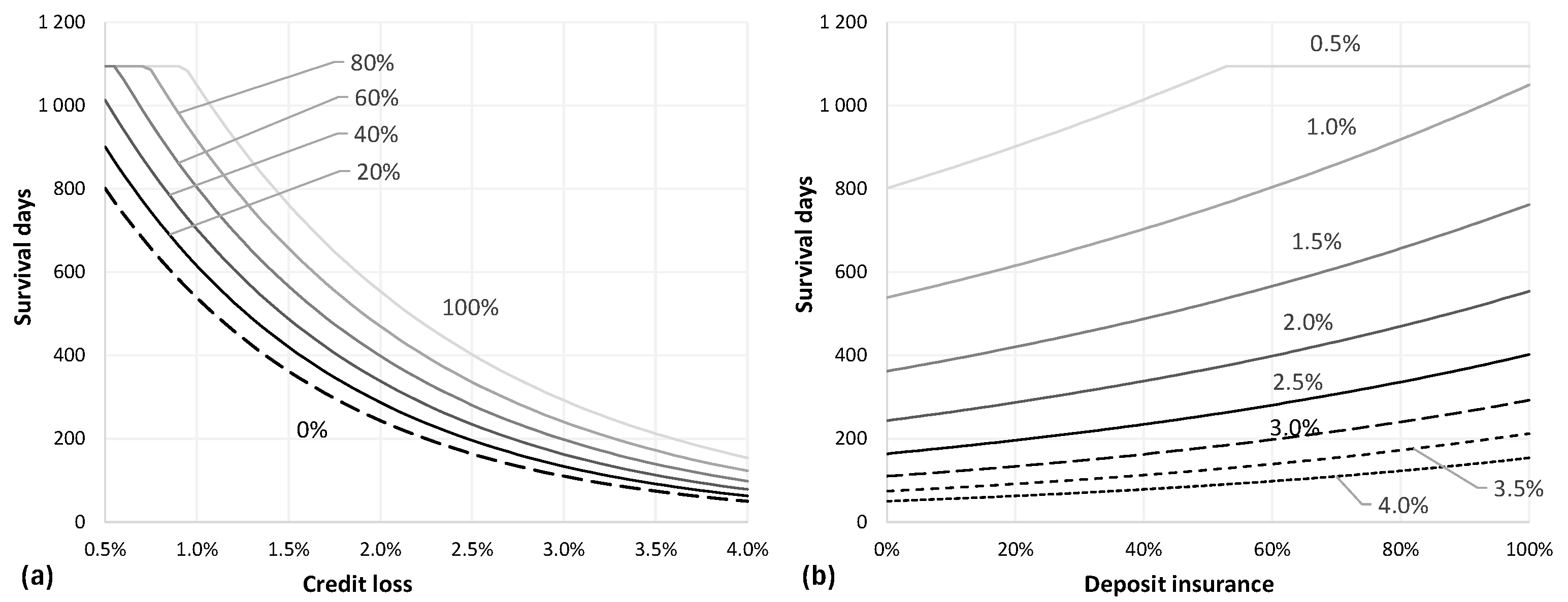
The interaction term (${\alpha }_3>0$) indicates state dependence: the marginal effect of deposit insurance is weaker at low stress and becomes more pronounced under higher losses. In other words, deposit insurance primarily matters in the region where failure is imminent under the zero-insurance benchmark and where time-to-failure remains responsive to stabilization policies. This pattern is consistent with the notion that the safety net is most consequential when the system operates close to the boundary between solvency and collapse. Figure 5 provides cross-sections of the fitted survival surface to isolate the comparative statics in each dimension.

Panel (a) plots survival days as a function of credit loss severity for fixed deposit insurance levels. The curves display approximately exponential decay in L, consistent with the log-linear structure: equal increments in losses reduce survival multiplicatively rather than additively. Higher coverage shifts the entire schedule upward, indicating that deposit insurance increases not only the level of survival but also the range of stress severities over which banks remain active for a non-trivial duration.

Panel (b) plots survival days as a function of deposit insurance for fixed stress levels. The convex shape of the curves reflects the exponential back-transformation of the log-linear model: linear improvements in $Log T$ translate into accelerating gains in tons on the day scale. The spacing across loss curves shows that insurance benefits are strongly state dependent: for moderate stresses, the increase in survival from higher coverage is substantial, whereas under extreme stresses, survival remains limited even at high insurance levels. This pattern underscores a key implication of the model: deposit insurance shifts the distribution of time-to-failure meaningfully in the transition region but exhibits diminishing returns once shocks are sufficiently severe that failure is effectively unavoidable within the simulation horizon.

Figure 4 and Figure 5 quantify deposit insurance as a resilience-shifting policy: it extends time-to-failure most in the region where the system is vulnerable but not yet in near-immediate collapse, while its incremental benefit becomes small in both low-stress states (where survival is long regardless of policy) and very high-stress states (where failure is rapid regardless of coverage).

4.2. Scenario 1: Wealth Distributions

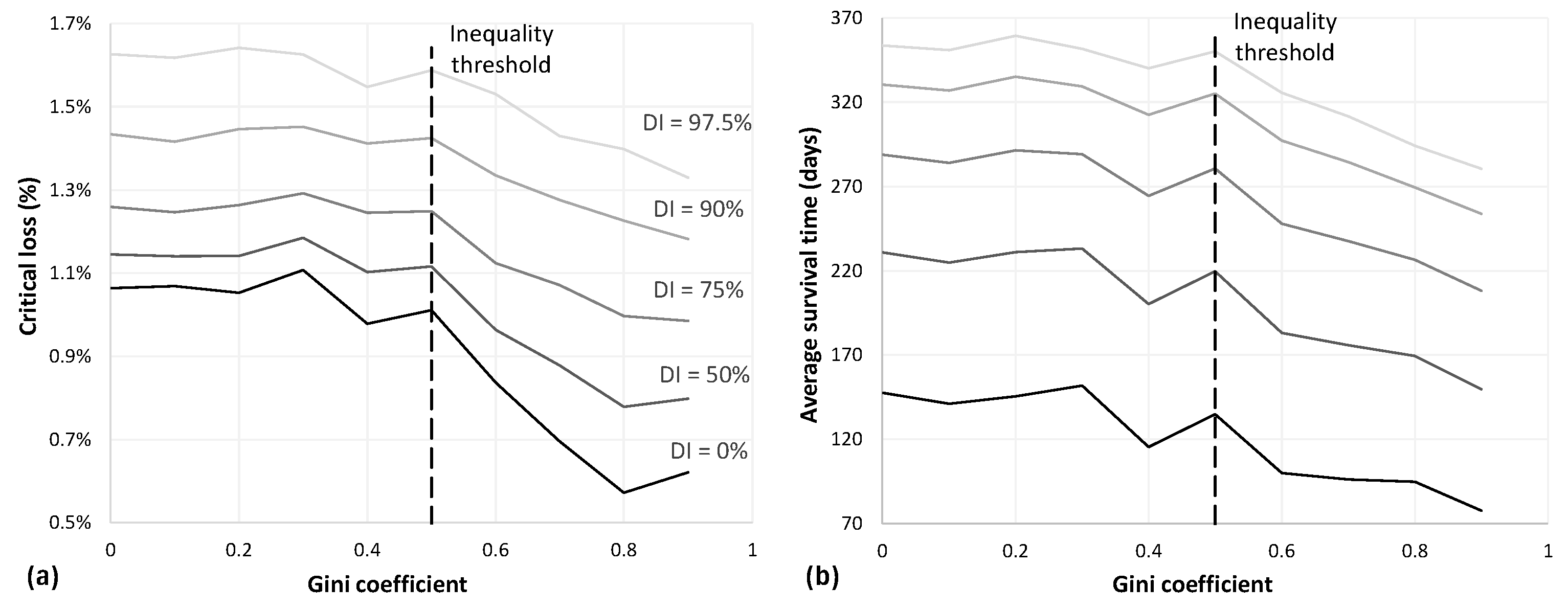
This section examines the impact of wealth inequality, as measured by the Gini coefficient, on systemic stability. The full set of estimated survival probability and survival time surfaces for each wealth distribution is available from the author upon request. Figure 6 collapses these surfaces into two policy-relevant statistics: (a) the critical loss threshold and (b) average survival time under severe stress, computed over credit losses ranging from 1.5% to 4.0%.

Figure 6a plots the critical loss threshold as a function of the Gini coefficient for different levels of deposit insurance. The critical loss is defined as the level of credit losses at which the probability of system survival equals 50% and therefore represents the boundary between stability and systemic collapse. Two key patterns emerge.

4.2.1. Critical Loss Threshold

First, wealth inequality systematically erodes resilience. The critical loss threshold remains relatively stable at low inequality levels but declines sharply beyond a Gini coefficient of approximately 0.5, indicating that extreme wealth concentration introduces a nonlinear destabilizing effect.

Second, deposit insurance shifts the stability boundary upward but does not alter its shape. Higher coverage increases the stress the system can absorb before failure, but the downward slope persists across all insurance levels—deposit insurance improves resilience but does not offset the destabilizing effects of extreme wealth concentration.

4.2.2. Survival Time Under Severe Stress

Figure 6b presents average survival time under severe stress (credit losses between 1.5% and 4.0%) as a function of the Gini coefficient. This loss range is used because bank failure rates approach 100% throughout, ensuring survival durations are not affected by censoring. Wealth inequality reduces survival time in a systematic and nonlinear manner, with the same threshold observed as in panel (a)—the effect becomes materially stronger beyond a Gini coefficient of 0.5. Deposit insurance shifts the survival-time curves upward across all inequality levels, extending the number of days banks remain active under stress, but does not alter the fundamental relationship between inequality and collapse dynamics.

Wealth inequality therefore primarily affects the location of the stability boundary rather than its underlying structure, with a consistent threshold effect emerging at a Gini coefficient of approximately 0.5 across both resilience and survival time dimensions.

4.3. Scenario 2: Depositor Risk Aversion

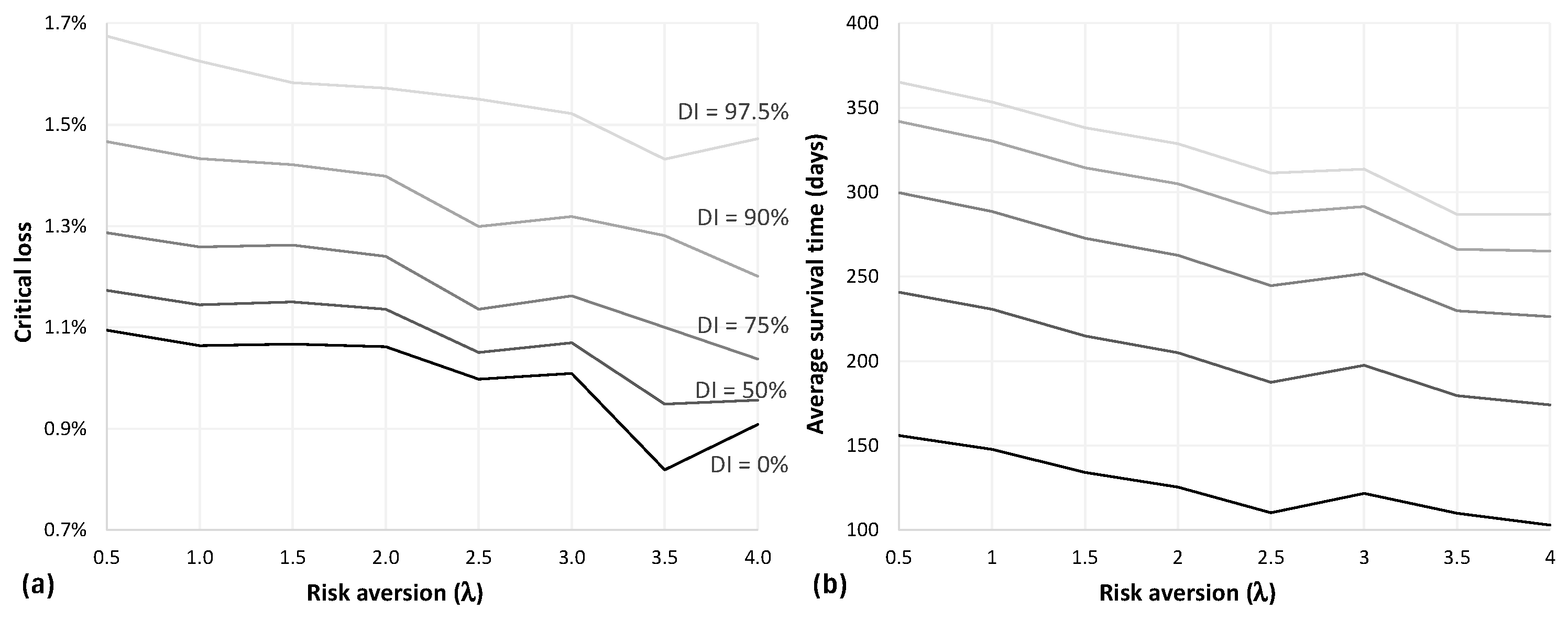
This section examines how depositor risk aversion, parameterized by λ, affects systemic stability. Figure 7 summarizes the underlying survival probability and survival time surfaces into two policy-relevant metrics: (a) the critical loss threshold and (b) average survival time under severe stress.

Figure 7a plots the critical loss threshold as a function of depositor risk aversion for different levels of deposit insurance. Values of λ = 0.5, 1, 1.5, 2, 2.5, 3, 3.5 and 4 correspond to average depositor PD thresholds of 3.8%, 2.7%, 2.1%, 1.7%, 1.5%, 1.3%, 1.1% and 1.0%, respectively, when deposit insurance is set at 50%. That is, these thresholds represent the average probability of bank failure over the next 30 days at which depositors choose to withdraw their funds.

4.3.1. Critical Loss Threshold

Deposit insurance shifts the critical loss threshold upward across all levels of risk aversion, increasing the magnitude of shocks the system can absorb before collapse. Consistent with the base results, this confirms that deposit insurance operates as a level-shifting mechanism for resilience.

However, it does not materially alter the shape of the relationship between risk aversion and the critical loss. Across most coverage levels, the threshold declines approximately linearly as λ increases, indicating that deposit insurance does not change the underlying mechanism through which depositor risk sensitivity drives fragility, but rather raises the collapse boundary.

The deterioration is most pronounced in the absence of deposit insurance. At 0% coverage, increases in risk aversion lead to a sharp decline in the critical loss threshold, with the system becoming highly fragile at elevated levels of λ. While higher coverage mitigates this effect by shifting the stability boundary upward, the persistent downward slope shows that increased risk aversion continues to erode resilience even under substantial insurance.

4.3.2. Survival Time Under Severe Stress

Figure 7b presents the average survival time under severe stress (credit losses between 1.5% and 4.0%) as a function of depositor risk aversion. Unlike the wealth distribution scenario, average survival time initially declines approximately linearly as λ increases from 0.5 to 2.5, after which the rate of decline flattens between λ = 2.5 and 4. This pattern is consistent across all levels of deposit insurance. The result is intuitive, as the average PD threshold declines more rapidly over the lower range of λ, while the reduction becomes more gradual at higher levels. As before, higher deposit insurance increases overall survival time, shifting the curves upward without altering their shape, indicating that deposit insurance affects the level of resilience but not the underlying dynamics of collapse.

Depositor risk aversion therefore erodes resilience continuously but does not alter the fundamental mechanism through which deposit insurance operates.

4.4. Scenario 3: Depositor Awareness

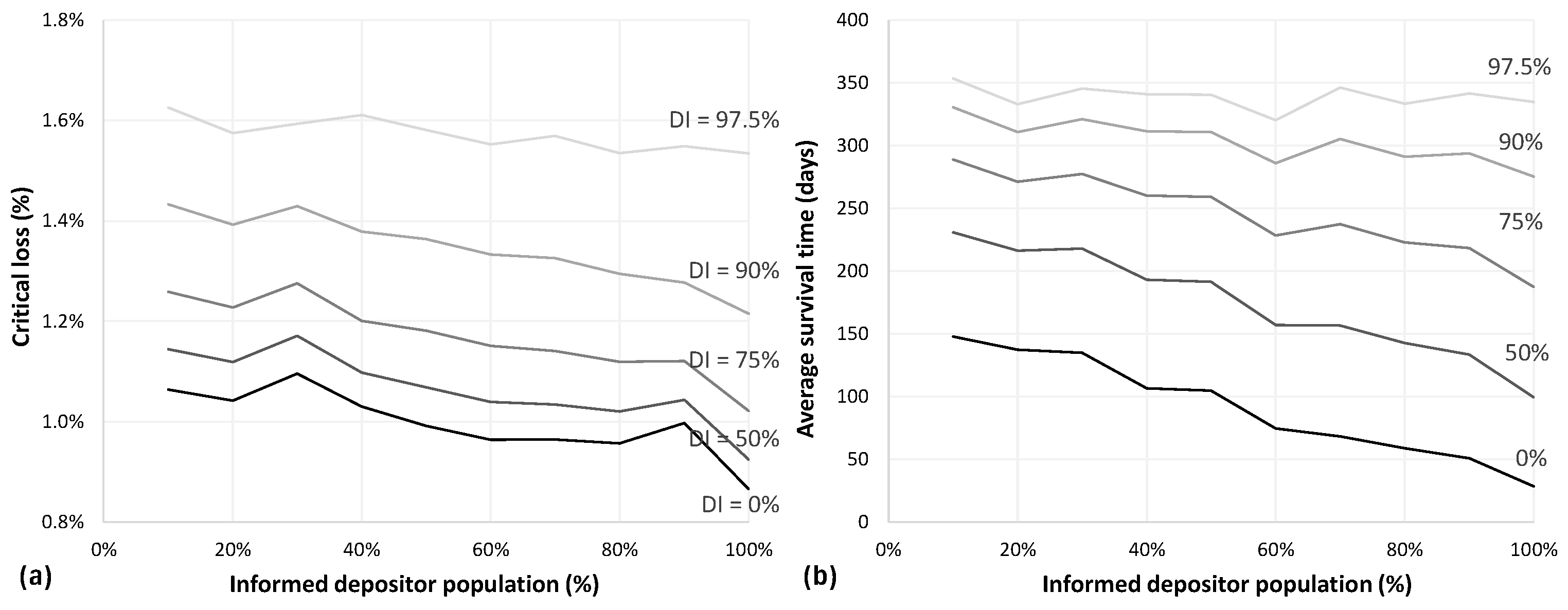
This section examines how depositor awareness, defined as the proportion of depositors informed about bank risk, affects systemic stability. Figure 8 summarizes the underlying survival probability and survival time surfaces into two policy-relevant metrics: (a) the critical loss threshold and (b) average survival time under severe stress.

4.4.1. Critical Loss Threshold

Figure 8a plots the critical loss threshold as a function of depositor awareness for different levels of deposit insurance. From 10% to 30% of the population being informed, the critical loss remains relatively stable. Beyond this point, from 30% to 100%, a strong and approximately linear decline emerges across all levels of deposit insurance. The shape of this relationship is consistent across coverage levels, indicating that deposit insurance shifts the level of resilience without altering the underlying dynamics. System vulnerability is highest when all depositors are informed, suggesting that once the share of informed (or sophisticated) depositors exceeds 30%, the stability of the banking system materially deteriorates.

The relationship between awareness and stability is gradual but persistent, with 30% informed depositors acting as a soft tipping point—similar to the Gini coefficient of 0.5 identified in the wealth inequality scenario, but without the same abruptness. Beyond this point, the steady decline in the critical loss reflects the role of information as a coordination mechanism: as more depositors observe and respond to risk signals, the likelihood of self-reinforcing withdrawal dynamics increases materially.

4.4.2. Survival Time Under Severe Stress

Figure 8b presents average survival time under severe stress (credit losses between 1.5% and 4.0%) as a function of depositor awareness. Survival time exhibits a clear and approximately linear decline as the share of informed depositors increases. Unlike the wealth and risk aversion scenarios, deposit insurance here not only shifts survival time upward but also dampens the sensitivity of collapse dynamics to awareness. At 0% deposit insurance, survival time falls sharply from 150 to 50 days as the informed population increases from 10% to 100%, whereas at 90% coverage the decline is more moderate, from roughly 330 to 260 days. This suggests that while depositor awareness consistently accelerates collapse, higher deposit insurance mitigates the magnitude of this effect.

In summary, depositor awareness persistently erodes systemic resilience beyond the 30% tipping point, with deposit insurance shifting the stability boundary upward without altering its slope in the critical loss dimension, but actively dampening the sensitivity of collapse dynamics to information diffusion in the survival time dimension.

4.5. Scenario 4: Depositor ‘Fear Thresholds’

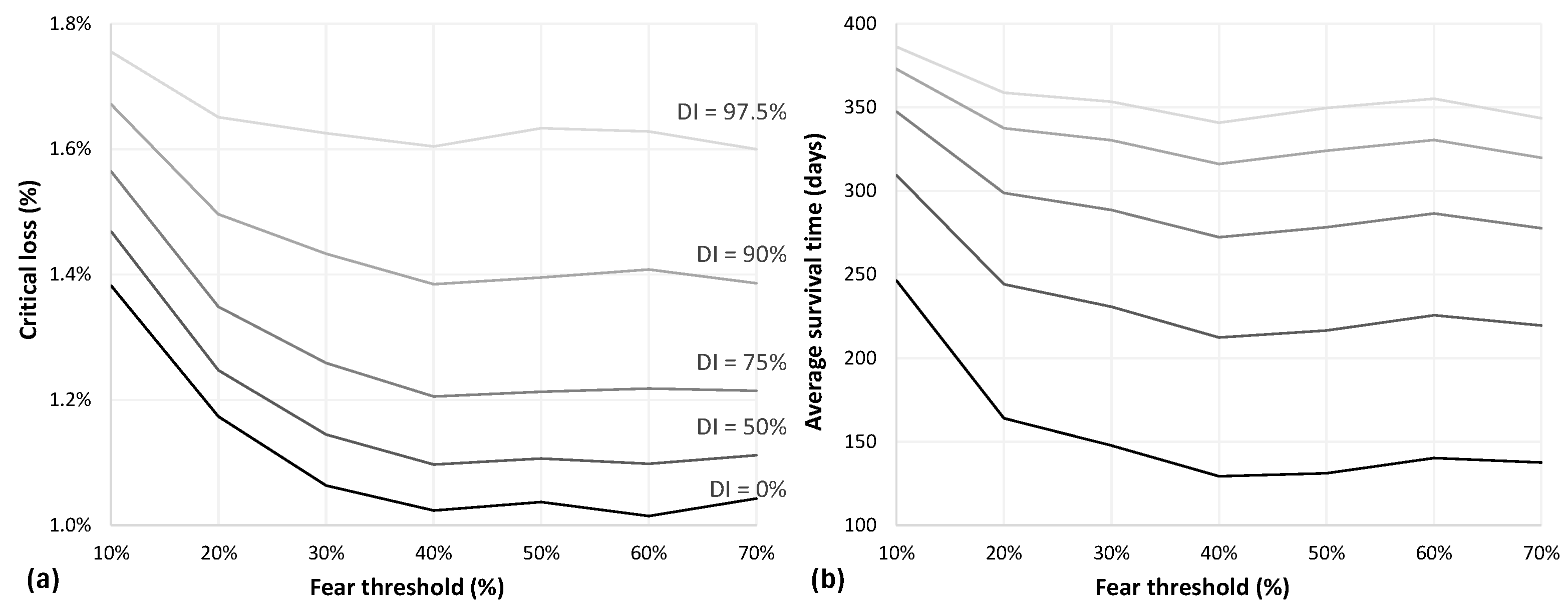
This section examines how depositor fear thresholds, the proportion of observed withdrawals required to trigger a withdrawal decision, affect systemic stability. Figure 9 summarizes the underlying survival probability and survival time surfaces into two policy-relevant metrics: (a) the critical loss threshold and (b) average survival time under severe stress.

Figure 9a plots the critical loss threshold as a function of depositor fear thresholds for different levels of deposit insurance. As the contagion parameter increases from 10% to 40%, the critical loss declines markedly, albeit at a diminishing rate. Beyond this range, from 40% to 70%, the relationship flattens, indicating that the system has reached a region of near-maximal vulnerability. This pattern suggests that systemic fragility is highly sensitive to the strength of peer influence at low to moderate levels of contagion, where small increases substantially amplify coordinated withdrawal behavior.

4.5.1. Critical Loss Threshold

At higher levels of contagion, further increases have a limited marginal impact, as withdrawal dynamics are already strongly synchronized—once peer effects strengthen sufficiently, the system behaves as if it is close to full coordination. Greater susceptibility to peer influence therefore materially reduces the system’s shock tolerance, reinforcing behavioral contagion as a key driver of systemic risk.

4.5.2. Survival Time Under Severe Stress

Figure 9b presents average survival time under severe stress (credit losses between 1.5% and 4.0%) as a function of depositor fear thresholds. As in Figure 9a, survival time declines most sharply at lower to moderate levels of contagion, after which the rate of decline flattens as withdrawal behavior becomes sufficiently synchronized and additional increases in contagion have limited marginal impact on collapse dynamics.

In summary, fear thresholds primarily destabilize the system through early coordination effects, with deposit insurance consistently shifting resilience upward but unable to alter the fundamental relationship between peer influence and systemic fragility.

5. Discussion

Diamond and Dybvig (1983) describe bank runs as a coordination problem, proposing deposit insurance as the solution. Our results confirm that deposit insurance is effective—shifting both the critical loss threshold and time-to-failure upward—but does not fully resolve the coordination problem. Even under full coverage, prospect theory-based decision making and herding behavior ensure that coordination dynamics persist, confirming that deposit insurance is not a panacea and cannot substitute for strong bank fundamentals. This is consistent with Amador and Bianchi (2024), who show that policy responses are fundamentally limited when crises are coordination-driven.

Depositor concentration materially undermines stability, with a Gini coefficient exceeding 0.5 producing significantly worse outcomes—directly echoing SVB, where a concentrated base of uninsured corporate depositors created acute coordination vulnerability (Metrick, 2024; Rose, 2023; Cipriani et al., 2024). Regulators should incorporate depositor concentration into supervisory frameworks alongside capital and liquidity metrics, building on but extending beyond what the Net Stable Funding Ratio under Basel III currently captures (BIS, 2013).

Risk aversion continuously erodes resilience but lacks a sharp tipping point. Depositor awareness exhibits a soft tipping point at 30%, beyond which informed depositors act as coordination amplifiers (Cookson et al., 2025; Kiss et al., 2012). Near-complete deposit insurance coverage can substantially mitigate this effect, suggesting that high coverage levels partially neutralize the destabilizing influence of a sophisticated depositor minority.

Fear propagation follows epidemic-like dynamics (Shiller, 2019), compounding the awareness effect as fear transmission accelerates once a critical mass of informed depositors responds to risk signals. Early and credible communication of financial strength is therefore a more effective stabilization tool than attempting to restore confidence once withdrawal dynamics are synchronized.

Taken together, these findings demonstrate the value of ABMs in revealing that systemic fragility is not a binary outcome but a continuous function of behavioral and distributional parameters with identifiable tipping points. Policymakers should treat deposit insurance as one instrument within a broader stability framework that also addresses concentration risk, information dynamics, and behavioral contagion.

6. Conclusions

This paper presents a novel ABM framework that simultaneously incorporates heterogeneous depositors, prospect theory-based decision making, and explicit deposit insurance coverage testing—an integration absent from existing banking ABMs. The results confirm that deposit insurance raises the critical loss threshold and extends time-to-failure, but does not eliminate underlying coordination dynamics—irrational decision making and herding ensure withdrawal behavior persists even under full coverage. Strong bank fundamentals remain the most reliable safeguard against systemic collapse.

The scenarios further reveal that depositor concentration, awareness, and fear propagation interact with deposit insurance in ways that materially shape outcomes. A Gini coefficient exceeding 0.5 represents a tipping point beyond which fragility accelerates significantly. Critically, depositor awareness and fear propagation prove potent destabilizers regardless of underlying fundamentals—once a critical mass of depositors monitors bank health or fear begins to spread, withdrawal dynamics accelerate rapidly. Trust and perception are therefore as consequential as balance sheet strength, and maintaining depositor confidence is as important a policy objective as ensuring adequate capital and liquidity.

This paper demonstrates the value of ABMs in identifying behavioral tipping points and quantifying the conditional effectiveness of regulatory instruments. Future extensions incorporating interbank dynamics, macroeconomic variables, and cross-jurisdictional institutional differences would further enrich the framework’s policy relevance.

7. Limitations

While this paper advances the ABM literature by explicitly modeling depositor behavior and deposit insurance—dimensions that existing banking ABMs have largely overlooked in favor of interbank contagion—several limitations warrant acknowledgment.

First, the model excludes direct interbank transactions such as interbank lending, repos, and derivative exposures, with contagion operating solely through depositor behavior. Incorporating interbank liquidity contagion and counterparty risk represents a natural and valuable extension.

Second, the model operates at the micro-behavioral level and does not incorporate macroeconomic variables such as interest rate shocks, inflation, or monetary tightening—factors that played a significant role in the 2023 US banking crisis. Future work integrating macro-financial dynamics would substantially enrich the framework.

Third, deposit insurance is the sole regulatory instrument modeled. Lender of last resort facilities, emergency liquidity support, and government guarantee schemes are absent, and future extensions incorporating these instruments would allow for richer policy scenario analysis.

Fourth, model parameters are based on empirically grounded estimates rather than calibration to granular bank-level data. Future work using institution-specific data would improve empirical precision and allow for comparisons across bank types and sizes.

Finally, depositors are treated as a homogeneous behavioral population. Segmenting depositors into retail, corporate, and high-net-worth categories and testing across different jurisdictions and deposit insurance regimes would extend the framework’s generalizability and policy relevance.

References

1. Amador, M., & Bianchi, J. (2024). Bank runs, fragility, and credit easing. The American Economic Review, 114(7), 2073–2110. [Google Scholar] [CrossRef]
2. BIS. (2013). Basel III: The liquidity coverage ratio and liquidity risk monitoring tools. Bank for International Settlements. Available online: https://www.bis.org/publ/bcbs238.pdf (accessed on 12 January 2026).
3. BIS. (2023). Basel framework: Credit risk—Internal ratings-based approach, CRE32.11. Bank for International Settlements. Available online: https://www.bis.org/basel_framework/chapter/CRE/32.htm (accessed on 9 February 2026).
4. Booij, A. S., van Praag, B. M. S., & van de Kuilen, G. (2009). A parametric analysis of prospect theory’s functionals for the general population. Theory and Decision, 68(1–2), 115–148. [Google Scholar] [CrossRef]
5. Calomiris, C. W., & Jaremski, M. (2016). Deposit insurance: Theories and facts. National Bureau of Economic Research. [Google Scholar] [CrossRef]
6. Chan-Lau, J. A. (2017). ABBA: An agent-based model of the banking system. International Monetary Fund. [Google Scholar]
7. Cipriani, M., Eisenbach, T., & Kovner, A. (2024). Tracing bank runs in real time. Federal Reserve Bank of Richmond Working Papers, 24(10), 1–46. [Google Scholar] [CrossRef]
8. Cookson, J. A., Fox, C., Gil-Bazo, J., Imbet, J. F., & Schiller, C. (2025). Social media as a bank run catalyst. Journal of Financial Economics, 176, 104218. [Google Scholar] [CrossRef]
9. De Roux, N., & Limodio, N. (2023). Deposit insurance and depositor behavior: Evidence from Colombia. The Review of Financial Studies, 36(7), 2721–2755. [Google Scholar] [CrossRef]
10. Diamond, D. W., & Dybvig, P. H. (1983). Bank runs, deposit insurance and liquidity. Journal of Political Economy, 91(3), 401–419. [Google Scholar] [CrossRef]
11. Eddelbuettel, D., & François, R. (2011). Rcpp: Seamless R and C++ integration. Journal of Statistical Software, 40(8). [Google Scholar] [CrossRef]
12. Federal Reserve. (2024). Federal reserve board—Reserve requirements. Board of Governors of the Federal Reserve. Available online: https://www.federalreserve.gov/monetarypolicy/reservereq.htm (accessed on 17 December 2025).
13. Gertler, M., & Kiyotaki, N. (2015). Banking, liquidity, and bank runs in an infinite horizon economy. American Economic Review, 105(7), 2011–2043. [Google Scholar] [CrossRef]
14. Gorton, G. (1988). Banking panics and business cycles. Oxford Economic Papers, 40(4), 751–781. [Google Scholar] [CrossRef]
15. Iyer, R., & Puri, M. (2012). Understanding bank runs: The importance of depositor-bank relationships and networks. The American Economic Review, 102(4), 1414–1445. [Google Scholar] [CrossRef]
16. Kahneman, D., & Tversky, A. (1979). Prospect theory: An analysis of decision under risk. Econometrica, 47(2), 263–291. [Google Scholar] [CrossRef]
17. Kelly, M., & Gráda, C. Ó. (2000). Market contagion: Evidence from the panics of 1854 and 1857. American Economic Review, 90(5), 1110–1124. [Google Scholar] [CrossRef]
18. Keynes, J. M. (1936). The general theory of employment, interest and money. Macmillan. [Google Scholar]
19. Kiss, H. J., Rodriguez-Lara, I., & Rosa-García, A. (2012). On the effects of deposit insurance and observability on bank runs: An experimental study. Journal of Money, Credit and Banking, 44(8), 1651–1665. [Google Scholar] [CrossRef]
20. Merton, R. C. (1974). On the pricing of corporate debt: The risk structure of interest rates. The Journal of Finance, 29(2), 449. [Google Scholar] [CrossRef]
21. Metrick, A. (2024). The failure of silicon valley bank and the panic of 2023. Journal of Economic Perspectives, 38(1), 133–152. [Google Scholar] [CrossRef]
22. Prelec, D. (1998). The probability weighting function. Econometrica, 66(3), 497. [Google Scholar] [CrossRef]
23. Rieger, M. O., Wang, M., & Hens, T. (2016). Estimating cumulative prospect theory parameters from an international survey. Theory and Decision, 82(4), 567–596. [Google Scholar] [CrossRef]
24. Rose, J. (2023). Understanding the speed and size of bank runs in historical comparison. [online] research.stlouisfed.org. Available online: https://research.stlouisfed.org/publications/economic-synopses/2023/05/26/understanding-the-speed-and-size-of-bank-runs-in-historical-comparison (accessed on 11 November 2025).
25. Santos, T. R. E. d., & Nakane, M. I. (2021). Dynamic bank runs: An agent-based approach. Journal of Economic Interaction and Coordination, 16(3), 675–703. [Google Scholar] [CrossRef]
26. Shiller, R. J. (2019). Narrative economics. Princeton University Press. [Google Scholar] [CrossRef]
27. Tversky, A., & Kahneman, D. (1992). Advances in prospect theory: Cumulative representation of uncertainty. Journal of Risk and Uncertainty, 5(4), 297–323. [Google Scholar] [CrossRef]
28. von Neumann, J., & Morgenstern, O. (1944). Theory of games and economic behavior. Princeton University Press. [Google Scholar]
29. Weber, E. U., & Johnson, E. J. (2009). Decisions under uncertainty. In Neuroeconomics: Decision making and the brain (pp. 127–144). Academic Press. [Google Scholar] [CrossRef]
Figure 1. PT’s (a) value function with v x = x 0.88 for gains and v x = 2.25 x 0.88 for losses and (b) decision weight function π ( p ) with γ = 0.55 . Source: Weber and Johnson (2009).
Jrfm 19 00404 g001
Figure 2. Base run bank survival probability.
Jrfm 19 00404 g002
Figure 3. (a) Bank survival probability per credit loss level and (b) per deposit insurance level.
Jrfm 19 00404 g003
Figure 4. Base run bank survival days.
Jrfm 19 00404 g004
Figure 5. (a) Bank survival days per credit loss level and (b) per deposit insurance level.
Jrfm 19 00404 g005
Figure 6. (a) Critical loss threshold vs. wealth inequality and (b) average survival time under severe stress vs. wealth inequality.
Jrfm 19 00404 g006
Figure 7. (a) Critical loss threshold vs. risk aversion and (b) average survival time under severe stress vs. risk aversion.
Jrfm 19 00404 g007
Figure 8. (a) Critical loss threshold vs. depositor awareness and (b) average survival time under severe stress vs. depositor awareness.
Jrfm 19 00404 g008
Figure 9. (a) Critical loss threshold and (b) average survival time under stress vs. fear thresholds.
Jrfm 19 00404 g009