Does Exchange Rate Volatility Matter for Banking-Sector Financial Stability? A Global Analysis

Abstract

Exchange rate volatility has intensified in recent decades, yet its systematic implications for banking-sector stability remain contested. This study investigates whether exchange rate volatility constitutes a meaningful source of financial fragility using a global panel of 103 countries over the period 2000–2021. Financial stability is proxied by the banking-sector Z-score, while exchange rate volatility is estimated using a EGARCH-based framework to capture time-varying uncertainty. To address cross-sectional dependence, heterogeneity, and endogeneity, the analysis employs Driscoll–Kraay fixed effects, two-step system GMM, and quantile regressions. The results reveal that exchange rate volatility exerts a statistically and economically significant negative effect on banking stability, reducing Z-scores across countries and income groups. The findings remain robust across alternative specifications and estimators. Bank-level fundamentals—capitalisation, liquidity, and credit—enhance stability, whereas higher non-performing loans and risk exposure amplify fragility. Macroeconomic conditions also matter, with stronger growth, institutional quality and external balances supporting resilience, while inflation, economic policy uncertainty and expansionary government spending weaken stability. By integrating time-varying volatility modelling with dynamic panel techniques in a large cross-country setting, this study provides new global evidence that exchange rate volatility is not merely a macroeconomic fluctuation but a structural source of banking-sector risk. The findings carry important implications for macroprudential policy, foreign-exchange management, and coordinated monetary–fiscal responses aimed at safeguarding financial stability in open economies.

1. Introduction

Exchange rate volatility has been a persistent feature of the international monetary system since the collapse of the Bretton Woods arrangement. With the move away from fixed exchange rate regimes, currency values in many economies have become more sensitive to market conditions and external shocks. Exchange rate volatility typically intensifies during periods of global stress, including the Global Financial Crisis, the COVID-19 pandemic, and the recent phase of monetary tightening across advanced economies (International Monetary Fund, 2022; BIS, 2023). These episodes have again brought exchange rate movements into focus, highlighting their role in shaping national financial outcomes through interactions with domestic financial systems.

The potential for exchange rate volatility to impact banking systems through risk and balance-sheet channels makes it relevant for financial stability. Currency fluctuations can alter the domestic value of foreign-currency positions, place pressure on asset quality, and complicate funding conditions. In banking systems with exposure to international capital flows or currency mismatches, these effects may translate into higher risk and weaker resilience. As a result, exchange rate volatility is increasingly recognised as one of several factors that may shape banking-sector stability, operating alongside more established macroeconomic and financial determinants (International Monetary Fund, 2023; Bartram et al., 2015; Oyadeyi et al., 2024). At the same time, whether these effects are systematic or large enough to matter across countries remains an open question.

Theoretical contributions have long pointed out that the consequences of exchange rate volatility are unlikely to be uniform across economies. In particular, Bacchetta and van Wincoop (2000) emphasise that differences in institutional arrangements, adjustment processes, and financial structures largely shape how countries respond to currency fluctuations. Empirical results reflect this uncertainty. In some studies, higher exchange rate volatility is associated with greater financial stress, whereas in others the relationship weakens once banking-sector features and wider macroeconomic conditions are taken into account (Bartram et al., 2015; Hasanov et al., 2024; International Monetary Fund, 2023; Oyadeyi et al., 2026). Overall, the existing evidence does not point to a single or definitive role for exchange rate volatility in driving financial instability.

Consequently, this paper examines whether exchange rate volatility presents a systematic and economically meaningful source of banking-sector financial instability across countries, with direct implications for macroprudential regulation and exchange rate policy in open economies. More recent work points to methodological issues as one reason for these mixed findings. Estimated effects often depend on how volatility is measured, how global spillovers are treated, and whether heterogeneity across countries is allowed for in the empirical design (Hasanov et al., 2024; Okot et al., 2022). Using Exponential Generalised Autoregressive Conditional Heteroskedasticity (EGARCH)-type models and panel methods improves measurement, but it does not fully resolve identification problems. In broad cross-country samples, exchange rate volatility remains difficult to isolate, largely because cross-sectional dependence, differences in financial development, and institutional variation continue to affect inference and comparability.

Against this background, the literature has gradually moved away from trade-based explanations toward financial and balance-sheet transmission mechanisms operating through the banking sector. Recent studies emphasise balance-sheet effects, credit conditions, and risk-taking behaviour as channels through which exchange rate movements may influence financial stability (Bruno & Shin, 2020; Du & Schreger, 2022). Empirical evidence suggests that higher exchange rate volatility is often associated with weaker asset quality and higher non-performing loans, although the strength of these relationships varies across countries and over time (International Monetary Fund, 2023). This variation suggests that a broad, cross-country perspective is needed to better understand how exchange rate volatility interacts with banking-sector stability.

This study examines the relationship between exchange rate volatility and financial stability using a global sample of 103 countries over the period 2000–2021. Financial stability is proxied by the banking-sector Z-score, while exchange rate volatility is obtained using a EGARCH-based approach. The empirical framework is informed by the financial accelerator theory, which emphasises the amplification of external shocks, including currency movements, through bank balance sheets. Bank-level indicators and macroeconomic variables are included to reflect differences in financial conditions and economic environments across countries.

Exchange rate volatility is often discussed in macroeconomic terms, but this study shows that currency fluctuations can also pose a financial stability concern for banking systems, with effects that differ across countries. In this respect, the paper makes five main contributions. First, it offers global evidence on the relationship between exchange rate volatility and banking-sector stability using a large and diverse country sample unlike previous studies (Laeven & Levine, 2009; Oyadeyi, 2024; Agénor et al., 2026). Second, it focuses explicitly on financial stability rather than trade flows or firm-level outcomes, aligning the analysis with macroprudential policy concerns, a departure from Agénor et al. (2026), which focuses on middle-income countries. Third, it combines volatility modelling with dynamic panel techniques such as GMM, Driscoll–Kraay estimators within a panel data framework, alongside quantile regression and Economic Testing frameworks (e.g., CIPS, CADF, etc.) that account for cross-sectional dependence, heterogeneity, and endogeneity.

In addition, by using the banking-sector Z-score and incorporating both bank-level and macroeconomic controls, this study provides systematic, internationally comparable evidence on whether exchange rate volatility constitutes a meaningful source of financial instability, thereby advancing the frontier of knowledge on the nexus between exchange rate volatility and cross-border corporate financial stability. Finally, the study also contributes to the frontier of knowledge by analysing the impacts of economic policy uncertainty and institutional quality on financial stability to establish whether, in the presence of exchange rate volatility, these variables have consequential effects on financial stability. The findings showed that incorporating exchange rate volatility, institutional quality and economic policy uncertainty issues into the financial accelerator theory, provides an important transmission of external shocks to financial stability, thereby making them important determinants of financial stability within the sample. Therefore, exchange rate volatility and economic policy uncertainty are pragmatic external shocks that affect the stability of financial systems, while quality institutions are essential to mitigate these shocks, in line with the postulations of the financial accelerator theory.

The rationale for undertaking this study is because of the increased exposure of financial firms to foreign-exchange risks due to globalisation, economic uncertainty, global trade, geopolitical risks, foreign-currency borrowing, and the interconnections among financial markets. The unique motivation for the study arises from the observation that increased currency volatility, driven by global financial cycles, geopolitics, external shocks, or monetary policy spillovers, has increased firm instability, especially as it relates to firm balance sheets, input costs, investment choices, and profits. Considering the importance of firm stability for a stable macroeconomic, microeconomic, and financial environment, as well as for supporting economic and financial resilience, exchange rate volatility may affect the stability and resilience of macroeconomic and financial systems, posing dangers that may exacerbate global systemic and nonsystemic shocks. As a result, a global analysis on the effects of exchange rate volatility on the financial system across these countries will provide insights on how currency fluctuations affect financial stability and their survival across varying institutional and financial contexts, thereby guiding corporate risk management strategies and the formulation of effective exchange rate, monetary, and macroprudential policies.

The remainder of the paper is organised as follows. Section 2 critically examines the theoretical and empirical literature on exchange rate volatility and corporate financial stability, emphasising the ongoing debate over whether volatility destabilises, conditionally affects, or has no systematic impact on financial stability. Section 3 outlines the data, variables, and econometric methodology. Section 4 presents and discusses the empirical findings, and Section 5 concludes with policy implications and directions for future research.

2. Empirical Literature Review on Exchange Rate Volatility and Banking-Sector Financial Stability

Exchange rate volatility refers to the degree of fluctuation of a country’s currency value over time, particularly unpredictable movements relative to another currency or a group of currencies. Under fixed exchange rate systems, governments mainly determined currency values. Following the collapse of the Bretton Woods system, the global monetary system shifted toward flexible exchange rates, exposing currencies to fluctuations driven by market forces (Bacchetta & van Wincoop, 2000). Exchange rates react to a variety of factors in these systems, including changes in global investor confidence, risk sentiment, policy divergences, capital movements, macroeconomic fundamentals, and cross-border capital flows (International Monetary Fund, 2022; BIS, 2023). These factors can occasionally lead to financial crises. Together, these forces lead to instability during periods of financial stress.

In empirical research, exchange rate volatility is typically measured using statistical approaches such as standard deviations of exchange rate returns or conditional variance models (Kanas, 2003), particularly EGARCH-type specifications, which capture time-varying volatility and clustering effects (Hasanov et al., 2024). These models capture patterns such as volatility clustering and reflect how financial markets behave, particularly how sudden currency movements can sharply change the value of foreign-currency assets and liabilities. Therefore, measuring and analysing unexpected exchange rate volatility is more important for financial stability and risk management, as it creates uncertainty for banks and borrowers.

Financial stability describes the capacity of the financial system to absorb shocks without interrupting its essential functions, such as financial intermediation and risk allocation (International Monetary Fund, 2023). In practice, stability is most often evaluated at the banking-sector level because banks play a central role in providing credit and liquidity. Financial stability depends on a banking system maintaining strong capital buffers, adequate liquidity, and controlled credit risk, even under challenging macroeconomic conditions (Demirgüç-Kunt & Detragiache, 2011).

In practice, the Z-score is one of the most widely used indicators for measuring financial stability. It measures a bank’s distance from insolvency by combining profitability, leverage, and earnings volatility (Laeven & Levine, 2009). Higher Z-scores imply greater stability and lower insolvency risk. Other stability indicators include non-performing loans (NLPs), capital adequacy, and liquidity ratios. In financially open economies, these stability indicators may be influenced by external-factor disturbances such as exchange rate volatility. When firms hold foreign-currency liabilities, exchange rate volatility affects balance sheets through valuation effects since currency movements increase the domestic value of external debt and raise repayment costs, thereby amplifying financial instability (Bruno & Shin, 2020; Du & Schreger, 2022).

A large body of the literature argues that exchange rate volatility weakens financial stability through balance-sheet and amplification mechanisms. The financial accelerator framework explains how relatively small shocks can become larger when balance sheets weaken, and credit access tightens (Bernanke et al., 1999; Bruno & Shin, 2020). As net worth declines, borrowing constraints intensify. In this context, currency depreciation increases the domestic value of foreign-currency liabilities, reduces collateral strength, and raises the likelihood of default. In financially open economies, these effects may quickly transmit to the banking system. Furthermore, some studies provide evidence that exchange rate volatility undermines financial stability by affecting balance sheets and amplifying shocks (Bernanke et al., 1999; Athari et al., 2023; Agénor et al., 2026). The financial accelerator framework explains that adverse shocks may intensify when borrower net worth falls, and lending conditions become stricter (Coudert et al., 2011; Kasman et al., 2011; Blau, 2018; Athari et al., 2023; Agénor et al., 2026). Currency depreciation increases the domestic value of foreign liabilities, reduces collateral values, and heightens the probability of default risk.

Additionally, a growing body of empirical research indicates that exchange rate volatility can weaken banking stability. Bruno and Shin (2020) highlight that currency depreciation increases corporate distress in emerging economies and generates spillovers to banks. Du and Schreger (2022) show that sovereign and exchange rate risks affect balance sheets in ways that raise financial vulnerability. The International Monetary Fund (International Monetary Fund, 2023) documents a positive association between exchange rate volatility and higher non-performing loans, as well as tighter financial conditions. Furthermore, risk shocks combined with macroeconomic weaknesses, such as inflation or low growth, can amplify instability (Christiano et al., 2014). Taken together, these findings suggest that exchange rate volatility weakens banking stability by increasing financial risk.

While several studies have documented the debilitating effects of exchange rate volatility on financial stability worldwide, other studies provide evidence of a positive relationship, suggesting that the empirical evidence is not uniform. Not every study concludes that exchange rate volatility weakens financial stability. Bacchetta and van Wincoop (2000), for instance, argue that flexible exchange rate regimes can absorb external shocks and facilitate macroeconomic adjustment, rather than producing sustained financial distress. When banks are well-regulated and use hedging instruments effectively, the impact of currency fluctuations on the balance sheet may be significantly reduced. If there are controls for institutional quality and macroeconomic fundamentals, a weaker link may exist between exchange rate volatility and banking distress (Kanas, 2003; Hasanov et al., 2024). Furthermore, strong capitalisation, credible monetary policy, and developed financial markets may enhance macroeconomic adjustment rather than undermine stability. Taken together, these findings suggest that structural conditions matter in stabilising the financial sector, and the volatility–stability relationship may vary across countries.

Finally, another group of studies suggests that exchange rate volatility does not have a clear impact on financial stability. Hasanov et al. (2024) show that when credit conditions, inflation, and institutional quality are taken into account, the impact of volatility becomes small or statistically insignificant. Moreover, Pesaran (2021) states that if cross-country interdependence, structural differences, or endogeneity are not properly addressed, results may be unreliable. Financial sector instability may influence exchange rate dynamics and create reverse causality. Therefore, the literature does not reach a conclusion on the magnitude and durability of the impact of exchange rate volatility on financial stability.

In summary, the literature presents three main viewpoints: exchange rate volatility as a source of instability, as a risk that depends on country conditions, and as a factor with a weak or no effect once additional measures are considered. Variation in results occur depending on how volatility is measured and how econometric strategies are applied, particularly in how spillovers and endogeneity are handled. Some studies examine only certain regions or income groups, thereby making global conclusions difficult. Additionally, only a few studies apply advanced panel techniques together with time-varying volatility models. This study addresses these limitations by employing an Exponential Generalised Autoregressive Conditional Heteroscedasticity-based volatility measure and applying Driscoll–Kraay (D-K) and two-step system generalised methods of moments (GMM) estimators within a global panel dataset of 103 countries from 2000 to 2021. In addition, by using the banking-sector Z-score and incorporating both bank-level and macroeconomic controls, this study provides systematic, internationally comparable evidence on whether exchange rate volatility constitutes a meaningful source of financial instability, thereby advancing the frontier of knowledge on the nexus between exchange rate volatility and cross-border corporate financial stability.

3. Theoretical Framework, Model Specification, and Measurement of Variables

3.1. Theoretical Framework

The theoretical framework of this study rests upon the financial accelerator theory. This is due to its unique ability to explain how exchange rate volatility affects financial stability, especially in countries where banks and firms have greater exposure to currency risks. The financial accelerator theory posits that external shocks, whether small or large, may amplify effects on real economic activity, particularly when they operate through the balance sheets of banks and borrowers (Bernanke et al., 1999; Bruno & Shin, 2020). Strong balance sheets reduce the external cost of finance, thereby increasing lending, raising investment, and reducing external shocks. On the other hand, weak balance sheets do the opposite, reinforcing external shocks. This feedback mechanism justifies using this theory to understand how currency fluctuations affect financial stability outcomes worldwide.

The theory further posits that shocks can be dangerous, especially when financial systems are already fragile. Therefore, as has been established in many countries across the globe, when existing vulnerabilities interact with currency fluctuations, this can exacerbate domestic realities by weakening capital buffers, raising the ratio of non-performing loans, or reducing the liquidity of the financial system. If this happens, banks and the financial system as a whole will experience greater instability (Christiano et al., 2014). As a result, currency fluctuations can weaken the core channels which support economic and financial stability, including credit supply, asset quality, liquidity, and solvency.

Additionally, the theory provides evidence that macroeconomic conditions and shocks are harmful and weaken the effects of currency volatility on bank stability. For instance, borrowers’ capacity to repay their loans becomes more difficult or weakens during periods of slow economic growth, high inflation, or both (Bernanke & Gertler, 1989; Bruno & Shin, 2020). These conditions may put more pressure on banking-sector stress as currency volatility exacerbates financial instability. Therefore, the financial accelerator theory is ideally suited for the research due to its emphasis on bank-level characteristics (such as NPLs, capital, risks, and liquidity), macroeconomic conditions (such as the inflation rate, real GDP, government spending, and the external balance), and how they affect financial stability.

3.2. Model Specification

The first step in establishing the exchange rate volatility variable is to specify the EGARCH equation used to generate exchange rate volatility. Specifically, the study adopts the ARCH (Engle, 1982) and GARCH (Bollerslev, 1986) techniques to generate exchange rate volatility. Furthermore, the author favours the use of the EGARCH, as suggested by Nelson (1991), to capture asymmetric effects. This is because EGARCH is thought to explain asymmetric and nonlinear effects better. As a result, the article assesses how exchange rate volatility is affected by ARCH and nonlinear GARCH effects. To do this, this study uses the EGARCH(1, 1), which means there is one EGARCH and one ARCH. By extension, the effects of ARCH and EGARCH on exchange rate volatility can be investigated by specifying the model as follows:

$$ER{V}_t=a_0+ARCH{(-1)}^{\Lambda 2}+EGARCH(-1)+{\epsilon }_t$$

(1)

where $ARCH{(-1)}^{\Lambda 2}$ is the ARCH effect and $EGARCH(-1)$ is the EGARCH effect of exchange rate volatility across the selected countries.

To show the model that establishes the effects of exchange rate volatility on financial stability across the globe, Equation (2) provides that model. From the model, financial stability is measured using the Z-score, which captures the probability of bank insolvency in line with studies such as Laeven and Levine (2009) and Oyadeyi (2025). Furthermore, the model includes exchange rate volatility as the primary explanatory variable, given the paper’s broad objective. Additionally, bank-level variables such as NPL ratio, capital ratio, credit risk, and liquidity are included within the models to capture bank-level characteristics within the model, On the other hand, macro-level variables, including real GDP, inflation, government expenditure, and current account balance, were also included within the model to capture the performance of the real, monetary, fiscal, and external sectors respectively. Together, these four sectors help provide information on the macroeconomic environment and control for domestic macroeconomic conditions within an economy (Demirgüç-Kunt & Detragiache, 2011; Oyadeyi, 2024). Therefore, the baseline model is specified as follows:

$$\begin{array}{l}{Z}_{it}=\alpha +{\beta }_{1}ER{V}_{it}+{\beta }_{2}NP{L}_{it}+{\beta }_{3}CA{P}_{it}+{\beta }_{4}CR{D}_{it}+{\beta }_{5}RIS{K}_{it}+{\beta }_{6}LI{Q}_{it}+\\ {\beta }_{7}RGD{P}_{it}+{\beta }_{8}IN{F}_{it}+{\beta }_{9}GEX{P}_{it}+{\beta }_{10}CA{B}_{it}+{\mu }_i+{\lambda }_t+{\epsilon }_{it}\end{array}$$

(2)

where $Z_{it}$ represents the measure of financial stability of bank i in year t, $ER{V}_t$ represents the measure of exchange rate volatility, $NP{L}_{it}$ represents the non-performing loan ratio, $CA{P}_{it}$ measures bank capital adequacy, ${CRD}_{it}$ represents bank credit risk, $RIS{K}_{it}$ represents bank risks, $LI{Q}_{it}$ measures bank liquidity, $GD{P}_t$ represents real GDP growth, $IN{F}_{it}$ represents the inflation rate, $GEX{P}_t$ represents government expenditure, $CA{B}_t$ measures the current account balance, ${\mu }_i$ represents the bank-specific effects, ${\lambda }_t$ represents the time-specific effects (e.g., global shocks), and ${\epsilon }_{it}$ represents the error term. In essence, the above equation helps determine whether exchange rate volatility increases or reduces financial stability, while controlling for bank-level risk factors and macroeconomic conditions. Based on the above model, a negative coefficient of exchange rate volatility would indicate that currency fluctuations weaken financial stability. On the other hand, if the coefficient is positive, it would mean that exchange rate volatility strengthens financial stability. Based on a priori expectations, exchange rate volatility is expected to weaken financial stability, suggesting a negative relationship between the two across the selected countries.

To account for the effect of institutional quality indicators and global economic policy uncertainty on financial stability, the study reframes Equation (2) to help account for the revised model including these two indicators and has been rewritten below.

$$\begin{array}{l}{Z}_{it}=\alpha +{\beta }_{1}ER{V}_{it}+{\beta }_{2}EP{U}_{it}+{\beta }_{3}NP{L}_{it}+{\beta }_{4}CA{P}_{it}+{\beta }_{5}CR{D}_{it}+{\beta }_{6}RIS{K}_{it}+\\ {\beta }_{7}LI{Q}_{it}+{\beta }_{8}RGD{P}_{it}+{\beta }_{9}IN{F}_{it}+{\beta }_{10}GEX{P}_{it}+{\beta }_{11}CA{B}_{it}+{\mu }_i+{\lambda }_t+{\epsilon }_{it}\end{array}$$

(3)

$$\begin{array}{l}{Z}_{it}=\alpha +{\beta }_{1}ER{V}_{it}+{\beta }_{2}IQ{I}_{it}+{\beta }_{3}NP{L}_{it}+{\beta }_{4}CA{P}_{it}+{\beta }_{5}CR{D}_{it}+{\beta }_{6}RIS{K}_{it}+\\ {\beta }_{7}LI{Q}_{it}+{\beta }_{8}RGD{P}_{it}+{\beta }_{9}IN{F}_{it}+{\beta }_{10}GEX{P}_{it}+{\beta }_{11}CA{B}_{it}+{\mu }_i+{\lambda }_t+{\epsilon }_{it}\end{array}$$

(4)

where the variables above remain as it is and EPU represents our measure of global economic policy uncertainty, as propounded by Baker et al. (2016), Davis (2016), and Baker (2023). Therefore, Equation (3) is a modified version of Equation (2), which includes EPU within the model to account for its effect on corporate financial stability. Furthermore, Equation (4) is also a modified version of Equation (2), which incorporates the institutional quality indicator to our model. This is to establish the effects of institutional quality to corporate financial stability across the observed sample of countries. For the study, the six institutional quality indicators used by the World Bank were employed, including voice and accountability, political stability, government effectiveness, regulatory quality, rule of law, and control of corruption.

Additionally, the study used the six institutional quality indicators separately to account for their effects within the models, since these indicators measure different components of institutional quality. Quibria (2006) argued that we may not get the true effect of institutional quality on the dependent variable if we lump them together. Therefore, the study analysed these six institutional quality indicators separately to understand how each affects financial stability. The rationale is to ensure we can quantify how these indicators separately impact financial stability, rather than lumping them together.

Based on the above model, the Driscoll and Kraay (1998) fixed effects method was used to analyse the main findings of the study, while the two-step system generalised method of moments (two-step system GMM) was used to provide robustness to the main analysis. The two-step GMM was used to address instrument proliferation in GMM estimation. This was achieved using several steps. First, the number of instruments was reduced by restricting the lag depth, rather than using the full set of available lags. Second, the instrument matrix was collapsed (as implemented in Stata 19) to limit the number of moment conditions. In addition, care was taken to avoid unnecessary use of system GMM where a more parsimonious specification was sufficient. The instrument count was also kept below the number of cross-sectional units to prevent overfitting. These adjustments improve the reliability of the Hansen test and Sargan test. Finally, robustness checks using reduced instrument sets were conducted, and the results remained stable, confirming the validity of the estimates.

3.3. Variable Measurements and Description

The study employed datasets on the dependent and independent variables from 2000 to 2021. The datasets utilised began in 2000, as data on all variables across all countries in the regression model were available from that year. Furthermore, 103 countries were included in the sample, and their list is provided in Appendix A 

Table A1. List of countries in the sample.

1. Albania	22. Dominican Republic	43. Israel	64. Netherlands	85. Slovak Republic
2. Argentina	23. Ecuador	44. Italy	65. Nigeria	86. Slovenia
3. Armenia	24. Egypt, Arab Rep.	45. Japan	66. North Macedonia	87. South Africa
4. Australia	25. El Salvador	46. Jordan	67. Norway	88. Spain
5. Austria	26. Estonia	47. Kazakhstan	68. Oman	89. Sweden
6. Bangladesh	27. Eswatini	48. Kenya	69. Pakistan	90. Switzerland
7. Belarus	28. Finland	49. Korea, Rep.	70. Panama	91. Tanzania
8. Belgium	29. France	50. Kuwait	71. Paraguay	92. Thailand
9. Bolivia	30. Gabon	51. Latvia	72. Peru	93. Tunisia
10. Bosnia and Herzegovina	31. Georgia	52. Lebanon	73. Philippines	94. Turkey
11. Brazil	32. Germany	53. Lesotho	74. Poland	95. Uganda
12. Bulgaria	33. Ghana	54. Lithuania	75. Portugal	96. Ukraine
13. Canada	34. Greece	55. Luxembourg	76. Romania	97. United Arab Emirates
14. Chile	35. Guatemala	56. Malaysia	77. Russian Federation	98. United Kingdom
15. China	36. Honduras	57. Malta	78. Rwanda	99. United States
16. Colombia	37. Hong Kong SAR, China	58. Mauritius	79. Saudi Arabia	100. Uruguay
17. Costa Rica	38. Hungary	59. Mexico	80. Senegal	101. Uzbekistan
18. Croatia	39. Iceland	60. Moldova	81. Serbia	102. Venezuela, RB
19. Cyprus	40. India	61. Morocco	82. Seychelles	103. Vietnam
20. Czech Republic	41. Indonesia	62. Mozambique	83. Sierra Leone
21. Denmark	42. Ireland	63. Namibia	84. Singapore

. In addition, the datasets stop in 2021 due to the World Bank’s (2022) Global Financial Database, which also stops in 2021. As a result, the study selected financial stability and other bank-level datasets from the Global Financial Database. In contrast, macroeconomic variables were selected from the World Bank’s (2025) World Development Indicators and the International Monetary Fund’s (International Monetary Fund, 2025) International Financial Statistics. The variables, their description, measurements and sources have been clearly illustrated in

Table 1. Description and measurement of variables.

Data	Measures	Sources
Z-score (Zit)	Bank Z-score	World Bank (2022)
Exchange rate volatility (ERV)	The EGARCH framework was used to derive exchange rate volatility from the changes in nominal exchange rates. The study found the natural log of the ERV series (LERV).	International Monetary Fund (2025); World Bank (2025)
NPL	Bank non-performing loans to gross loans (%).	World Bank (2022)
Capital (CAP)	Bank capital to total assets (%).	World Bank (2022)
Credit (CRD)	Bank credit to bank deposits (%).	World Bank (2022)
Risk (RISK)	Bank regulatory capital to risk-weighted assets (%).	World Bank (2022)
Liquidity (LIQ)	Liquid assets to deposits and short-term funding (%).	World Bank (2022)
Real GDP (RGDP)	The natural log of GDP (constant 2015 US$).	International Monetary Fund (2025); World Bank (2025)
Inflation rate (INF)	Inflation, consumer prices (annual %).	International Monetary Fund (2025); World Bank (2025)
Government expenditure (GEXP)	General government final consumption expenditure (% of GDP).	International Monetary Fund (2025); World Bank (2025)
Current account balance (CAB)	Current account balance (% of GDP).	International Monetary Fund (2025); World Bank (2025)

.

Within the model for analysis, exchange rate volatility is treated as an exogenous macroeconomic variable. This signifies that it is not considered as an endogenous variable determined by banking-sector financial stability. A priori, exchange rate fluctuations are mainly determined by macroeconomic factors including shifts in monetary policy stance, terms of trade shocks, global financial conditions, among others, rather than being determined by banking-sector stability, consistent with the views of the Dornbusch Overshooting Model, which places more emphasis on the roles that exogenous shocks play in driving fluctuations in exchange rates. Moreover, exchange rate volatility has been empirically shown to be a determinant of financial outcomes, thereby channelling uncertainty and risk to the banking-sector though mechanisms such as balance-sheet effects, credit risks, and investment behaviour, among others (Cevik et al., 2015; Wuri, 2024; Wajebo & Geda, 2026). Therefore, based on prior studies, the causal relationship between exchange rate fluctuations and banking-sector stability flows from exchange rate volatility to banking sector stability based on prior studies (Cevik et al., 2015; Wuri, 2024; Wajebo & Geda, 2026). Thus, the modelling strategy of the paper aligns with both theoretical and empirical conventions in treating exchange rate volatility as an exogenous variable within the model.

Because of its solid theoretical foundation and widespread use in the banking and financial stability literature, the bank Z-score is chosen as the main indicator of financial stability. In theory, the Z-score provides a forward-looking proxy for insolvency risk by integrating profitability, leverage, and return volatility into a single composite indicator that represents a bank’s distance-to-default (Laeven & Levine, 2009; International Monetary Fund, 2015). Greater stability is indicated by a higher Z-score, which also reflects a lesser likelihood of bank failure. Despite its advantages, the Z-score may not accurately reflect market-based risks because it is dependent on accounting data and could be impacted by reporting procedures (Beck et al., 2013a). Nonetheless, it continues to be a well-recognised and comprehensive indicator of financial stability, especially in cross-country assessments when reliable market-based metrics might not be available. Therefore, the study use the bank Z-score as its measure of financial stability due to its strengths and wide acceptability as a measure of financial stability.

4. Analyses and the Presentation of the Results

4.1. Establishing the Appropriateness of the Use of EGARCH

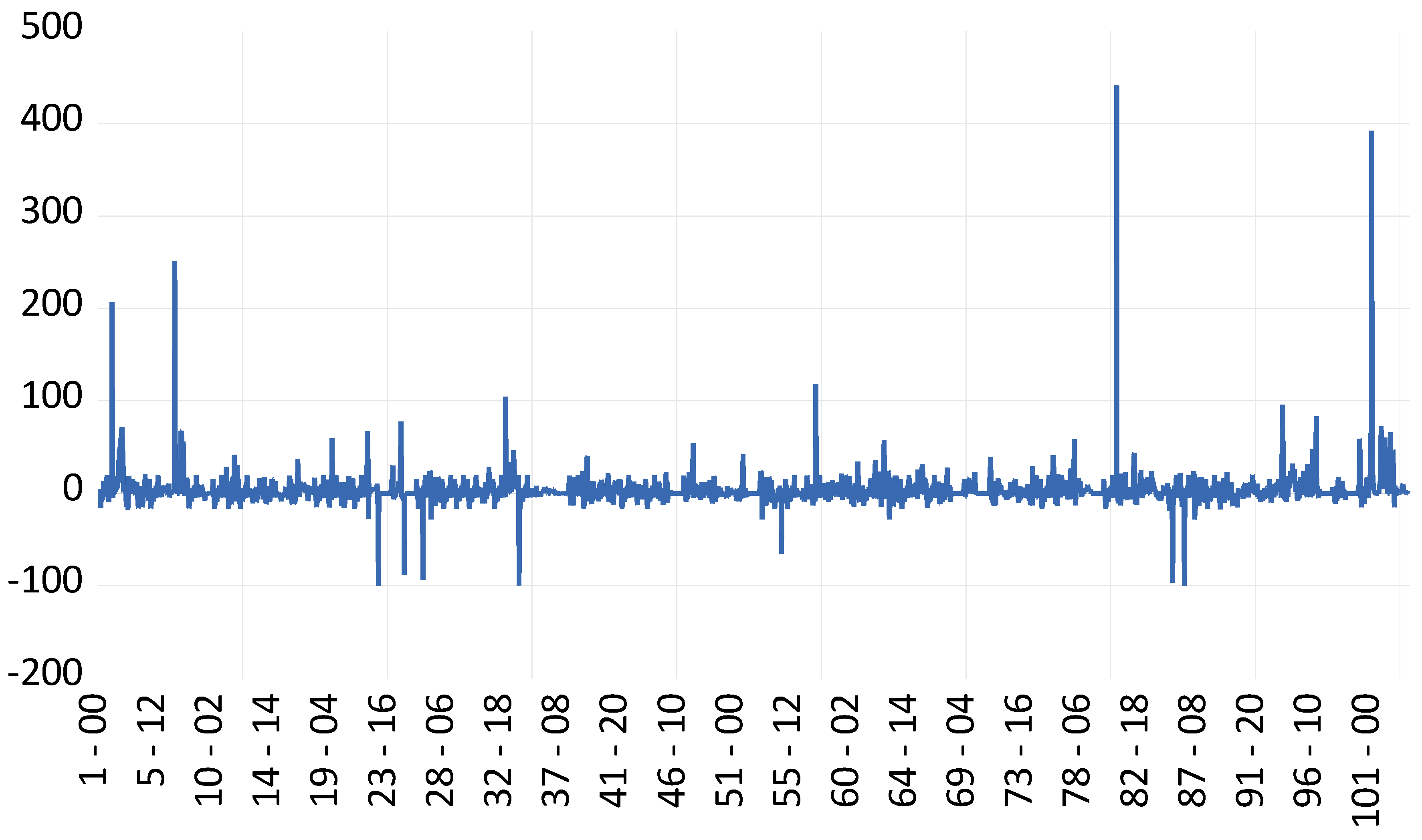
The first step in the analysis is to estimate an exchange rate volatility measure using the EGARCH model. Several previous studies have used this method to measure exchange rate volatility (Oyadeyi, 2026). To do this, the study first plotted the changes in the exchange rate series to establish its volatility. This was depicted in Figure 1. Secondly, to establish its volatility using the EGARCH method, the ordinary least squares (OLS) method was used to estimate the model via the mean equation, as presented in

Table 2. Generalised error distribution.

Variable	Coefficient	Std. Error	z-Statistic	Prob.
C	2.5055	0.4323	5.7957	0.0000
Exc rate changes (−1)	0.2421	0.0400	6.0562	0.0000
	Variance Equation
C	261.4712	4.7131	55.4776	0.0000
RESID(−1)^2	0.3055	0.0135	22.6083	0.0000
EGARCH(−1)	−0.0094	0.0144	−0.6519	0.5145
R-squared	0.0346	Mean dependent var	3.0648
Adjusted R-squared	0.0342	S.D. dependent var	18.9107
S.E. of regression	18.5845	Akaike info criterion	8.5057
Sum squared resid	781,602.2	Schwarz criterion	8.5183
Log likelihood	−9627.7	Hannan–Quinn criterion.	8.5103
Durbin–Watson stat	2.0995
Heteroscedasticity	F-statistic	3.5348	Prob. F(1, 2262)	0.0202 **
Heteroscedasticity	Obs. × R-squared	3.5324	Prob. chi-square(1)	0.0202 **

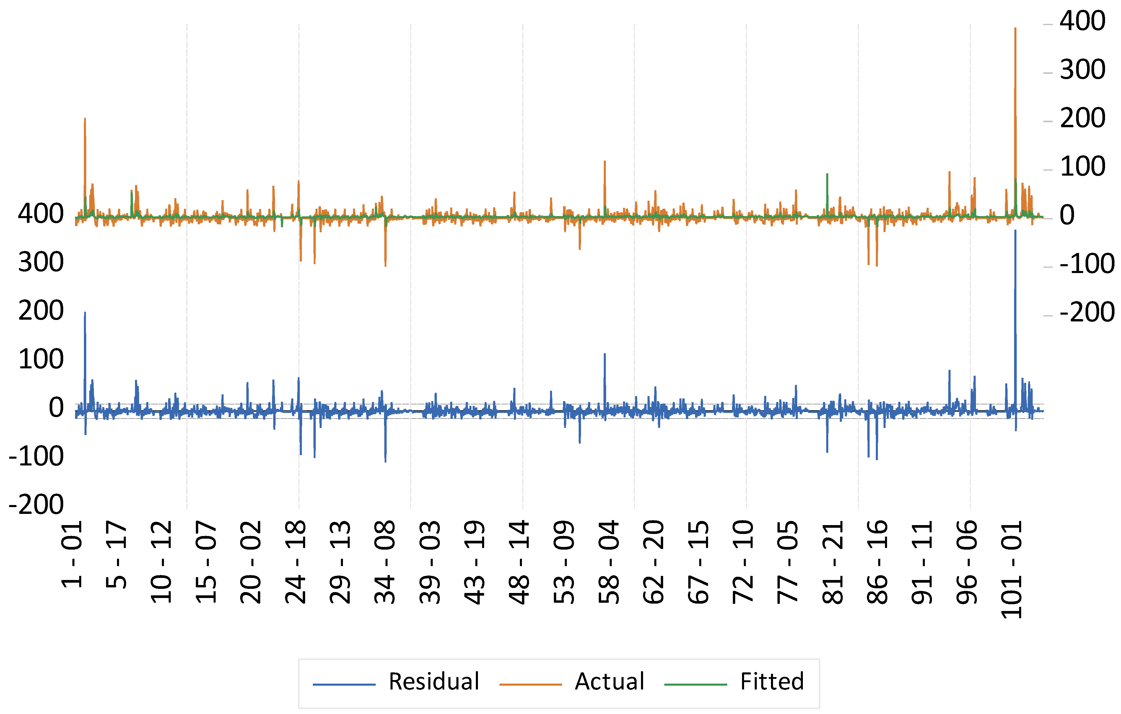
Source: authors’ computation. ** implies significance at 5% level.

. At the same time, the residuals from the OLS model were plotted against the actual and fitted series to assess its performance, as shown in Figure 2. The residual is depicted to illustrate the degree of currency rate fluctuations across countries, and Figure 2 shows that the residual fluctuated during the research period. Therefore, the use of the EGARCH method is reliable and valid, as the residuals are highly volatile, which is the first condition for its application. The second condition can be confirmed by checking the heteroscedasticity test using the Autoregressive Conditional Heteroscedasticity (ARCH) method for the OLS equation estimated. The condition states that the heteroscedasticity test using the ARCH method’s p-value must be less than 0.05 (5% significance level) for the study to use the EGARCH method. The findings in Table 2 indicate that we accept the alternative hypothesis and conclude that the ARCH approach is appropriate for achieving the study’s aims, as its value is significant at the 5% level.

4.2. Pre-Estimation Analysis

After establishing the validity of the EGARCH method, the study proceeds to check the descriptive and multicollinearity properties of the variables used within the models. From

Table 3. Descriptive characteristics of the variables.

Variable	Obs.	Mean	Std. Dev.	Min	Max
ERV	2266	3.07	18.91	−99.99	441.66
Z-score	2266	16.04	9.50	−0.33	66.27
NPL	2266	6.63	7.33	0.10	74.10
Capital	2266	9.75	3.71	1.49	53.50
Credit	2266	106.50	72.90	0.00	898.05
Risk	2266	16.59	4.66	0.88	48.60
Liquidity	2266	34.00	17.40	0.38	145.31
CAT	2266	−1.15	7.88	−40.69	45.46
RGDP	2266	625,000,000,000	1,990,000,000,000	859,000,000	20,900,000,000,000
GEXP	2266	16.42	5.73	0.00	46.26
INF	2266	5.99	12.75	−16.86	254.95

Source: authors’ computation.

, there are 2266 complete observations across the panel datasets, showing that the study used a balanced panel. Moreover, all the datasets were within their minimum and maximum values, showing consistency and reliability. Furthermore, the average exchange rate volatility was 3.07, with a standard deviation of 18.91. The variable with the least mean was the current account balance (% of GDP), while the variable with the highest mean was real GDP. This led us to compute the natural logarithm of the real GDP series before estimating it in the model, since it has the largest mean and deviation from the mean. Additionally, the variable with the least deviation from the mean is government expenditure, while the one with the most significant deviation is real GDP. In essence, the descriptive statistics show that the data exhibit sufficient variation and no obvious anomalies in terms of distribution, suggesting that the dataset is suitable for econometric analysis.

Table 4. Correlation matrix.

	ERV	Z-Score	NPL	Capital	Credit	Risk	Liquidity	CAT	LRGDP	GEXP	INF
ERV	1.0000
Z-score	−0.0233	1.0000
NPL	0.1049	−0.1628	1.0000
Capital	0.1032	−0.0175	0.1610	1.0000
Credit	0.0035	−0.0542	−0.1296	−0.0569	1.0000
Risk	0.0741	−0.0459	0.0954	0.6263	−0.1914	1.0000
Liquidity	0.0282	−0.0185	−0.0433	−0.0096	−0.1006	0.2948	1.0000
CAT	−0.0335	0.0548	−0.1209	−0.1504	0.0613	−0.0594	0.0233	1.0000
RGDP	−0.0334	0.1366	−0.1350	−0.1197	0.0396	−0.1435	−0.0645	0.0514	1.0000
GEXP	−0.0188	−0.0167	−0.1265	−0.0959	0.0502	0.0240	0.1973	−0.0483	0.0156	1.0000
INF	0.1629	−0.0961	0.0622	0.1302	−0.0815	0.0307	0.0181	−0.0609	−0.0683	−0.1236	1.0000

Source: authors’ computation.

presents the correlation matrix for the series and indicates whether multicollinearity exists among the independent variables. The findings suggest that the correlations among the variables were generally weak, and the test for multicollinearity indicates that multicollinearity does not exist among the independent variables, as their correlation matrix is well below 0.8. Therefore, since the correlations are all below the commonly used thresholds, this indicates that multicollinearity is not severe and the independent variables can be reliably included together in the regression model.

Before proceeding to the main analysis, the study further examined cross-sectional dependence (CSD), unit root characteristics of the datasets, slope homogeneity and cointegration tests. The findings of the CSD tests, according to Breusch and Pagan (1980), Pesaran et al. (2008), Baltagi et al. (2012), and Pesaran (2021), presented in

Table 5. Cross-sectional dependence, unit roots, slope homogeneity, and cointegration tests.

	Cross-Sectional Dependence Test				Unit Root Test
Variables	Breusch–Pagan LM	Pesaran Scaled LM	Bias-Corrected Scaled LM	Pesaran CD	CIPS I(0)	CIPS I(1)	CADF I(0)	CADF I(1)
Z-score	19,033.67 ***	134.4472 ***	131.9948 ***	20.126 ***	−2.504 ***		−2.287 ***
LERV	12,987.74 ***	75.46175 ***	73.00937 ***	44.0588 ***	−4.238 ***		−3.799 ***
NPL	26,865.88 ***	210.8598 ***	208.4074 ***	57.061 ***	−2.516 ***		−2.601 ***
Capital	23,497.50 ***	177.9973 ***	175.5449 ***	21.575 ***	−2.253 ***		−2.475 ***
Credit	23,879.30 ***	178.2456 ***	176.4582 ***	21.152 ***	−1.805	−3.784 ***	−1.824	−2.836 ***
Risk	28,183.54 ***	223.7153 ***	221.2629 ***	44.142 ***	−2.145 ***		−1.987 ***
Liquidity	23,724.76 ***	180.2145 ***	177.7621 ***	30.7449 ***	−2.079 ***		−2.135 ***
CAT	22,171.52 ***	163.315 ***	165.4528 ***	12.238 ***	−2.157 ***		−1.955 **
LRGDP	93,842.13 ***	864.2945 ***	861.8421 ***	290.7417 ***	−1.679	−2.928 ***	−1.85	−2.18 ***
GEXP	12,987.93 ***	180.5487 ***	175.8313 ***	47.61 ***	−1.334	−3.65 ***	−1.518	−2.642 ***
INF	20,825.69 ***	151.9305 ***	149.4781 ***	89.1144 ***	−2.602 ***		−2.211 ***
Slope Homogeneity Test	18.311 ***
Cointegration	11.6172 ***

Source: Authors’ computation. Unit root CIPS critical values at 10% (−2), 5% (−2.05), and 1% (−2.14). *** indicates significance at 1% level, while ** indicates significance at 5% level.

, showed that there is evidence of strong CSD among the 103 countries, thereby implying that we reject the null hypothesis of no CSD among the countries since the results are significant at 1%, suggesting that shocks affecting some countries have spillover effects on others within the global dataset. Since CSD was present in the selected countries, the study examined slope homogeneity using Pesaran and Yamagata’s (2008) methods. The table showed that the model’s slope was heterogeneous. This means the model’s slopes differ across the different cross-sectional elements, leading to the rejection of the null hypothesis of slope homogeneity.

Since CSD was present in the datasets, the study utilised cross-sectional unit root tests, including the cross-sectional Im–Pesaran–Shin test and the augmented Dickey–Fuller test that accounts for cross-sectional dependence. The findings showed that, apart from credit, real GDP and government expenditure, all other variables were stationary in their level form. In contrast, credit, real GDP, and government expenditure were stationary in their first differences. Due to these findings, the study employed cointegration tests using Westerlund’s (2007) method. The findings, presented in Table 5, also revealed a long-run relationship within the model. Therefore, the results of the CSD, slope homogeneity, and cointegration tests suggest using appropriate robust estimators such as D-K and the two-step system GMM methods.

4.3. Main Analysis

Table 6. Main results and sensitivity of the results.

	Main Analysis	Robustness	Sensitivity Using Quantile Regressions
VARIABLES	Driscroll–Kraay	Two-Step GMM	Location	Scale	Q = 10	Q = 25	Q = 50	Q = 75	Q = 90
LERV	−0.533 **	−0.5038 *	−0.1675 **	−0.1754 ***	−0.1567 ***	−0.1601 ***	−0.1662 ***	−0.1717 ***	−0.1805 ***
	(0.2010)	(0.2983)	(0.0662)	(0.0566)	(0.0560)	(0.0458)	(0.0595)	(0.0518)	(0.0157)
NPL	−0.2439 ***	−0.248 ***	−0.238 ***	−0.114 ***	−0.0745 ***	−0.126 ***	−0.219 ***	−0.302 ***	−0.435 ***
	(0.0220)	(0.0893)	(0.0256)	(0.0219)	(0.0215)	(0.0177)	(0.0228)	(0.0352)	(0.0587)
Capital	0.477 ***	0.257 ***	0.146 *	0.1869 **	0.1213 *	0.1608 ***	0.161 ***	0.194 ***	0.296 ***
	(0.0703)	(0.0700)	(0.0865)	(0.074)	(0.0731)	(0.0598)	(0.0177)	(0.012)	(0.0200)
D.Credit	0.0127 ***	0.0765 *	0.0122 ***	0.0195 ***	0.0136 ***	0.0143 ***	0.0518 ***	0.0533 ***	0.0555 **
	(0.0019)	(0.0453)	(0.00312)	(0.0027)	(0.0026)	(0.0022)	(0.0028)	(0.0043)	(0.0072)
Risk	−0.230 ***	−0.217 ***	−0.205 ***	−0.153 ***	−0.0157 ***	−0.0541 ***	−0.178 ***	−0.290 ***	−0.469 ***
	(0.0493)	(0.0186)	(0.0668)	(0.0572)	(0.0056)	(0.0046)	(0.0599)	(0.0925)	(0.154)
Liquidity	0.0345 **	0.130 ***	0.1230 ***	0.1622 ***	0.1077 ***	0.1487 ***	0.1570 ***	0.1647 ***	0.1719 ***
	(0.0136)	(0.0352)	(0.0142)	(0.0121)	(0.012)	(0.0098)	(0.0127)	(0.0197)	(0.0327)
CAT	0.0453 **	0.0519 ***	0.0690 **	0.1901 ***	0.0965 ***	0.0878 ***	0.0723 **	0.0584 ***	0.0361 **
	(0.0163)	(0.0106)	(0.0318)	(0.0272)	(0.0269)	(0.022)	(0.0285)	(0.0144)	(0.0173)
D.LRGDP	0.2752 ***	0.2863 ***	0.419 ***	0.357 ***	0.0942 ***	0.0983 ***	0.357 ***	0.4618 **	0.5035 ***
	(0.0185)	(0.0148)	(0.147)	(0.126)	(0.0124)	(0.0101)	(0.131)	(0.203)	(0.0338)
D.GEXP	−0.212 ***	−0.285 ***	−0.0669 ***	−0.0782 **	−0.0931 **	−0.0848 ***	−0.0701 *	−0.0568 ***	−0.0356 ***
	(0.0633)	(0.0619)	(0.0236)	(0.0373)	(0.0369)	(0.0302)	(0.0391)	(0.0205)	(0.0101)
INF	−0.0648 ***	−0.0524 ***	−0.0709 ***	−0.5125 ***	−0.0529 ***	−0.0586 ***	−0.0687 ***	−0.0778 ***	−0.0924 ***
	(0.0055)	(0.0036)	(0.0154)	(0.0132)	(0.013)	(0.0107)	(0.0138)	(0.0214)	(0.0356)
Constant	0.5844 ***	0.4712 ***	0.4267 ***	0.1897 ***	0.1543 ***	0.2405 ***	0.3940 ***	0.5324 ***	0.7534 ***
	(0.1250)	(0.1724)	(0.0561)	(0.0481)	(0.0479)	(0.0387)	(0.0522)	(0.0775)	(0.1291)
Observations	2266	2266	2266	2266	2266	2266	2266	2266	2266
Number of groups	103	103	103	103	103	103	103	103	103
AR(1)		0.0152
AR(2)		0.1160
Sargan test		0.4523
Hansen test		0.5687
F(10, 102)	438.84 ***	38.71 ***
No. of instruments		241

Source: authors’ computation. For the Driscoll–Kraay and two-step system GMM results, standard errors are in parentheses. For the quantile regression results, z-statistics are in parentheses. *** p < 0.01, ** p < 0.05, * p < 0.1.

presents the main findings of the study. It examines the effects of exchange rate volatility on corporate financial stability across the 103 countries in the regression. To achieve this, the Driscoll and Kraay (1998) fixed-effect estimator was used to obtain the findings, while the study employed the two-step system GMM method for triangulation. The Driscoll–Kraay results showed that exchange rate volatility adversely affected financial stability by roughly 53%. This suggests that policies or shocks that increase currency volatility tend to heighten financial instability or weaken financial stability. The findings of adverse exchange rate volatility effects on financial stability align with previous studies by Coudert et al. (2011), Kasman et al. (2011), Blau (2018), Athari et al. (2023), and Agénor et al. (2026).

Furthermore, the findings from the bank-level characteristics revealed that bank capital, bank credit, and bank liquidity are positive sources of financial stability. This implies that a rise in bank capital, bank credit and bank liquidity would improve financial stability across these countries. The findings of a positive effect of bank capital on financial stability align with previous studies like Lepetit et al. (2008), Berger et al. (2009), and Anginer et al. (2014), while the findings of a positive impact of bank liquidity on financial stability align with studies like Distinguin et al. (2013), Gupta et al. (2023) and Población García and Suárez (2025). Again, the positive findings regarding bank credit align with studies by Beck et al. (2013b), Andrieş and Căpraru (2014), and Jiménez et al. (2017). On the other hand, a rise in financial risks and non-performing loans will weaken financial stability, as the coefficients for these variables are negative. This suggests that higher financial risks and non-performing loans are causes of financial instability worldwide, as they negatively affect financial stability within the model. These findings align with previous studies, including Serrano (2021), Bacchiocchi et al. (2022), and Atichasari et al. (2023).

For the macroeconomic variables within the model, the findings from Table 6 suggest that real GDP and the current account have positive effects on financial stability. This indicates that the higher the real GDP and the current account balance, the greater the level of financial stability in an economy. Therefore, this suggests that when the real and external sectors are performing well, they tend to positively influence financial stability in the selected countries. These findings align with previous studies, including Altayligil and Çetrez (2020) and Mabkhot and Al-Wesabi (2022). On the other hand, the findings showed that a higher inflation rate and government expenditure tend to reduce financial stability. This is due to the negative coefficients of these variables. These findings suggest that when there are price pressures and when government spending is very high, they tend to exacerbate instability within the financial system. These findings are similar to findings by Boyd et al. (2001) and Ullah et al. (2024), in their studies.

While the findings on inflation seem to follow a priori, the findings on government spending suggest two things. First, government spending may not be targeted at productive investments, thereby weakening fiscal imbalances, escalating public debt and leading to inefficient allocation and use of public resources, especially when the composition of government spending is skewed toward less productive expenditures (Alesina et al., 2019). Excessive recurrent expenditure relative to capital expenditure can lead to poorly planned fiscal policy implementation, displacing private investment, elevating borrowing costs, and generating uncertainty for financial institutions. Second, a rise in government spending may increase macroeconomic pressures, such as inflation or currency depreciation, especially in countries with fiscal discipline issues. These pressures can lead to a decline in bank assets, deterioration in credit quality, and may undermine trust within the financial system. Banks may subsequently witness higher non-performing loans and heightened risk exposure, thereby exacerbating financial instability.

The second model in Table 6 showcased the same results using the two-step system GMM procedure. While the D-K estimators have helped correct for cross-sectional dependence, serial correlation, and heteroscedasticity, they do not correct for endogeneity. The two-step system GMM helps correct for endogeneity, captures dynamic persistence and accounts for measurement errors (Arellano & Bover, 1995; Blundell & Bond, 1998; Roodman, 2009). Therefore, the two-step system GMM estimator was employed to improve the credibility and robustness of the main findings. The findings were in line with the main findings using the D-K method, showing that the primary findings were credible, valid and reliable in the presence of another estimation technique. Additionally, the tests for serial correlation using the AR(2) p-values show that they are consistently above 0.05, indicating that we fail to reject the null hypothesis of no second-order serial correlation in the differenced residuals. This outcome confirms that the model is correctly specified and satisfies a key requirement for the validity of the dynamic panel estimator.

In summary, the findings of the study align clearly with the financial accelerator theory (the theoretical foundation of the study), as the findings show that shocks have consequential effects on financial stability. This finding is further supported by the financial accelerator theory’s unique ability to explain how exchange rate volatility affects financial stability, especially in countries where banks have greater exposure to currency risks. The financial accelerator theory posits that external shocks, whether small or large, may amplify effects on real economic activity, particularly when they operate through the balance sheets of banks and borrowers. As a result, the findings of the study align with the financial accelerator theory, indicating that external shocks, such as exchange rate volatility, have consequential effects on financial stability. Therefore, the theory provides evidence that macroeconomic conditions and shocks are harmful and weaken the effects of currency volatility on bank stability.

4.4. Sensitivity Results Using Quantile Regressions

To assess the sensitivity of the main findings, the study employed quantile regressions to examine their robustness across different quantiles. The findings, also in Table 6, revealed varying impacts of the independent variables on financial stability across the different points in the distribution. To start, exchange rate volatility generally demonstrates a negative and significant effect on financial stability, reducing their average level (−0.1675 **) and variability (−0.1754 ***). Moreover, the impact is quantile-dependent as it has a more pronounced impact on financial stability at the upper end of the distribution (Q = 0.75, Q = 0.9) than it has at the lower end or median point of the distribution (Q = 0.1, Q = 0.25, Q = 0.5). These suggest that countries at the top end of the stability distribution experience slightly larger and more disruptive effects from currency shocks, while weaker countries are affected less because they are already close to instability thresholds.

Furthermore, bank capital, bank credit and bank liquidity also showed that their impact on financial stability is quantile-dependent as they are more pronounced at the upper end of the distribution where Q = 0.75 (−0.1717) and Q = 0.9 (−0.1805) than the lower end of the distribution Q = 0.1 (−0.1567), Q = 0.25 (−0.1601), and Q = 0.5 (−0.1662). These suggest that countries at the top end of stability distribution, that is, banks in more stable environments, can convert additional lending into greater resilience and stability. This is possible due to stronger capital buffers, better credit management frameworks, and stronger bank liquidity management. On the other hand, banks in the lower quantile of the distribution showed that bank capital, liquidity, and credit have smaller effects. This means that fragile banking systems may not be able to translate additional capital, credit management, and liquidity management into greater resilience compared to banks in stronger, more advanced environments.

Regarding bank non-performing loans and risk exposure, the findings also showed that stronger banking systems are more sensitive to higher levels of non-performing loans and risks. For instance, more stable banks in the upper quantile experience a larger decline in financial stability when their NLPs or risk exposure rise. This indicates that a decline in asset quality or an increase in risk exposure may cause banking systems at the upper echelons to lose financial stability swiftly. Therefore, they must maintain low levels of NPLs to preserve their stability. On the other hand, banks at the lower end of the quantile distribution are shown to be already constrained by fragile banking systems. Therefore, they experience less decline compared to those at the upper end of the distribution when NPLs and risk exposure rise, since they operate at levels close to distress conditions. Consequently, subsequent shocks to these systems have less marginal impact on their vulnerability, meaning that weaker banking systems have little room before they approach crisis thresholds.

Regarding macroeconomic conditions, the quantile regression findings suggest that stronger economies experience greater stability from external balance and economic growth than weaker economies. This is because their effects are larger across the higher quantiles. Therefore, countries with stronger stability conditions benefit more from growth and healthier positions than those with weaker stability conditions at the lower end of the quantile. On the other hand, the findings from the inflation rate reveal that countries in the upper quantiles have more stable banking systems, deeper financial markets, and wider credit exposure, and a higher inflation reduces real returns, increases credit risk and weakens liquidity more rapidly in these environments. This can lead to sharper declines in financial stability than in countries with a lower distribution of quantiles. Therefore, countries at the lower distribution also experience financial instability, but this is a marginally lower level compared to those at the upper distribution since many countries at the lower distribution are already constrained by instability issues. Therefore, inflation has more debilitating consequences in countries with more stable financial systems than those with weaker systems. Finally, because government expenditure has a smaller effect on the upper quantile of the distribution than on the lower, this suggests that fragile financial systems are more prone to being hurt by rising government expenditure than stable financial systems. This may be due to inefficiency in government spending, weaker institutions and poorer fiscal management compared to more stable environments.

4.5. Analysis Based on Country Income Classification

The analysis based on countries’ income classifications is presented in

Table 7. Robustness results grouping countries by their income level.

	Driscoll–Kraay Results					Two-Step System GMM Results
VARIABLES	HIC	UMIC	MIC	LMIC	LIC	HIC	UMIC	MIC	LMIC	LIC
LERV	−0.2489 ***	−0.2787 ***	−0.2767 ***	−0.2716 ***	−0.2753 ***	−0.346 ***	−0.4013 ***	−0.1355 ***	0.0516 ***	0.01456 ***
	(0.0681)	(0.0919)	(0.0786)	(0.0910)	(0.0231)	(0.0266)	(0.0395)	(0.0238)	(0.0192)	(0.0346)
NPL	−0.438 ***	−0.303 ***	−0.154 ***	−0.0961 *	−0.4430 ***	−0.438 ***	−0.188 ***	−0.164 ***	−0.120 ***	0.4345 ***
	(0.0462)	(0.0279)	(0.0291)	(0.0512)	(0.0285)	(0.155)	(0.0173)	(0.0110)	(0.0113)	(0.0298)
Capital	0.473 ***	0.385 **	0.146 ***	0.702 ***	0.707 *	0.352 ***	0.304 ***	0.790 **	0.796 *	0.234 ***
	(0.161)	(0.177)	(0.0162)	(0.208)	(0.402)	(0.0615)	(0.0364)	(0.358)	(0.444)	(0.0267)
D.Credit	0.1840 ***	0.0805 ***	0.0374 ***	0.0815 ***	0.182 *	0.0827 ***	0.1040 *	0.0911 **	0.1301 ***	0.1238 ***
	(0.0388)	(0.0083)	(0.0066)	(0.0127)	(0.094)	(0.0239)	(0.0541)	(0.043)	(0.0391)	(0.0021)
Risk	−0.126 ***	−0.1981 ***	−0.199 ***	−0.1886 ***	−0.430 ***	−0.0518 **	−0.1468 ***	−0.321 ***	−0.068 ***	0.414 ***
	(0.0174)	(0.0133)	(0.0142)	(0.0202)	(0.104)	(0.0241)	(0.0234)	(0.0324)	(0.0240)	(0.0177)
Liquidity	0.0527 **	0.1274 ***	0.0247 **	0.1008 ***	0.178 ***	0.1537 ***	0.1077 ***	0.175 ***	0.1268 **	0.1715 ***
	(0.024)	(0.0166)	(0.0092)	(0.0248)	(0.0176)	(0.0555)	(0.0542)	(0.0475)	(0.0616)	(0.0463)
CAT	0.151 ***	0.288 ***	0.257 ***	0.202 ***	0.283 ***	0.195 ***	0.211 ***	0.272 **	0.171 **	0.242 ***
	(0.0249)	(0.101)	(0.063)	(0.0437)	(0.0475)	(0.0158)	(0.0247)	(0.132)	(0.0753)	(0.079)
D.LRGDP	0.5735 ***	0.1578 ***	0.1656 ***	0.3553 ***	0.3316 ***	0.5745 ***	0.3231 **	0.1174 ***	0.4128 ***	0.1378 ***
	(0.1128)	(0.0346)	(0.0422)	(0.0689)	(0.1026)	(0.0189)	(0.1333)	(0.0025)	(0.1304)	(0.0129)
D.GEXP	−0.417 **	−0.461 ***	−0.345 *	−0.757 ***	−0.489 ***	−0.293 ***	−0.478 ***	−0.328 **	−0.809 **	−0.488 ***
	(0.188)	(0.0300)	(0.168)	(0.188)	(0.133)	(0.0606)	(0.0934)	(0.146)	(0.408)	(0.0198)
INF	−0.262 **	−0.0485 ***	−0.0648 ***	−0.205 **	−0.367 ***	−0.325 ***	−0.2950 ***	−0.1762 ***	−0.213 **	−0.364 ***
	(0.115)	(0.013)	(0.0181)	(0.084)	(0.0798)	(0.0264)	(0.0366)	(0.0598)	(0.0863)	(0.0821)
Constant	0.2664 ***	0.2544 ***	0.2834 ***	0.2878 ***	0.4089 ***	0.1449 ***	0.4315 ***	0.3281 ***	0.2860 **	0.3897 ***
	(0.0993)	(0.0642)	(0.0559)	(0.0571)	(0.1366)	(0.0159)	(0.0248)	(0.0146)	(0.1155)	(0.0498)
Observations	1012	682	1116	484	88	1012	682	1116	484	88
No. of countries	46	31	53	22	4	46	31	53	22	4
AR(1)						0.153	0.195	0.144	0.131	0.171
AR(2)						0.135	0.642	0.298	0.392	0.539
Sargan test						0.1986	0.1987	0.1967	0.1378	0.1897
Hansen test						0.2345	0.2127	0.2378	0.2347	0.2126
F(10, 102)						14.43	19.95	21.86	92	12.71
No. of instruments						241	241	241	241	81

Source: authors’ computation. Standard errors are in parentheses for the Driscoll–Kraay and two-step system GMM results. *** p < 0.01, ** p < 0.05, * p < 0.1. HIC represents high-income countries; UMIC represents upper-middle-income countries; MIC represents middle-income countries; LMIC represents lower-middle-income countries; and LIC represents low-income countries.

. It focuses on dividing countries by income level and on whether the findings remain consistent with the study’s primary findings. The findings are aligned with the primary findings of the study using both the D-K method and the two-step GMM method, indicating that our results were robust despite the study’s income-group division. Therefore, exchange rate volatility has a negative effect on financial stability, while bank-level factors, such as capital and liquidity, are sources of stability, whereas higher non-performing loans and risks are sources of instability. On the other hand, macroeconomic factors such as positive real GDP growth and a positive current account balance are sources of financial stability, while a higher inflation rate and government expenditure are sources of financial instability across the selected countries.

4.6. The Effects of Economic Policy Uncertainty and Institutional Quality Within the Model

Economic policy uncertainty (EPU) and institutional quality are two important determinants of financial stability based on the past literature. As a result, the study sought to establish this relationship since several studies have shown mixed effects on the effects of institutional quality and EPU on financial stability. As a result, the study analyses the effects of EPU and the six institutional quality variables (voice and accountability, political stability, government effectiveness, rule of law, regulatory quality and control of corruption) on financial stability across the selected countries. Moreover, the study considered the six institutional quality indicators separately since it is assumed that, for instance, the way regulatory quality will affect financial stability is different from the way the control of corruption and political stability will affect financial stability. This results in seven model specifications, including one baseline model and six additional models incorporating each institutional indicator separately. This approach is important as it allows the study to identify the distinct contribution of each governance dimension to financial stability. Therefore, the findings from

Table 8. The effects of economic policy uncertainty and institutional quality on financial stability.

	Model 1	Model 2	Model 3	Model 4	Model 5	Model 6	Model 7
VARIABLES	Economic Policy Uncertainty	Voice and Accountability	Political Stability	Government Effectiveness	Regulatory Quality	Rule of Law	Control of Corruption
LERV	−1.563 **	−1.536 *	−1.706 **	−1.589 *	−1.660 **	−1.692 **	−1.677 **
	(0.790)	(0.797)	(0.818)	(0.814)	(0.827)	(0.785)	(0.828)
Economic Policy Uncertainty	−0.0121 ***
	(0.0027)
Voice and Accountability		2.102 ***
		(0.335)
Political Stability			1.225 ***
			(0.411)
Government Effectiveness				1.510 ***
				(0.347)
Regulatory Quality					1.234 ***
					(0.381)
Rule of Law						0.950 ***
						(0.243)
Corruption Control							0.519 ***
							(0.182)
NPL	−0.215 ***	−0.280 ***	−0.220 ***	−0.221 ***	−0.214 ***	−0.215 ***	−0.224 ***
	(0.0489)	(0.0338)	(0.0546)	(0.0448)	(0.0458)	(0.0525)	(0.0502)
Capital	0.201 **	0.2367 ***	0.200 **	0.1964 **	0.219 **	0.224 ***	0.222 ***
	(0.0741)	(0.0834)	(0.0795)	(0.0814)	(0.0827)	(0.0734)	(0.0748)
D.Credit	0.1528 ***	0.1220 ***	0.0766 ***	0.0797 ***	0.0696 ***	0.0809 ***	0.0773 ***
	(0.0127)	(0.013)	(0.0131)	(0.0132)	(0.0137)	(0.0123)	(0.0129)
Risk	−0.205 *	−0.100 ***	−0.169 *	−0.104 ***	−0.113 ***	−0.184 *	−0.181 *
	(0.1070)	(0.0330)	(0.0947)	(0.0278)	(0.0118)	(0.1040)	(0.1020)
Liquidity	0.0319 **	0.0308 **	0.0401 **	0.0398 **	0.0385 **	0.0878 ***	0.0377 ***
	(0.0144)	(0.0154)	(0.0155)	(0.0153)	(0.0152)	(0.0149)	(0.0142)
CAT	0.0439 *	0.0568 **	0.0576 **	0.0516 *	0.0496 *	0.0549 **	0.0549 **
	(0.0221)	(0.0271)	(0.0276)	(0.0266)	(0.0286)	(0.0245)	(0.0216)
D.LRGDP	0.6890 **	0.793 ***	0.5321 ***	0.3069 *	0.3030 **	0.2879 **	0.2752 **
	(0.2723)	(0.2917)	(0.1939)	(0.1782)	(0.1413)	(0.1389)	(0.1139)
D.GEXP	−0.326 **	−0.385 ***	−0.286 **	−0.365 **	−0.335 **	−0.273 *	−0.278 **
	(0.1520)	(0.1320)	(0.1330)	(0.1440)	(0.1380)	(0.1350)	(0.1300)
INF	−0.0615 ***	−0.0929 ***	−0.0612 ***	−0.0757 ***	−0.0708 ***	−0.0601 ***	−0.0587 ***
	(0.0136)	(0.0229)	(0.0135)	(0.0151)	(0.0142)	(0.0131)	(0.0143)
Constant	26.17 ***	29.53 ***	28.38 ***	28.00 ***	28.15 ***	28.38 ***	28.20 ***
	(5.1630)	(4.8780)	(5.4680)	(5.3190)	(5.4410)	(5.3920)	(5.5990)
Observations	2266	2266	2266	2266	2266	2266	2266
R-squared	0.5	0.73	0.46	0.67	0.59	0.54	0.48
Number of groups	103	103	103	103	103	103	103

Source: authors’ computation. Standard errors are in parentheses for the Driscoll–Kraay results. ***, **, and * are the significance of the results at 1%, 5%, and 10% respectively.

show that the effects of exchange rate volatility and the other bank-level and macro-level variables remain the same across the seven different models, thereby supporting the initial findings and strengthening the conclusions of the study.

On the other hand, EPU (−0.0121) has negative effects on financial stability across the selected countries. This suggests that financial stability declines as policy uncertainty rises or that increases in policy uncertainty reduce financial stability. This is important as it suggests that uncertainty in economic policy weakens confidence, increases risk perception, and transmits instability to the banking sector. Practically speaking, this implies that financial systems become more brittle, volatile, and risk-prone when economic policies are unexpected. These findings on the effects of EPU on stability align with previous studies by Oyadeyi (2025) and Oyadeyi et al. (2026). On the other hand, all six institutional quality indicators have positive effects on financial stability across the selected sample. These indicate that a comprehensive governance framework across all six indicators is a strong condition for financial stability. Moreover, these institutional frameworks function as a complementary system that lowers systemic risk, improves regulatory effectiveness, and boosts market confidence, thereby holistically driving financial stability. Based on these findings, financial stability is best achieved through broad-based institutional reform, not selective improvements. As a result, improving only regulatory quality without reducing corruption will only have a limited effect on financial stability. Furthermore, strengthening the rule of law without political stability will only lead to incomplete gains. Therefore, the institutional quality reforms must be system-wide, coordinated, and cut-across the six indicators for it to have the desired impact on financial stability across the selected countries.

4.7. Margin Analysis

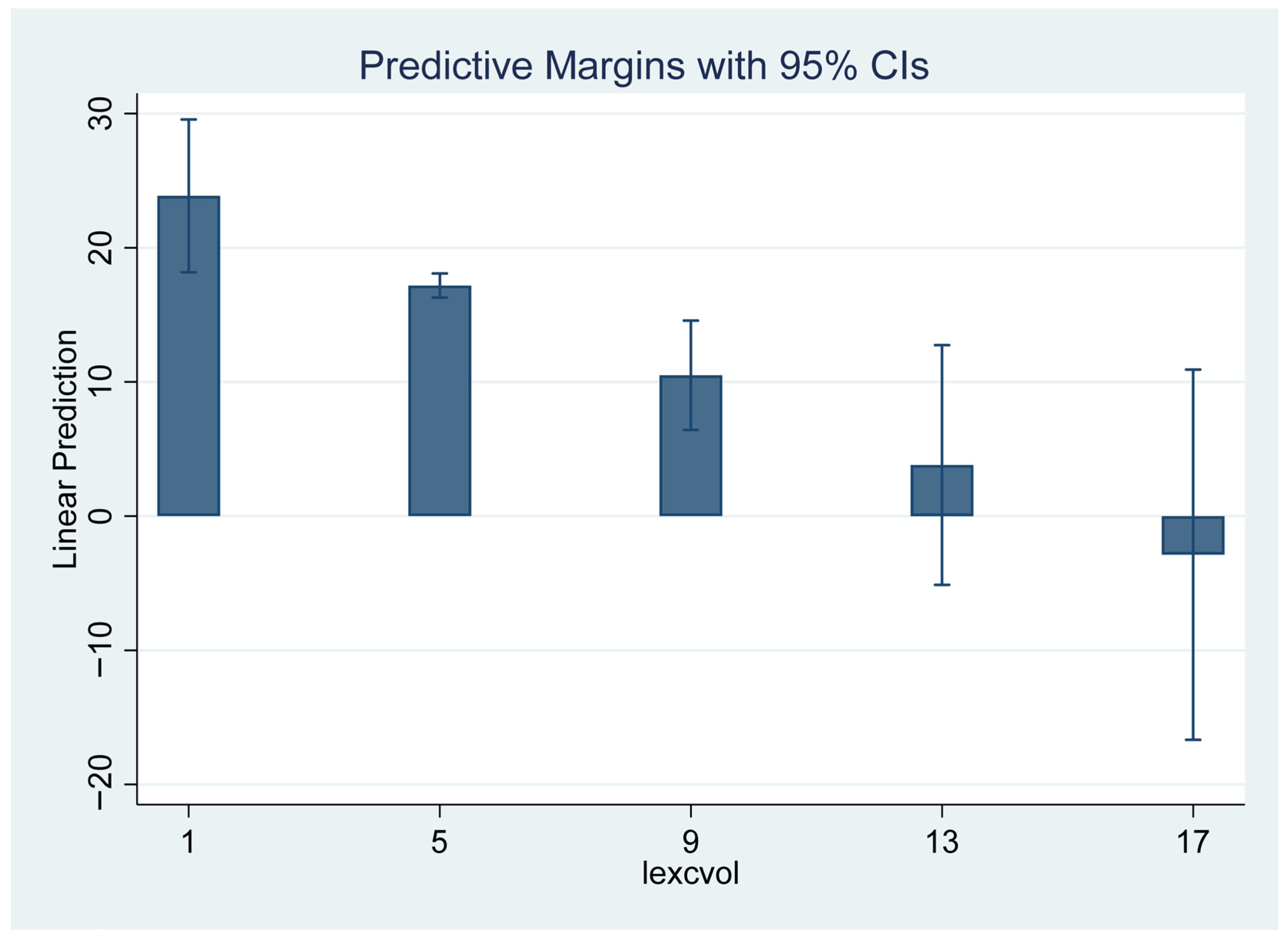
The margin analysis constitutes the final analysis of the study. It provides evidence on the expected financial stability impact from exchange rate volatility, based on margins. From Figure 3, at 1% exchange rate volatility, the predicted margin in financial stability is 23%. This suggests a higher level of financial stability when exchange rate volatility is very low. On the other hand, when exchange rate volatility increases to 6%, the predicted margin for financial stability is 15.5%, while when exchange rate volatility changes by 10%, the predicted margin for financial stability reduces to 7.2%. Finally, when exchange rate volatility changes by 16%, the predicted financial stability margins fall to a negative value (−1.2%). This suggests that as exchange rate volatility rises, it has debilitating consequences for financial stability, meaning that the point when exchange rate volatility has predicted negative consequences for financial stability is at 16%, leading to a predicted reduction of −1.2% in financial stability. Therefore, the financial system deteriorates, becomes more precarious, and is more susceptible to shocks as currency swings intensify.

5. Conclusions, Recommendations and Limitations

5.1. Summary and Conclusions

The study examined the effects of exchange rate volatility on corporate financial stability across 103 countries worldwide. The countries cut across different regions, including North America, Latin America and the Caribbean, Europe, the Middle East, Sub-Saharan Africa, and Asia. Across income classifications, the selected countries include high-income, middle-income (upper-middle-income and lower-middle-income), and low-income countries. Annual data for 103 countries were collated from 2000 to 2021. The study was limited to 2021 due to the availability of financial variables from the World Bank’s Global Financial Database through 2021. Econometric methods, such as Driscoll and Kraay fixed effects, two-step system GMM, and quantile regressions, were used to achieve the study’s broad objectives.

The study’s findings revealed that exchange rate volatility has significant negative effects on corporate financial stability, whereas financial variables such as bank capital, bank credit, and bank liquidity have positive effects. On the other hand, bank risks and non-performing loans negatively affect financial stability. From the macroeconomic variables, real GDP and the current account have positive effects on financial stability, while government expenditure and inflation have negative effects on corporate financial stability. Additionally, institutional quality has positive effects on financial stability, while economic policy uncertainty has a negative effect on financial stability across the selected countries. Therefore, the study concludes that the findings from this study provide evidence that macroeconomic conditions and shocks are harmful and weaken the effects of exchange rate volatility on financial stability, aligning with the financial accelerator theory.

5.2. Recommendations

Based on the above findings, the study proposes the following policy recommendations. First, when exchange rate volatility jeopardises financial stability, policy responses must prioritise mitigating balance-sheet vulnerabilities stemming from foreign-currency exposure. Regulators ought to enhance macroprudential regulations that restrict unhedged foreign-currency borrowing, impose stricter limits on banks’ net open foreign-exchange positions, and implement elevated risk weights or provisioning requirements for foreign-currency loans granted to borrowers lacking natural hedges. These strategies mitigate currency mismatches and diminish the exacerbation of exchange rate shocks via bank and company balance sheets. Moreover, foreign-currency intervention may be used judiciously and openly to rectify tumultuous market circumstances, especially in countries characterised by shallow foreign-exchange markets and significant dollarisation. These initiatives should augment, rather than replace, effective monetary and macroprudential policy.

Second, enhancing the resilience of the banking industry is equally vital as financial risks rise. Regulatory bodies must guarantee that financial institutions maintain sufficient capital and liquidity reserves to withstand shocks from currency fluctuations and declining asset quality. In areas with heightened vulnerabilities, authorities may consider raising tier II capital requirements, limiting dividend payments, and strengthening liquidity risk management, particularly for foreign-currency financing. Macroprudential instruments, including countercyclical capital buffers, systemic risk buffers, and borrower-based measures, may be used to curtail excessive risk-taking and mitigate procyclicality in credit markets. These strategies augment banks’ capacity to absorb losses and mitigate the risk that localised shocks will evolve into systemic instability.

Third, mitigating the buildup of non-performing loans is crucial for reinstating financial stability and maintaining credit intermediation. Supervisors must implement prompt loan categorisation, uniform definitions of non-performing exposures, and pragmatic provisioning rules to avert the obfuscation of credit risk via loan evergreening. Banks must be mandated to formulate realistic plans for reducing NPLs, underpinned by robust governance, transparent reporting, and adequate write-off policies. Simultaneously, enhancing insolvency regimes, collateral enforcement mechanisms, and secondary markets for distressed assets may expedite balance-sheet rehabilitation. In cases of enduring market failures, the creation of asset management businesses or centralised workout platforms may help systematically resolve distressed assets.

Fourth, when bank capital, credit, and liquidity positively influence financial stability, policy initiatives should prioritise the enhancement and maintenance of these stabilising mechanisms via judicious regulatory and supervisory frameworks. Regulators must persist in implementing stringent capital adequacy standards, including countercyclical and systemic risk buffers, to ensure that banks maintain sufficient loss-absorbing capacity throughout the economic cycle. Simultaneously, policies must facilitate sustainable credit growth, especially in productive economic sectors, while mitigating excessive risk-taking via robust credit rules and borrower-centric macroprudential instruments. Maintaining sufficient liquidity buffers is crucial, since high-quality liquid assets bolster banks’ resilience to financing shocks and reduce the probability of suffering during market turmoil. A comprehensive regulatory framework that fosters robust bank capitalisation, effective loan intermediation, and prudent liquidity management may bolster the banking system’s resilience, reinforce trust, and sustain long-term financial stability without compromising economic growth and development.

In addition, the study’s conclusions indicate that macroprudential rules are crucial for reducing systemic risks and building resilience. In particular, financial stability resilience can be significantly increased by implementing strategies like dynamic provisioning on foreign-currency exposures, prudential guidelines and limits, and countercyclical capital buffers. This will lessen balance-sheet vulnerabilities and excessive risk-taking during times of increased economic policy uncertainty. More significantly, the quality of institutions has a direct impact on how well these policies work, since better governance frameworks promote the legitimacy, coordination, and execution of policies, which in turn support macroprudential regulations and a robust financial system.

Finally, effective policy responses need robust coordination among monetary, fiscal, and macroprudential authorities. Monetary policy must focus on stabilising inflation expectations, whilst macroprudential measures should mitigate systemic financial risks, and foreign-exchange instruments should rectify market inefficiencies and address balance-sheet weaknesses. This cohesive policy strategy ensures that actions in one area do not unintentionally exacerbate risks in another. Enhancing financial safety nets, such as lender-of-last-resort mechanisms, deposit insurance systems, and foreign-currency liquidity support, bolsters trust and crisis readiness. Collectively, these synchronised actions bolster a more robust financial sector, better able to withstand exchange rate fluctuations, heightened banking risks, and rising non-performing loans.

5.3. Limitations and Options for Future Research

The study’s limitation is that data on the financial variables are only available through 2021. It would have been interesting to see whether data in recent years, especially between 2022 and 2025, would have any changes on the findings of the study, especially because recent events such as growing economic uncertainty (including the trade policy from the US) and geopolitics (including Russia’s war on Ukraine and other geopolitical events) may pose significant effects on the results. Therefore, future studies should consider this recent information and re-estimate these results when data on the financial indicators becomes available. This would further establish how exchange rate volatility impacts corporate financial stability in recent times.