The Effects of Financial Stability, Economic Growth, and Industrial Production on Environmental Performance: Evidence from Türkiye

Abstract

Environmental performance constitutes a core dimension of the environmental, social, and governance (ESG) framework; however, empirical evidence for developing economies such as Türkiye remains limited, particularly regarding regime-dependent effects. Accordingly, this study examines the effects of financial stability, economic growth, and industrial production on environmental performance for Türkiye within a Markov-switching error correction and time-varying parameter state–space framework using annual data for 1990–2023. The findings show that financial stability is insignificant in the low error-variance regime but is negatively associated with environmental performance in the high error-variance regime. Economic growth is negatively associated with environmental performance in the low error-variance regime and becomes insignificant in the high error-variance regime. In contrast, industrial production has a positive and statistically significant effect on environmental performance in both regimes. The error correction mechanism indicates that short-run disequilibria are gradually corrected, supporting the existence of long-run convergence. Furthermore, the time-varying parameter state–space estimates indicate that these effects change over time. Overall, the findings indicate that the effects of financial stability, economic growth, and industrial production on environmental performance differ depending on regime periods and changing economic conditions.

1. Introduction

The environmental, social and governance (ESG) framework offers a widely recognized conceptual basis for assessing sustainable development performance at the global level. The environmental dimension of the ESG framework is closely aligned with the United Nations Sustainable Development Goals (SDGs), which aim to build a more sustainable future by 2030. It is also grounded in the Paris Climate Agreement (COP21), which seeks to mitigate climate risk on a global scale (United Nations Framework Convention on Climate Change, 2015). Within this context, the energy and environmental economics literature predominantly addresses climate risk within the scope of the SDGs, with environmental performance commonly assessed using indicators such as carbon dioxide (CO₂) emissions (Wen et al., 2021; Ali et al., 2024; Dridi et al., 2025; Khalid et al., 2025; Shaheen et al., 2025), ecological footprint measures (Abbas et al., 2025; Çabaş et al., 2025; Kelly & Nembot Ndeffo, 2025; Tunio et al., 2025) and the load capacity factor (Adebayo et al., 2025; Aybudak et al., 2025; Degirmenci et al., 2025; Javed et al., 2025).

One factor that has become increasingly important in the assessment of environmental performance is financial stability. It influences environmental performance through channels such as investment and capital allocation decisions, the environmental orientation of foreign direct investment, technological advancement processes, and risk management dynamics (Cole & Elliott, 2005; Weber, 2017; Krueger et al., 2020; Berg et al., 2022). These effects, however, are not homogeneous; they vary according to macro-financial conditions through differences in production structures and patterns of resource use. While periods of financial stability may constrain long-term environmental pressures by fostering environmentally sustainable investments (Cole & Elliott, 2005; Lan et al., 2012; Owen et al., 2018; Ren et al., 2022), they may also encourage the expansion of pollution-intensive activities by lowering perceived risk (Li et al., 2019; Ji et al., 2021; Uche et al., 2023). Likewise, technological progress can enhance environmental efficiency, yet it may simultaneously result in increased resource consumption through rebound effects (Özsoy, 2024; Iqbal et al., 2025). Consequently, the effect of financial stability on environmental performance is not fixed or unidirectional over time but is instead conditioned by economic regimes and evolving macro-financial conditions.

Within the SDG framework, Goal 8 (decent work and economic growth) represents one of the key objectives that directly captures the link between environmental performance and economic growth (Wursthorn et al., 2011; Chang & Hao, 2017). Although economic growth raises income levels, it simultaneously generates negative externalities affecting land, air, water, and biodiversity, thereby exerting pressure on environmental performance and potentially intensifying climate risks (Erdogan & Solarin, 2025). In this regard, SDG Goal 9 (industry, innovation and infrastructure), which seeks to expand the role of industrial production in economic growth, adopts an approach that places environmental performance at the forefront through the integration of environmentally sensitive production processes and the management of resource efficiency (Faizi et al., 2025). The composition of energy demand across different sources within countries’ production processes therefore emerges as a crucial factor in managing the environmental risks associated with economic growth and industrial activity (Rehman et al., 2019; Gani, 2021; Ma & Wang, 2025). Nevertheless, as energy mixes, production structures, and macroeconomic conditions evolve over time, the roles played by these factors in shaping environmental performance and climate risk also display a dynamic structure.

Regime changes, structural breaks, and macro-financial conditions, which are particularly common in developing countries, require that the determinants of environmental performance be analyzed within a dynamic framework. In that context, this study focuses on Türkiye’s economy, as a developing country that reflects these characteristics. More specifically, Türkiye is a rapidly growing economy with a substantial role in production and trade, and it frequently experiences structural breaks, regime changes, and internal economic fluctuations. Despite this, its production structure, especially in electricity generation and industrial activities, remains heavily dependent on fossil fuels. Moreover, as a party to COP21, Türkiye has committed to reducing its reliance on fossil fuels and to promoting the construction of a sustainable environment by 2030. In the empirical literature on Türkiye, environmental performance has been predominantly examined through indicators such as CO₂ emissions (Dar & Asif, 2018; Pata, 2018), ecological footprint (Destek & Sarkodie, 2019; Tutgun, 2025), and the load capacity factor (Yurtkuran & Güneysu, 2023; Yardımcı & Oskay, 2025). Based on the literature, this study constructs a composite environmental performance indicator using a Markov-switching error correction model and a time-varying parameter state–space approach, and it examines the effects of financial stability, economic growth, and industrial production on environmental performance in Türkiye over the period of 1990–2023.

This study seeks to contribute to the empirical literature in three main respects. First, it analyzes the short-term effects of financial stability, economic growth, and industrial production on environmental performance within a regime-dependent framework. By doing so, it highlights that these relationships may differ according to regime dynamics and macroeconomic conditions rather than reflecting average effects. Second, it employs multiple indicators for both environmental performance and financial stability in order to assess the macro finance–environment nexus across different regime periods and under varying variance conditions. Lastly, it examines changes in financial stability, economic growth, industrial production, and the speed of adjustment to equilibrium over time, thereby complementing the existing linear and non-linear time-series literature.

The remainder of this study is structured as follows. Section 2 reviews the theoretical framework and empirical literature and identifies literature gaps. Section 3 describes the data sources and outlines the methodological frameworks. Section 4 presents and discusses the empirical results. Finally, Section 5 concludes this study.

2. Theoretical Framework and Empirical Literature

2.1. Theoretical Framework

The theoretical framework of this study is based on the role of financial stability, which has gained increasing attention in the environmental performance and climate risk literature, in shaping exposure to climate risk. A substantial strand of this literature emphasizes that environmental performance indicators should not be treated solely as outcome variables reflecting environmental conditions, but also as indicators capturing the exposure of firms and economies to environmental and climate-related risks (Azzone et al., 1996; Ilinitch et al., 1998; Hoffmann & Busch, 2008). From this perspective, the role of financial stability is reflected in how environmental risks are accumulated, distributed, and managed, rather than in direct quantitative improvements or deteriorations in environmental performance (Landi et al., 2022; Sun et al., 2022). Accordingly, financial conditions influence the environmental dimension primarily through risk-related channels associated with investment capacity, financing conditions, and risk management behavior. This perspective is in line with prior studies that conceptualize environmental performance within a broader financial risk framework (Donaldson, 2001; Dafermos et al., 2018; Shahrour et al., 2023).

Financial stability shapes exposure to environmental risks through several transmission mechanisms operating within the broader framework of climate risk. In this context, the literature commonly identifies three main channels through which financial stability affects climate risk exposure: the scale channel, the composition channel, and the technology channel. The scale channel is associated with increased production volumes and higher energy consumption, which tend to raise carbon intensity and thereby increase potential exposure to climate risk (Grossman & Krueger, 1995; Sadorsky, 2010; Jalil & Feridun, 2011; Zhang, 2011; Shahbaz et al., 2013a, 2013b, 2013c; Kim et al., 2015; Acheampong, 2019). The composition channel, particularly in the context of trade liberalization, alters the sectoral and geographical distribution of environmental risks by encouraging the relocation of pollution-intensive activities toward countries with relatively weaker environmental regulations (Antweiler et al., 2001; Tamazian & Rao, 2010; Sadorsky, 2011; Krueger et al., 2020). The technology channel captures the dual role of technological change: while the adoption of cleaner production processes can mitigate environmental risks, efficiency gains may also generate rebound effects that increase total resource use, thereby limiting or even offsetting reductions in exposure to climate risk (Tamazian & Rao, 2010; Zhang, 2011; Acheampong, 2019; Kihombo et al., 2021; Chung et al., 2025). Importantly, the role of financial stability in shaping climate risk through these channels is not homogeneous across different regimes. The literature suggests that environmental risks are relatively more manageable under conditions of low financial volatility, whereas heightened uncertainty during periods of high volatility may weaken the risk management capacity and exacerbate the exposure to climate-related risks (Benkraiem et al., 2025; Ghani & Qin, 2025). Accordingly, financial conditions influence the environmental dimension primarily through risk-related channels associated with investment capacity, financing conditions, and risk management behavior.

2.2. Empirical Literature

Empirical studies on Türkiye’s economy have examined the relationship between financial development and environmental quality using a variety of indicators to capture environmental degradation. The existing literature predominantly relies on single environmental measures, which has resulted in heterogeneous findings depending on the indicator employed, the sample period, and the econometric methodology. For instance, Ozturk and Acaravci (2013), among the earliest studies to proxy environmental quality with CO₂ emissions, examined the period of 1960–2007 using an autoregressive distributed lag (ARDL) approach. Their results indicated that financial development had no statistically significant effect on environmental quality in the long run, while it contributed to environmental degradation in the short run, suggesting that the environmental implications of financial development vary between the short and long run. Similarly, Pata (2018) examined the long-run relationship between financial development and environmental quality for the period of 1974–2014 using ARDL, fully modified ordinary least squares (FMOLS), canonical cointegration regression (CCR), and regime cointegration tests. The results indicated that financial development significantly deteriorated environmental quality in the long run and that this relationship evolved over time, exhibiting sensitivity to structural breaks. Furthermore, Dar and Asif (2018) analyzed the period of 1960–2013 by employing ARDL and threshold cointegration techniques and found that financial development contributed to improvements in environmental quality through emission reductions; however, the strength and direction of this relationship varied in the presence of internal structural breaks. In a related study, Rjoub et al. (2021) applied structural break unit root tests along with FMOLS, DOLS, and CCR estimators and reported that financial development plays a moderating role in enhancing environmental quality, highlighting that the environmental impacts of financial factors are neither linear nor constant over time.

Empirical studies that assess environmental quality using the ecological footprint indicator likewise report non-linear empirical relationships. For instance, Destek and Sarkodie (2019) employed the augmented mean group (AMG) estimator for the period of 1977–2013 and found that financial development initially exerted a negative effect on environmental quality, but contributed to environmental improvement once a certain threshold was surpassed. This evidence suggests the presence of threshold behavior in the relationship between financial development and environmental outcomes. In contrast, Tutgun (2025) analyzed the period of 1992–2021 using Fourier ARDL, FMOLS, DOLS, and CCR techniques and revealed that financial development increased the ecological footprint, thereby worsening environmental quality. These findings indicated that when non-linear modeling approaches are applied, the environmental effects of financial development may remain adverse.

Environmental quality has also been evaluated using the load capacity factor as an alternative indicator. In this context, Yurtkuran and Güneysu (2023) analyzed the period of 1980–2018 using Fourier ADF and augmented ARDL (AARDL) techniques and found that financial development reduced the load capacity factor, thereby deteriorating environmental quality. Yardımcı and Oskay (2025), employing ARDL, FMOLS, DOLS, and CCR estimators, reported that green finance enhanced environmental quality, whereas financial globalization generated differing effects in the short and long run. More recently, Yurtkuran and Güneysu (2026) examine the period spanning 2008Q2 to 2020Q4 in the Türkiye economy using Fourier ARDL, FMOLS, and CCR methodologies. Their findings indicated that financial activities contribute to environmental degradation, whereas financial technologies play a mitigating role by reducing pollution levels. Notably, as the sample period encompasses crisis periods in Türkiye, the results found that different components of the financial system may exert heterogeneous environmental effects in terms of both direction and magnitude.

Existing empirical findings for Türkiye’s economy suggest that the relationship between financial development and environmental quality varies depending on the indicators, time period, methodology, and structural breaks considered. However, prior empirical studies do not systematically examine how this heterogeneity is shaped under different economic and financial regimes, and environmental quality is predominantly assessed using single indicators. Within that context, this study aims to contribute to the literature on Türkiye’s economy in several respects. First, it employs multiple indicators to capture both environmental performance and financial stability. Second, it adopts a regime-dependent and time-varying framework to examine the effects of financial stability, economic growth, and industrial production on environmental performance. Accordingly, this study formulates three hypotheses, which are presented below:

Hypothesis 1: 

The effect of financial stability on environmental performance differs across regimes.

Hypothesis 2: 

The effect of economic growth on environmental performance differs across regimes.

Hypothesis 3: 

The effect of industrial production on environmental performance differs across regimes.

3. Econometric Methodology

3.1. Data Description

This study examines the impact of financial stability (FS), economic growth (GDP), and the industrial production index (IP) on environmental performance (EP) in Türkiye’s economy. The baseline econometric model is specified as follows:

$${EP}_t={\beta }_0+{\beta }_1{FS}_t{ + \beta }_2{GDP}_t+{\beta }_3{IP}_t+e_t$$

(1)

In Equation (1), ${EP}_t$ denotes environmental performance, while ${FS}_t$, ${GDP}_t$, and ${IP}_t$ denote financial stability, economic growth, and the industrial production index, respectively. The parameter ${\beta }_0$ denotes the constant term, and ${\beta }_1$, ${\beta }_2$, and ${\beta }_3$ capture the estimated coefficients. The subscript $t$ indicates the time dimension, and the sample covers Türkiye’s economy over the period of 1990–2023. Moreover, $e_t$ represents the error term.

The environmental performance (EP) indicator reflects the environmental dimension of the ESG framework within the scope of the UN SDGs (6, 7, and 13). Following Diaye et al. (2022), the EP index is derived using principal component analysis (PCA) based on multiple environmental indicators, including PM2.5 air pollution (mean annual exposure, µg/m³), access to at least basic sanitation services (% of population), forest area (% of land area), combustible renewables and waste (% of total energy), renewable electricity output (% of total electricity output), and renewable energy consumption (% of total final energy consumption). Data are sourced from the World Development Indicators (World Bank, 2025b) database.

We construct the financial stability (FS) variable using PCA based on broad money (% of GDP), private credit by deposit money banks to GDP (%), and domestic credit to the private sector by banks (% of GDP). The WDI database provides the broad money and domestic credit variables, while the Global Financial Development Indicators (World Bank, 2025a) database provides private credit by deposit money banks to GDP. We include economic growth (GDP) as a control variable measured by GDP per capita (constant 2015 US$), obtained from the WDI database. We also include the industrial production (IP) as an additional control variable to capture industrial activity, measured as the industrial production index (2015 = 100) and obtained from the International Financial Statistics (International Monetary Fund, 2025) database.

Table 1. Data descriptions, measurements, and sources.

Variable	Measurement	Data Source
Environmental performance (EP)	Composite index constructed from PM2.5 air pollution (µg/m3), basic sanitation access (% of population), forest area (% of land area), combustible renewables and waste (% of total energy), renewable electricity output (% of total electricity output), and renewable energy consumption (% of total final energy consumption)	Author’s calculations based on WDI
Financial stability (FS)	Composite index constructed from broad money (% of GDP), private credit by deposit money banks (% of GDP), and domestic credit to private sector by banks (% of GDP)	Author’s calculations based on WDI
Economic growth (GDP)	GDP per capita (constant 2015 US$)	WDI
Industrial production (IP)	Industrial production index (2015 = 100)	IFS

presents the data descriptions, measurements, and data sources.

3.2. Markov-Switching ECM Methodology

This study employs a Markov-switching error correction model (MS–ECM) to examine the effects of FS, GDP, and IP on EP in Türkiye’s economy, in which the error correction mechanism is specified within a Markov-switching framework. The MS approach, originally introduced by Hamilton (1989), allows economic relationships to vary across unobservable regimes and captures regime changes such as expansion and contraction within a single framework. Unlike threshold-based models such as self-exciting threshold autoregressive (SETAR), threshold autoregressive (TAR), and smooth transition autoregressive (STAR), the MS framework does not rely on predetermined threshold values to characterized regime changes (Deschamps, 2008; Dueker et al., 2013). Instead, the MS framework defines regime dynamics through probabilistic transition rules. This structure enables regime-dependent behavior to be modeled in a more flexible and adaptive manner, particularly under conditions of structural uncertainty and abrupt economic changes (Hamilton, 1989; Maitland-Smith & Brooks, 1999; Wu & Chen, 2007).

In this study, we integrate the Markov transition structure with the residual-based two-stage error correction approach proposed by Engle and Granger (1987). In the first stage, we estimate the long-run relationship using ordinary least squares (OLS); once the cointegration condition is satisfied, we incorporate the resulting residuals into the model as an error correction term (ECT). This study, following Psaradakis et al. (2004) and Kapetanios et al. (2006), assumes that the cointegration vector and the ECT are common across unobservable regimes governed by a first-order Markov process. Accordingly, the MS–ECM framework adopted in this study allows for regime-specific error variances while maintaining a common long-run equilibrium relationship and a common ECT across regimes. The MS–ECM model employed in this study is specified as follows:

$${\mathsf{\Delta }EP}_t={{\beta }_0}^{\left(S_t\right)}+{\sum }_{k=1}^p{{\beta }_{1k}}^{\left(S_t\right)}{\mathsf{\Delta }FS}_{t-k}+ {\sum }_{k=1}^q{{\beta }_{2k}}^{\left(S_t\right)}{\mathsf{\Delta }GDP}_{t-k}+{\sum }_{k=1}^r{{\beta }_{3k}}^{\left(S_t\right)}{\mathsf{\Delta }IP}_{t-k}+{\lambda }^{\left(S_t\right)} {ECT}_{t-1}{+ e}_t$$

(2)

In Equation (2), the terms ${\mathsf{\Delta }EP}_t$, ${\mathsf{\Delta }FS}_{t-k}$, ${\mathsf{\Delta }GDP}_{t-k}$, and ${\mathsf{\Delta }IP}_{t-k}$ denote first-differenced variables, whereas $s_t$ captures coefficients that vary across regimes. Under this framework, the Markov transition probabilities are specified as follows (Burke & Rosenblatt, 1958; Billingsley, 1961):

$$s_t=\{\begin{array}{c}{p}_{11}\\ p_{12}\\ p_{21}\\ p_{22}\end{array} \begin{array}{c}{s}_{t }\\ s_t \\ s_t \\ s_t \end{array}\begin{array}{c}=\\ =\\ =\\ =\end{array} \begin{array}{c}1\\ 2\\ 1\\ 2\end{array} \begin{array}{c}{s}_{t-1 }\\ s_{t-1} \\ s_{t-1} \\ s_{t-1} \end{array}\begin{array}{c}=\\ =\\ =\\ =\end{array} \begin{array}{c}1\\ 1\\ 2\\ 2\end{array}$$

(3)

In Equation (3), $p_{11}$ denotes the probability that the process remains in the first regime in the subsequent period given that it is currently in the first regime, while $p_{12}$ represents the probability of transitioning from the first to the second regime. Similarly, $p_{21}$ refers to the probability of switching from the second to the first regime, and $p_{22}$ denotes the probability that the process stays in the second regime in the next period when it is initially in the second regime. Accordingly, the Markov transition matrix can be expressed as follows (Burke & Rosenblatt, 1958):

$$P\left(s_t=j |{ s}_{t-1}=i\right)=p_{ij}\hspace{1em}\hspace{1em}\hspace{1em}{\sum }_{j=1}^K{p}_{ij}=1$$

(4)

In Equation (4), $s_t$ denotes the unobserved regime, while $s_{t-1}$ represents the regime in the previous period. The index $j$ refers to the current regime, $i$ denotes the past regime, and $p_{ij}$ indicates the corresponding transition probability. Moreover, the condition ${\sum }_{j=1}^K{p}_{ij}=1$ implies that each row of the transition matrix in Equation (3) sums to unity.

This study allows the error variance to differ across regimes within the MS–ECM framework, as specified below (Frömmel et al., 2005):

$$s_t=1\to |{ e}_t\sim N(0,{\sigma }_1^2)\hspace{1em}\hspace{1em}\hspace{1em}{s}_t=2\to |{ e}_t\sim N(0,{\sigma }_2^2)$$

(5)

In Equation (5), ${\sigma }_1^2$ denotes the variance of the error term in regime 1, while ${\sigma }_2^2$ represents the variance in regime 2.

3.3. Time-Varying Parameter State–Space Methodology

In this study, we employ the MS–ECM framework to capture regime-dependent short-run dynamics under different variance structures. Nevertheless, from an economic theory perspective, the possibility that the influence of explanatory variables on the dependent variable may evolve gradually over time points to the need for a more flexible modeling framework. Accordingly, the existing literature frequently adopts complementary approaches that allow for time-varying parameters, most notably the rolling window method and state–space models estimated using the Kalman filter. More specifically, the rolling window approach relies on the OLS estimator and involves repeatedly estimating parameters over moving subsamples of the data (Ozcan et al., 2018; Balcilar et al., 2019). A key limitation of this method is that the window length is pre-specified (Zivot & Wang, 2003). If an appropriate window length cannot be determined, parameter estimates may become biased, and coefficients may exhibit excessive sensitivity to the choice of window (Pesaran & Timmermann, 2002; Bentz, 2003). Moreover, the use of a rolling window entails a loss of observations and prevents the full sample information from being utilized simultaneously (Swanson & White, 1997; Zivot & Wang, 2003). Therefore, despite its ability to estimate dynamic forecasts, this approach remains subject to several limitations.

On the other hand, the Kalman filter, first proposed by Kalman (1960), constitutes a widely used framework for the dynamic estimation of time-series models. In contrast to the rolling window approach, it accommodates both stationary and non-stationary processes within a unified framework and permits estimation that accounts for stochastically evolving parameters and unobservable (latent) states (Kalman, 1960; Kalman & Bucy, 1961; Broto & Ruiz, 2004). In addition, it avoids observation loss during the estimation process and facilitates a smoother representation of parameter evolution over time by recursively updating prediction errors and their associated conditional variances (Kalman, 1960; Woods, 2005). Drawing on these features, this study employs a time-varying parameter state–space model estimated using the Kalman filter to capture the time-varying effects of FS, GDP, and IP on EP, as well as the dynamic adjustment of the ECT. Within this framework, the model is specified in terms of a transition equation and a measurement equation. The transition equation in the Kalman filter framework can be expressed as follows (Kalman, 1960; Durbin & Koopman, 2012; Hamilton, 2020):

$${EP}_t={\phi }_{0,t}+{\gamma }_{FS,t}{FS}_t+{\delta }_{GDP,t}{GDP}_t+{\vartheta }_{IP,t}{IP}_t+{\lambda }_{ECT,t}{ECT}_t+v_t$$

(6)

In Equation (6), ${\gamma }_{FS,t}$, ${\delta }_{GDP,t}$ and ${\vartheta }_{IP,t}$ denotes the time-varying coefficients associated with FS, GDP, and IP, respectively, while ${\lambda }_{ECT,t}$ captures temporal variations in the speed of adjustment toward the long-run equilibrium. In addition, $v_t$ represents the observation error term.

The observation equation within the Kalman filter framework is specified as follows (Meinhold & Singpurwalla, 1983; Frühwirth-Schnatter, 1995):

$${EP}_t={h^{\prime }}_t{w}_t+v_t v_t\sim N(0,R)$$

(7)

where h_t and w_t are defined as:

$$h_t=\left[\begin{array}{c}1\\ {FS}_t\\ {GDP}_t\\ {IP}_t\\ {ECT}_t\end{array}\right] w_t=\left[\begin{array}{c}{\phi }_{0,t}\\ {\gamma }_{FS,t}\\ {\delta }_{GDP, t}\\ {\vartheta }_{IP, t}\\ {\lambda }_{ECT, t}\end{array}\right]$$

In Equation (7), ${EP}_t$ denotes the observed dependent variable, while, $h_t$ is the vector of observed explanatory variables, and $w_t$ contains the time-varying coefficients. The measurement error term $v_t$ is assumed to be normally distributed with zero mean and variance $R$, i.e., $v_t\sim N(0,R)$.

The state equation, which describes the evolution of the underlying structural relationship over time, is specified as follows (Frühwirth-Schnatter, 1995; Kandepu et al., 2008):

$$w_t=w_{t-1}+{\omega }_t {\omega }_t\sim N(0,Q)$$

(8)

In Equation (8), $w_t$ denotes the unobserved state vector of time-varying coefficients at time $t$. The disturbance term ${\omega }_t$ captures stochastic variations in the coefficients and is assumed to follow a normal distribution with zero mean and covariance matrix $Q$, i.e., ${\omega }_t\sim N(0,Q)$.

4. Empirical Results and Discussion

4.1. Unit Root Tests Results

The Augmented Dickey–Fuller (ADF) (Dickey & Fuller, 1979) and Phillips–Perron (PP) (Phillips & Perron, 1988) unit root test results are presented in

Table 2. Unit root tests results.

Variables	ADF Test				PP Test				ID
	Level		First (Δ)		Level		First (Δ)
	I	T & I	I	T & I	I	T & I	I	T & I
EP	−0.79	−1.92	−4.77	−4.69	−0.76	−1.92	−4.70	−4.61	[I(1)]
	(0.81)	(0.62)	(0.00) *	(0.00) *	(0.82)	(0.62)	(0.00) *	(0.00) *
FS	−0.90	−1.67	−5.01	−4.94	−0.90	−1.69	−4.97	−4.90	[I(1)]
	(0.77)	(0.74)	(0.00) *	(0.00) *	(0.78)	(0.73)	(0.00) *	(0.00) *
GDP	0.67	−2.58	−5.74	−5.78	1.97	−2.47	−6.50	−7.64	[I(1)]
	(0.99)	(0.29)	(0.00) *	(0.00) *	(0.99)	(0.34)	(0.00) *	(0.00) *
IP	1.95	−1.18	−4.63	−5.51	6.74	−0.32	−4.55	−11.25	[I(1)]
	(0.99)	(0.90)	(0.00) *	(0.00) *	(0.99)	(0.99)	(0.00) *	(0.00) *

Notes: * denotes significance at the 1% level. I = intercept model; T & I = intercept-and-trend model. ID denotes integration of degree. Source: author’s calculations.

. The ADF test indicates that the EP, FS, GDP, and IP variables are non-stationary at their levels under both the intercept (I) and intercept–trend (I & T) specifications. However, all variables become stationary and statistically significant at the 1% level after first differencing. Similarly, the PP test results reveal that the variables are non-stationary in levels across both model specifications, while their first differences exhibit stationarity at the 1% significance level. Overall, these findings confirm that all variables are integrated of order one, I(1), thereby satisfying the stationarity requirement for the MS–ECM framework employed in this study.

4.2. Cointegration Test Results

The results of the Johansen (1991) cointegration test, which examines whether variables that are stationary at the I(1) level move together in the long-run, are reported in

Table 3. Johansen cointegration test results.

Statistics	r = 0	r ≤ 1	r ≤ 2	r ≤ 3
Trace statistics	58.68 (0.00) *	36.99 (0.00) *	21.03 (0.00) *	8.45 (0.00) *
Max. eigenvalue statistics	21.68 (0.24)	15.96 (0.23)	12.59 (0.09)	8.45 (0.03)

Notes: * denotes significance at the 1% level. Source: author’s calculations.

. The trace test statistics indicate the existence of a cointegration relationship among the variables at the 1% significance level up to r ≤ 3. In contrast, the maximum eigenvalue test does not provide evidence supporting the same conclusion. However, since the trace test assesses the joint number of cointegrating vectors and is generally regarded as offering more robust inference, it is adopted as the primary criterion for evaluation. Taken together, the results indicate the existence of a long-run relationship of at least three periods among the variables, although the maximum eigenvalue test does not provide supporting evidence.

4.3. Markov-Switching ECM Estimates

The estimation results from the MS–ECM model are presented in

Table 4. Estimated coefficients from the MS–ECM model.

Panel A: Regimes
	Regime 1				Regime 2
Variables	Coef.	S.E	z-stat	prob	Coef.	S.E	z-stat	prob
ΔFS	0.185	0.157	1.174	0.240	−0.493	0.223	−2.209	0.027 **
ΔGDP	−4.584	1.897	−2.416	0.016 **	2.036	1.558	1.307	0.191
ΔIP	0.043	0.013	3.244	0.001 *	0.031	0.013	2.377	0.018 **
constant	0.174	0.067	2.594	0.009 *	−19.417	14.699	−1.321	0.187
logsigma (1–2)	−2.184	0.414	−5.277	0.000 *	−1.365	0.179	−7.623	0.000 *
Panel B: Common
		Coef.		S.E		z-stat		prob
ECT(−1)		−0.290		0.091		−3.176		0.002 *
Panel C: Diagnostic Tests
Tests		Statistics
Jarque–Bera (J–B)		2.24 (0.33)
ARCH (1–1)		3.21 (0.09)
Portmanteau (1)		2.68 (0.10)
Portmanteau (1–2)		2.83 (0.24)
Portmanteau (1–3)		5.11 (0.16)
AIC		0.88
SIC		1.43

Notes: * and ** denotes significance at the 1% and 5% levels, respectively. Source: author’s calculations.

. According to the findings, the FS does not exhibit a statistically significant effect on EP in regime 1, whereas in regime 2, increases in FS are associated with a reduction in the EP at the 5% significance level. The empirical results provide evidence in support of [$H_1$], positing that the effect of FS on EP differs across regimes. With respect to GDP, the results indicate a statistically significant negative effect on EP in regime 1 at the 5% level, while the corresponding coefficient in regime 2 is statistically insignificant. The findings partially support [$H_2$], as the effect of GDP is regime-dependent in low error-variance periods but becomes statistically insignificant in high error-variance regimes. Furthermore, the IP displays a positive and statistically significant relationship with EP in both regimes. Specifically, increases in the IP are associated with an increase in EP of approximately 1% in regime 1 and 5% in regime 2, suggesting that the magnitude of the IP effect differs across regimes. The results support $[H_3$], positing that IP exerts statistically significant effects across regimes, although the magnitude of these effects differs.

On the other hand, the parameters logsigma 1 and logsigma 2 represent the logarithmic forms of the estimated error variances for regime 1 and regime 2, respectively. Both estimated variance parameters are negative and less than unity. Nevertheless, the estimated logsigma 2 value exceeds logsigma 1, implying that the error variance in regime 2 is comparatively higher than that observed in regime 1. The ECT is specified as common across both regimes. More specifically, the ECT is negative (−0.29) and statistically significant at the 1% level, indicating that approximately 29% of deviations from the long-run equilibrium are corrected in the subsequent period.

Finally, the adequacy of the MS–ECM specification is assessed using a set of diagnostic tests, including the Jarque–Bera (J-B) normality test, ARCH (1–1), the Portmanteau (1–3) test, and the Akaike (AIC) and Schwarz (SIC) information criteria. The J-B test results indicate that the residuals are normally distributed, while the ARCH test suggests no evidence of conditional heteroskedasticity at the 10% significance level. In addition, the Portmanteau test results do not reveal autocorrelation up to three lags. Taken together with the AIC and SIC values, these findings support the adequacy of the MS–ECM specification.

The estimated regime classification indicates that regime 1 spans a total of 25 years, covering the periods of 1991–2014 and 2015, whereas regime 2 comprises 8 years over the period of 2016–2023, as reported in

Table 5. Estimated regime periods and transition possibility results.

Estimated Regime Periods
Regimes	Period (s)	Durations	AP	Regime types
Regime 1	1991–2014	24	0.99	Low error variance
	2015	1	0.60	Transition year
Regime 2	2016–2023	8	0.99	High error variance
Regime Transition Possibilities
Regime (t)	Regime (t + 1)	POT	AD (years)
$P\left(1\to 1\right)$	Regime 1	0.63	2.68
$P\left(1\to 2\right)$	$\mathrm{Regime} 1 \to$2	0.16	–
$P(2\to 1)$	$\mathrm{Regime} 2 \to$1	0.88	–
$P(2\to 2)$	Regime 2	0.12	1.14

Notes: AP, POT, and AD denotes average probabilities, transition probability, and average duration, respectively. Source: author’s calculations.

. The transition probabilities show that when Türkiye’s economy enters regime 1, which is characterized by low error variance, the probability of remaining in this regime is 63%. In contrast, upon entering regime 2, associated with high error variance, the probability of persistence in this regime is estimated at 16%. Moreover, the probability of transitioning from regime 2 back to regime 1 is relatively high, at 88%, while the probability of remaining in regime 2 is limited to 12%.

4.4. Time-Varying State–Space Estimates

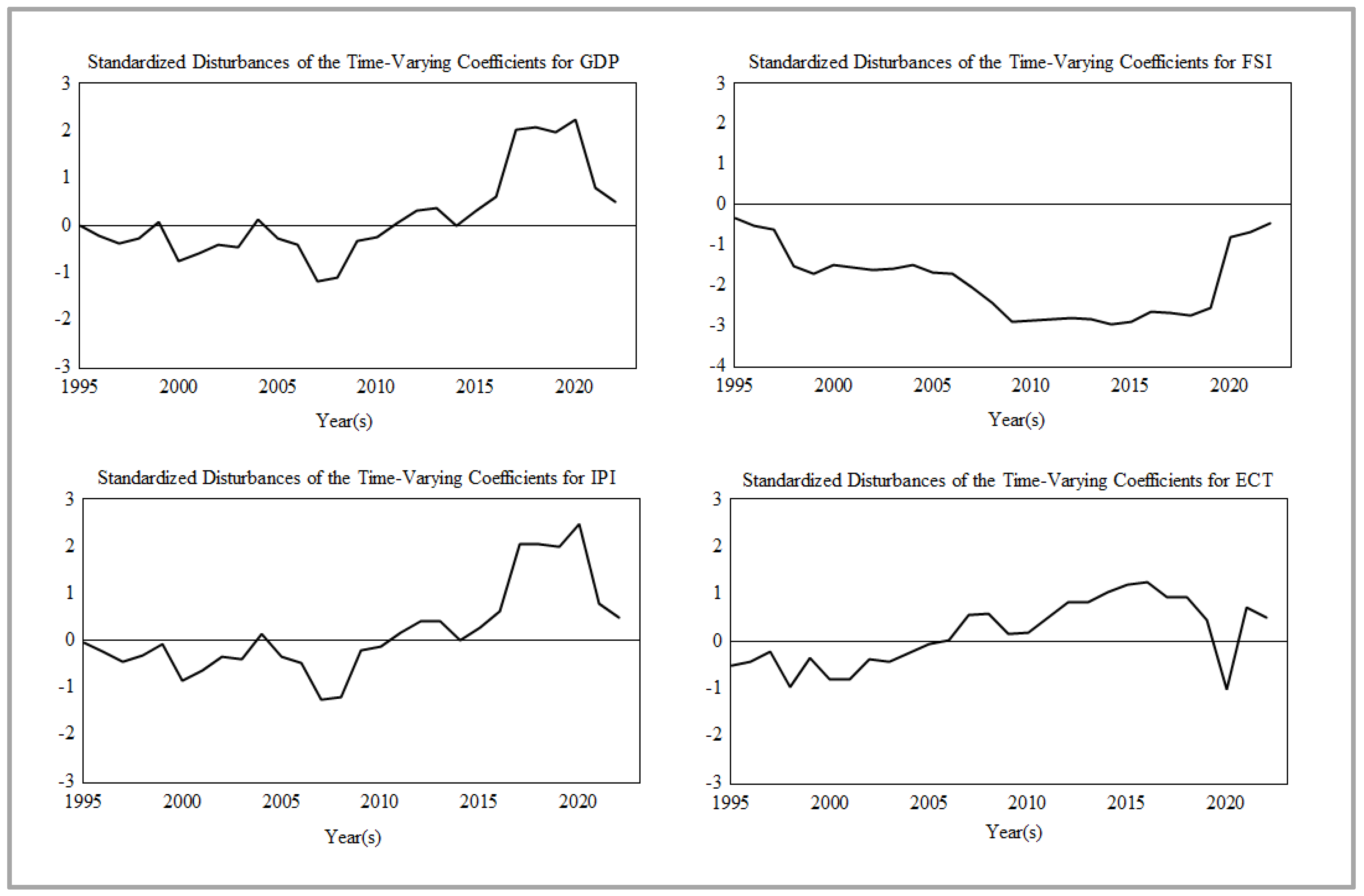
The time-varying coefficient estimates for FS, GDP, IP, and the ECT in Türkiye’s economy over the period of 1992–2021 are obtained using the Kalman filter and reported in

Table 6. Time-varying coefficient estimates.

Years	($\mathit{\gamma }$) FSI	($\mathit{\delta }$) GDP	($\mathit{\vartheta }$) IP	($\mathit{\lambda }$) ECT
1992	0.1676	0.1575	0.2207	−0.0454
1993	−0.2306	0.7816	0.7565	−0.3559
1994	−0.0388	0.3933	0.4166	−0.4235
1995	−0.3311	−0.0034	−0.0561	−0.5204
1996	−0.5234	−0.2170	−0.2464	−0.4426
1997	−0.6363	−0.3880	−0.4509	−0.2322
1998	−1.5204	−0.2750	−0.3183	−0.9644
1999	−1.7312	0.0610	−0.0737	−0.3509
2000	−1.4917	−0.7598	−0.8680	−0.8170
2001	−1.5742	−0.6048	−0.6446	−0.8242
2002	−1.6412	−0.4171	−0.3444	−0.3996
2003	−1.6086	−0.4658	−0.3958	−0.4459
2004	−1.5175	0.1083	0.1360	−0.2485
2005	−1.6897	−0.2697	−0.3495	−0.0680
2006	−1.7355	−0.4212	−0.4774	0.0050
2007	−2.0599	−1.1822	−1.2776	0.5387
2008	−2.4398	−1.1213	−1.2163	0.5812
2009	−2.9179	−0.3268	−0.2071	0.1460
2010	−2.8978	−0.2613	−0.1454	0.1821
2011	−2.8695	0.0532	0.1747	0.4830
2012	−2.8128	0.3178	0.4006	0.8081
2013	−2.8601	0.3637	0.4122	0.8108
2014	−2.9810	−0.0151	−0.0020	1.0194
2015	−2.9217	0.2967	0.2642	1.1786
2016	−2.6693	0.5905	0.6158	1.2392
2017	−2.7105	2.0132	2.0393	0.9307
2018	−2.7461	2.0662	2.0574	0.9248
2019	−2.5635	1.9807	1.9933	0.4442
2020	−0.8007	2.2438	2.4769	−1.0255
2021	−0.6926	0.7985	0.7718	0.7080

Source: author’s calculations.

(see Appendix A). The estimates indicate that FS is associated with a negative effect on EP throughout the 1990s, a period marked by increasing economic integration. During the 1997–2015 period, the magnitude of this negative association becomes more pronounced, coinciding with major economic disruptions, including the 2001 banking crisis and the 2008 global financial crisis. From 2016 onward, the estimated coefficients suggest a gradual weakening of the negative effect of FS on EP. Nevertheless, as of 2021, the estimated coefficients indicate that FS continues to have a negative effect on EP. Overall, the time-varying estimates indicate that the effect of FS on EP evolves over time and exhibits sensitivity to different phases of economic activity in Türkiye.

Secondly, turning to the time-varying effect of GDP on EP, the estimated coefficients indicate a positive effect during the 1992–1994 period. Between 1995 and 2010, however, the effect of GDP on EP is predominantly negative, with the exceptions of 1999 and 2004. Following the global financial crisis of 2008, the estimated effect changes sign again after 2010, with GDP exhibiting a positive effect on EP from 2014 onward. After 2020, the magnitude of this positive effect gradually diminishes in the aftermath of the COVID-19 pandemic. Taken together, the time-varying estimates suggest that the effect of GDP on EP varies over time.

Thirdly, with regard to the time-varying coefficients capturing the effect of the IP on EP, the estimates indicate a positive effect during the 1992–1994 period. Between 1995 and 2010, the estimated coefficients predominantly point to a negative effect of IP on EP. After 2010, with the exception of 2004, the estimates suggest that the effect of IP on EP becomes positive again, although its magnitude varies over time. Following the COVID-19 pandemic, the positive effect of IP on EP gradually weakens. Collectively, the time-varying estimates indicate that the effect of IP on EP differs across periods and changes in both sign and size over time.

Finally, an examination of the time-varying ECT coefficients reveals notable changes over the sample period. The estimated ECT coefficient remains negative between 1992 and 2005, indicating that deviations from the long-run equilibrium were gradually adjusted during this period. Between 2006 and 2015, however, the coefficient exhibits a weakening adjustment pattern, suggesting a reduced speed of convergence toward the long-run equilibrium. Toward the end of the 2000s, the upward movement of the ECT coefficient implies a decline in the strength of the adjustment mechanism. Although the estimates point to a partial improvement in the adjustment process around 2020, this pattern does not persist into 2021, indicating that the speed of adjustment remained limited in the final period of the sample.

5. Conclusions

The progress of countries toward sustainable development objectives is commonly assessed within the framework of ESG performance, of which environmental performance constitutes a central component. Environmental performance remains closely linked to countries’ development trajectories, particularly in the context of production expansion and resource use. For developing economies, balancing economic activity with environmental performance remains a key challenge, with Türkiye providing a relevant case for analysis. Motivated by that context, this study examines the effects of financial stability, economic growth, and industrial production on environmental performance in Türkiye using a Markov-switching error correction framework and time-varying parameter state–space model covering the period of 1990–2023.

The empirical findings from the Markov-switching ECM indicate that the effects of financial stability and economic growth on environmental performance are regime-dependent and differ across regimes. Specifically, financial stability is statistically insignificant in the low error-variance regime, whereas in the high error-variance regime, it exhibits a negative and statistically significant association with environmental performance. In contrast, economic growth displays a statistically significant negative association with environmental performance in the low-variance regime, while this association becomes statistically insignificant in the high-variance regime. These findings suggest that the relationships between financial stability, economic growth, and environmental performance vary across regimes. Moreover, industrial production exhibits a positive and statistically significant association with environmental performance in both regimes, although the magnitude of this association differs across regimes. Consistent with these regime-dependent findings, results from the time-varying parameter state–space model indicate that the effects of financial stability, economic growth, and industrial production on environmental performance also vary over time. During periods of heightened economic stress, the estimated coefficients are associated with lower environmental performance, while in subsequent periods, these effects weaken or change sign. In addition, the time-varying estimates of the error correction mechanism suggest that the speed of adjustment toward the long-run equilibrium is not constant over time.

The findings indicate that the impact of economic activity on environmental performance in Türkiye is neither constant across regimes nor stable over time, highlighting the importance of accounting for regime-dependent and time-varying dynamics in environmental assessments. The results further suggest that financial stability, economic growth, and industrial production do not exert homogeneous effects, implying that the environmental implications of economic activity should be evaluated within prevailing macro-financial conditions. This study provides additional evidence on the macro finance–environment nexus in Türkiye’s economy by employing a framework that incorporates regime-dependent structures and time-varying coefficients, offering an alternative to approaches based on average effect assumptions. Despite these contributions, the analysis remains subject to certain limitations, as it focuses exclusively on the environmental dimension of ESG performance and does not incorporate variables such as technological intensity, research and development activities, or foreign direct investment. Future studies may extend this framework by integrating these factors to enable a more comprehensive and multidimensional assessment.

References

1. Abbas, S., Ghosh, S., Sucharita, S., Dogan, B., Değer, O., & Mariev, O. (2025). Going green: Understanding the impacts of economic complexity, clean energy and natural resources on ecological footprint in complex economies. Environment, Development and Sustainability, 27(3), 6539–6565. [Google Scholar] [CrossRef] [Scilit]
2. Acheampong, A. O. (2019). Modelling for insight: Does financial development improve environmental quality? Energy Economics, 83, 156–179. [Google Scholar] [CrossRef] [Scilit]
3. Adebayo, T. S., Eweade, B. S., Özkan, O., & Uzun Ozsahin, D. (2025). Effects of energy security and financial development on load capacity factor in the USA: A wavelet kernel-based regularized least squares approach. Clean Technologies and Environmental Policy, 27, 4215–4232. [Google Scholar] [CrossRef] [Scilit]
4. Ali, M., Kirikkaleli, D., & Altuntaş, M. (2024). The nexus between CO2 intensity of GDP and environmental degradation in South European countries. Environment, Development and Sustainability, 26(5), 11089–11100. [Google Scholar] [CrossRef] [Scilit]
5. Antweiler, W., Copeland, B. R., & Taylor, M. S. (2001). Is free trade good for the environment? American Economic Review, 91(4), 877–908. [Google Scholar] [CrossRef] [Scilit]
6. Aybudak, H. G., Khalid, W., Usman, M., Seraj, M., Rafay, A., & Ali, Q. S. (2025). Assessing the impacts of economic growth, stringent environmental policies, renewable energy, and non-renewable energy on environmental sustainability in G-7 economies: Insights from the method of moments quantile regression. Asia-Pacific Journal of Regional Science, 9, 743–772. [Google Scholar] [CrossRef] [Scilit]
7. Azzone, G., Noci, G., Manzini, R., Welford, R., & Young, C. W. (1996). Defining environmental performance indicators: An integrated framework. Business Strategy and the Environment, 5(2), 69–80. [Google Scholar] [CrossRef] [Scilit]
8. Balcilar, M., Ozdemir, Z. A., & Shahbaz, M. (2019). On the time-varying links between oil and gold: New insights from the rolling and recursive rolling approaches. International Journal of Finance & Economics, 24(3), 1047–1065. [Google Scholar] [CrossRef] [Scilit]
9. Benkraiem, R., El-Khatib, Y., Fan, J., Goutte, S., & Klein, T. (2025). Optimal risk management considering environmental and climatic changes. Risk Analysis, 45(3), 544–562. [Google Scholar] [CrossRef] [Scilit]
10. Bentz, Y. (2003). Quantitative equity investment management with time-varying factor sensitivities. In Applied quantitative methods for trading and investment (pp. 213–237). John Wiley & Sons. [Google Scholar]
11. Berg, F., Kölbel, J. F., & Rigobon, R. (2022). Aggregate confusion: The divergence of ESG ratings. Review of Finance, 26(6), 1315–1344. [Google Scholar] [CrossRef] [Scilit]
12. Billingsley, P. (1961). Statistical methods in Markov chains. The Annals of Mathematical Statistics, 32(1), 12–40. [Google Scholar] [CrossRef] [Scilit]
13. Broto, C., & Ruiz, E. (2004). Estimation methods for stochastic volatility models: A survey. Journal of Economic Surveys, 18(5), 613–649. [Google Scholar] [CrossRef] [Scilit]
14. Burke, C. J., & Rosenblatt, M. (1958). A Markovian function of a Markov chain. The Annals of Mathematical Statistics, 29(4), 1112–1122. [Google Scholar] [CrossRef] [Scilit]
15. Chang, C. P., & Hao, Y. (2017). Environmental performance, corruption and economic growth: Global evidence using a new data set. Applied Economics, 49(5), 498–514. [Google Scholar] [CrossRef] [Scilit]
16. Chung, C. Y., Le, T. H., & Nguyen, T. H. V. (2025). Climate risk exposure and firm default risk: OECD insights into the moderating role of innovation. Asia-Pacific Journal of Financial Studies, 54(5), 570–596. [Google Scholar] [CrossRef] [Scilit]
17. Cole, M. A., & Elliott, R. J. (2005). FDI and the capital intensity of “dirty” sectors: A missing piece of the pollution haven puzzle. Review of Development Economics, 9(4), 530–548. [Google Scholar] [CrossRef] [Scilit]
18. Çabaş, M., Beşer, N. Ö., Ayaydın, H., Barut, A., & Magazzino, C. (2025). Greening the OECD: Unravelling the complex relationship between natural resource efficiency, technological innovation and population density on ecological footprint. Geological Journal, 60(11), 2621–2633. [Google Scholar] [CrossRef] [Scilit]
19. Dafermos, Y., Nikolaidi, M., & Galanis, G. (2018). Climate change, financial stability and monetary policy. Ecological Economics, 152, 219–234. [Google Scholar] [CrossRef] [Scilit]
20. Dar, J. A., & Asif, M. (2018). Does financial development improve environmental quality in Turkey? An application of endogenous structural breaks based cointegration approach. Management of Environmental Quality: An International Journal, 29(2), 368–384. [Google Scholar] [CrossRef] [Scilit]
21. Degirmenci, T., Acikgoz, F., Guney, E., & Aydin, M. (2025). Decoupling sustainable development from environmental degradation: Insights from environmental policy stringency, renewable energy, economic growth, and load capacity factor in high-income countries. Clean Technologies and Environmental Policy, 27(6), 2547–2563. [Google Scholar] [CrossRef] [Scilit]
22. Deschamps, P. J. (2008). Comparing smooth transition and Markov switching autoregressive models of US unemployment. Journal of Applied Econometrics, 23(4), 435–462. [Google Scholar] [CrossRef] [Scilit]
23. Destek, M. A., & Sarkodie, S. A. (2019). Investigation of environmental Kuznets curve for ecological footprint: The role of energy and financial development. Science of the Total Environment, 650, 2483–2489. [Google Scholar] [CrossRef] [Scilit] [PubMed]
24. Diaye, M. A., Ho, S. H., & Oueghlissi, R. (2022). ESG performance and economic growth: A panel co-integration analysis. Empirica, 49(1), 99–122. [Google Scholar] [CrossRef] [Scilit]
25. Dickey, D. A., & Fuller, W. A. (1979). Distribution of the estimators for autoregressive time series with a unit root. Journal of the American Statistical Association, 74(366a), 427–431. [Google Scholar] [CrossRef] [Scilit]
26. Donaldson, L. (2001). The contingency theory of organizations. Sage. [Google Scholar]
27. Dridi, D., Hasni, R., & Kahia, M. (2025). Environmental degradation and financial development nexus in BRICS plus countries: Do financial development drivers make a difference? Journal of the Knowledge Economy, 16(2), 10222–10254. [Google Scholar] [CrossRef] [Scilit]
28. Dueker, M. J., Psaradakis, Z., Sola, M., & Spagnolo, F. (2013). State-dependent threshold smooth transition autoregressive models. Oxford Bulletin of Economics and Statistics, 75(6), 835–854. [Google Scholar] [CrossRef] [Scilit]
29. Durbin, J., & Koopman, S. J. (2012). Time series analysis by state space methods. Oxford University Press. [Google Scholar]
30. Engle, R. F., & Granger, C. W. (1987). Co-integration and error correction: Representation, estimation, and testing. Econometrica: Journal of the Econometric Society, 55(2), 251–276. [Google Scholar] [CrossRef] [Scilit]
31. Erdogan, S., & Solarin, S. A. (2025). Does mineral-driven renewable energy production promote sustainable development? Uncovering the moderating role of economic development. Journal of Environmental Management, 391, 126598. [Google Scholar] [CrossRef] [Scilit]
32. Faizi, A., Ak, M. Z., Alsabhan, T. H., Shahzad, M. R., Alshagri, R., & Khan, S. (2025). Evaluating the role of renewable energy natural resources and globalization in environmental quality in OIC countries. Scientific Reports, 15(1), 33496. [Google Scholar] [CrossRef] [Scilit]
33. Frömmel, M., MacDonald, R., & Menkhoff, L. (2005). Markov switching regimes in a monetary exchange rate model. Economic Modelling, 22(3), 485–502. [Google Scholar] [CrossRef] [Scilit]
34. Frühwirth-Schnatter, S. (1995). Bayesian model discrimination and Bayes factors for linear Gaussian state space models. Journal of the Royal Statistical Society: Series B (Methodological), 57(1), 237–246. [Google Scholar] [CrossRef] [Scilit]
35. Gani, A. (2021). Fossil fuel energy and environmental performance in an extended STIRPAT model. Journal of Cleaner Production, 297, 126526. [Google Scholar] [CrossRef] [Scilit]
36. Ghani, M., & Qin, Q. (2025). Forecasting climate-sensitive industries’ volatility: A regime-switching GARCH-MIDAS approach with multiple climate risk indicators. International Review of Financial Analysis, 105, 104412. [Google Scholar] [CrossRef] [Scilit]
37. Grossman, G. M., & Krueger, A. B. (1995). Economic growth and the environment. The Quarterly Journal of Economics, 110(2), 353–377. [Google Scholar] [CrossRef] [Scilit]
38. Hamilton, J. D. (1989). A new approach to the economic analysis of nonstationary time series and the business cycle. Econometrica: Journal of the Econometric Society, 57(2), 357–384. [Google Scholar] [CrossRef] [Scilit]
39. Hamilton, J. D. (2020). Time series analysis. Princeton University Press. [Google Scholar]
40. Hoffmann, V. H., & Busch, T. (2008). Corporate carbon performance indicators: Carbon intensity, dependency, exposure, and risk. Journal of Industrial Ecology, 12(4), 505–520. [Google Scholar] [CrossRef] [Scilit]
41. Ilinitch, A. Y., Soderstrom, N. S., & Thomas, T. E. (1998). Measuring corporate environmental performance. Journal of Accounting and Public Policy, 17(4–5), 383–408. [Google Scholar] [CrossRef] [Scilit]
42. International Monetary Fund. (2025). International financial statistics. Available online: https://data.imf.org/IFS (accessed on 23 December 2025).
43. Iqbal, M. A., Shaheen, W. A., Shabir, S., Ullah, U., Ionel-Alin, I., Mihut, M. I., Raposo, A., & Han, H. (2025). Towards a green economy: Investigating the impact of sustainable finance, green technologies, and environmental policies on environmental degradation. Journal of Environmental Management, 374, 124047. [Google Scholar] [CrossRef] [Scilit] [PubMed]
44. Jalil, A., & Feridun, M. (2011). The impact of growth, energy and financial development on the environment in China: A cointegration analysis. Energy Economics, 33(2), 284–291. [Google Scholar] [CrossRef] [Scilit]
45. Javed, A., Usman, M., & Rapposelli, A. (2025). Transition toward a sustainable future: Exploring the role of green investment, environmental policy, and financial development in the context of load capacity factor in G-7 countries. Sustainable Development, 33(2), 1589–1609. [Google Scholar] [CrossRef] [Scilit]
46. Ji, X., Zhang, Y., Mirza, N., Umar, M., & Rizvi, S. K. A. (2021). The impact of carbon neutrality on the investment performance: Evidence from the equity mutual funds in BRICS. Journal of Environmental Management, 297, 113228. [Google Scholar] [CrossRef] [Scilit]
47. Johansen, S. (1991). Estimation and hypothesis testing of cointegration vectors in Gaussian vector autoregressive models. Econometrica: Journal of the Econometric Society, 59(6), 1551–1580. [Google Scholar] [CrossRef] [Scilit]
48. Kalman, R. E. (1960). A new approach to linear filtering and prediction problems. Journal of Basic Engineering, 82(1), 35–45. [Google Scholar] [CrossRef] [Scilit]
49. Kalman, R. E., & Bucy, R. S. (1961). New results in linear filtering and prediction theory. Journal of Basic Engineering, 83(1), 95–108. [Google Scholar] [CrossRef] [Scilit]
50. Kandepu, R., Foss, B., & Imsland, L. (2008). Applying the unscented Kalman filter for nonlinear state estimation. Journal of Process Control, 18(7–8), 753–768. [Google Scholar] [CrossRef] [Scilit]
51. Kapetanios, G., Shin, Y., & Snell, A. (2006). Testing for cointegration in nonlinear smooth transition error correction models. Econometric Theory, 22(2), 279–303. [Google Scholar] [CrossRef] [Scilit]
52. Kelly, A. M., & Nembot Ndeffo, L. (2025). Understanding the nexus: Economic complexity and environmental degradation in Sub-Saharan Africa. Clean Technologies and Environmental Policy, 27(1), 423–437. [Google Scholar] [CrossRef] [Scilit]
53. Khalid, W., Nawaz, A., Gadou, L. M. A., Khan, S. U., & Aybudak, H. G. (2025). Examining short-run and long-run nexus between economic growth, financial development, energy consumption and environmental degradation: Empirical evidence for the environmental Kuznets curve hypothesis in Egypt. Asia-Pacific Journal of Regional Science, 9, 479–511. [Google Scholar] [CrossRef] [Scilit]
54. Kihombo, S., Ahmed, Z., Chen, S., Adebayo, T. S., & Kirikkaleli, D. (2021). Linking financial development, economic growth, and ecological footprint: What is the role of technological innovation? Environmental Science and Pollution Research, 28(43), 61235–61245. [Google Scholar] [CrossRef] [Scilit] [PubMed]
55. Kim, Y. B., An, H. T., & Kim, J. D. (2015). The effect of carbon risk on the cost of equity capital. Journal of Cleaner Production, 93, 279–287. [Google Scholar] [CrossRef] [Scilit]
56. Krueger, P., Sautner, Z., & Starks, L. T. (2020). The importance of climate risks for institutional investors. The Review of Financial Studies, 33(3), 1067–1111. [Google Scholar] [CrossRef] [Scilit]
57. Lan, J., Kakinaka, M., & Huang, X. (2012). Foreign direct investment, human capital and environmental pollution in China. Environmental and Resource Economics, 51(2), 255–275. [Google Scholar] [CrossRef] [Scilit]
58. Landi, G. C., Iandolo, F., Renzi, A., & Rey, A. (2022). Embedding sustainability in risk management: The impact of environmental, social, and governance ratings on corporate financial risk. Corporate Social Responsibility and Environmental Management, 29(4), 1096–1107. [Google Scholar] [CrossRef] [Scilit]
59. Li, Z., Dong, H., Huang, Z., & Failler, P. (2019). Impact of foreign direct investment on environmental performance. Sustainability, 11(13), 3538. [Google Scholar] [CrossRef] [Scilit]
60. Ma, B., & Wang, A. (2025). Exploring the role of renewable energy in green job creation and sustainable economic development: An empirical approach. Energy Strategy Reviews, 58, 101642. [Google Scholar] [CrossRef] [Scilit]
61. Maitland-Smith, J. K., & Brooks, C. (1999). Threshold autoregressive and Markov switching models: An application to commercial real estate. Journal of Property Research, 16(1), 1–19. [Google Scholar] [CrossRef] [Scilit]
62. Meinhold, R. J., & Singpurwalla, N. D. (1983). Understanding the Kalman filter. The American Statistician, 37(2), 123–127. [Google Scholar] [CrossRef] [Scilit]
63. Owen, R., Brennan, G., & Lyon, F. (2018). Enabling investment for the transition to a low carbon economy: Government policy to finance early stage green innovation. Current Opinion in Environmental Sustainability, 31, 137–145. [Google Scholar] [CrossRef] [Scilit]
64. Ozcan, B., Apergis, N., & Shahbaz, M. (2018). A revisit of the environmental Kuznets curve hypothesis for Turkey: New evidence from bootstrap rolling window causality. Environmental Science and Pollution Research, 25(32), 32381–32394. [Google Scholar] [CrossRef] [Scilit]
65. Ozturk, I., & Acaravci, A. (2013). The long-run and causal analysis of energy, growth, openness and financial development on carbon emissions in Turkey. Energy Economics, 36, 262–267. [Google Scholar] [CrossRef] [Scilit]
66. Özsoy, T. (2024). The “energy rebound effect” within the framework of environmental sustainability. Wiley Interdisciplinary Reviews: Energy and Environment, 13(2), e517. [Google Scholar] [CrossRef] [Scilit]
67. Pata, U. K. (2018). Renewable energy consumption, urbanization, financial development, income and CO2 emissions in Turkey: Testing EKC hypothesis with structural breaks. Journal of Cleaner Production, 187, 770–779. [Google Scholar] [CrossRef] [Scilit]
68. Pesaran, M. H., & Timmermann, A. (2002). Market timing and return prediction under model instability. Journal of Empirical Finance, 9(5), 495–510. [Google Scholar] [CrossRef] [Scilit]
69. Phillips, P. C., & Perron, P. (1988). Testing for a unit root in time series regression. Biometrika, 75(2), 335–346. [Google Scholar] [CrossRef]
70. Psaradakis, Z., Sola, M., & Spagnolo, F. (2004). On Markov error-correction models, with an application to stock prices and dividends. Journal of Applied Econometrics, 19(1), 69–88. [Google Scholar] [CrossRef] [Scilit]
71. Rehman, A., Rauf, A., Ahmad, M., Chandio, A. A., & Deyuan, Z. (2019). The effect of carbon dioxide emission and the consumption of electrical energy, fossil fuel energy, and renewable energy, on economic performance: Evidence from Pakistan. Environmental Science and Pollution Research, 26(21), 21760–21773. [Google Scholar] [CrossRef] [Scilit]
72. Ren, S., Hao, Y., & Wu, H. (2022). How does green investment affect environmental pollution? Evidence from China. Environmental and Resource Economics, 81(1), 25–51. [Google Scholar] [CrossRef] [Scilit]
73. Rjoub, H., Odugbesan, J. A., Adebayo, T. S., & Wong, W. K. (2021). Sustainability of the moderating role of financial development in the determinants of environmental degradation: Evidence from Turkey. Sustainability, 13(4), 1844. [Google Scholar] [CrossRef] [Scilit]
74. Sadorsky, P. (2010). The impact of financial development on energy consumption in emerging economies. Energy Policy, 38(5), 2528–2535. [Google Scholar] [CrossRef] [Scilit]
75. Sadorsky, P. (2011). Financial development and energy consumption in Central and Eastern European frontier economies. Energy Policy, 39(2), 999–1006. [Google Scholar] [CrossRef] [Scilit]
76. Shahbaz, M., Hye, Q. M. A., Tiwari, A. K., & Leitão, N. C. (2013c). Economic growth, energy consumption, financial development, international trade and CO2 emissions in Indonesia. Renewable and Sustainable Energy Reviews, 25, 109–121. [Google Scholar] [CrossRef] [Scilit]
77. Shahbaz, M., Solarin, S. A., Mahmood, H., & Arouri, M. (2013a). Does financial development reduce CO2 emissions in Malaysian economy? A time series analysis. Economic Modelling, 35, 145–152. [Google Scholar] [CrossRef] [Scilit]
78. Shahbaz, M., Tiwari, A. K., & Nasir, M. (2013b). The effects of financial development, economic growth, coal consumption and trade openness on CO2 emissions in South Africa. Energy Policy, 61, 1452–1459. [Google Scholar] [CrossRef] [Scilit]
79. Shaheen, A., Sheng, J., Arshad, S., Muhammad, H., & Salam, S. (2025). Forecasting the determinants of environmental degradation: A gray modeling approach. Energy Sources, Part A: Recovery, Utilization, and Environmental Effects, 47(1), 1084–1104. [Google Scholar] [CrossRef] [Scilit]
80. Shahrour, M. H., Arouri, M., & Lemand, R. (2023). On the foundations of firm climate risk exposure. Review of Accounting and Finance, 22(5), 620–635. [Google Scholar] [CrossRef] [Scilit]
81. Sun, L., Fang, S., Iqbal, S., & Bilal, A. R. (2022). Financial stability role on climate risks, and climate change mitigation: Implications for green economic recovery. Environmental Science and Pollution Research, 29(22), 33063–33074. [Google Scholar] [CrossRef] [Scilit]
82. Swanson, N. R., & White, H. (1997). A model selection approach to real-time macroeconomic forecasting using linear models and artificial neural networks. Review of Economics and Statistics, 79(4), 540–550. [Google Scholar] [CrossRef] [Scilit]
83. Tamazian, A., & Rao, B. B. (2010). Do economic, financial and institutional developments matter for environmental degradation? Evidence from transitional economies. Energy Economics, 32(1), 137–145. [Google Scholar] [CrossRef] [Scilit]
84. Tunio, F. H., Nabi, A. A., Memon, R. U. R., Fraz, T. R., & Haluza, D. (2025). Sustainability in high-income countries: Urbanization, renewables, and ecological footprints. Energies, 18(7), 1599. [Google Scholar] [CrossRef] [Scilit]
85. Tutgun, S. (2025). Analysis of the interaction between ecological footprint, green technology and financial development in Türkiye: Evidence from fourier ARDL approach. Üçüncü Sektör Sosyal Ekonomi Dergisi, 60(2), 1459–1481. [Google Scholar] [CrossRef] [Scilit]
86. Uche, E., Das, N., Bera, P., & Cifuentes-Faura, J. (2023). Understanding the imperativeness of environmental-related technological innovations in the FDI–environmental performance nexus. Renewable Energy, 206, 285–294. [Google Scholar] [CrossRef] [Scilit]
87. United Nations Framework Convention on Climate Change. (2015). Paris agreement. Available online: https://unfccc.int/process-and-meetings/the-paris-agreement/the-paris-agreement (accessed on 23 December 2025).
88. Weber, O. (2017). Corporate sustainability and financial performance of Chinese banks. Sustainability Accounting, Management and Policy Journal, 8(3), 358–385. [Google Scholar] [CrossRef] [Scilit]
89. Wen, J., Mughal, N., Zhao, J., Shabbir, M. S., Niedbała, G., Jain, V., & Anwar, A. (2021). Does globalization matter for environmental degradation? Nexus among energy consumption, economic growth, and carbon dioxide emission. Energy Policy, 153, 112230. [Google Scholar] [CrossRef] [Scilit]
90. Woods, J. W. (2005). Two-dimensional Kalman filtering. In Two-dimensional digital signal processing I: Linear filters (pp. 155–205). Springer. [Google Scholar] [CrossRef] [Scilit]
91. World Bank. (2025a). Global financial development indicators. Available online: https://databank.worldbank.org/source/global-financial-development (accessed on 23 December 2025).
92. World Bank. (2025b). The world development indicators (WDI) database. Available online: https://databank.worldbank.org/source/world-development-indicators (accessed on 23 December 2025).
93. Wu, S., & Chen, R. (2007). Threshold variable determination and threshold variable driven switching autoregressive models. Statistica Sinica, 17(1), 241–264. [Google Scholar]
94. Wursthorn, S., Poganietz, W. R., & Schebek, L. (2011). Economic–environmental monitoring indicators for European countries: A disaggregated sector-based approach for monitoring eco-efficiency. Ecological Economics, 70(3), 487–496. [Google Scholar] [CrossRef] [Scilit]
95. Yardımcı, P., & Oskay, C. (2025). The impact of green finance and financial globalization on environmental sustainability: Empirical evidence from Türkiye. Sustainability, 17(13), 5696. [Google Scholar] [CrossRef] [Scilit]
96. Yurtkuran, S., & Güneysu, Y. (2023). Financial inclusion and environmental pollution in Türkiye: Fresh evidence from load capacity curve using AARDL method. Environmental Science and Pollution Research, 30(47), 104450–104463. [Google Scholar] [CrossRef] [Scilit] [PubMed]
97. Yurtkuran, S., & Güneysu, Y. (2026). The impact of green finance and financial technology on environmental pollution: Testing the LCC hypothesis for Türkiye. Journal of Environmental Management, 397, 128191. [Google Scholar] [CrossRef] [Scilit] [PubMed]
98. Zhang, Y. J. (2011). The impact of financial development on carbon emissions: An empirical analysis in China. Energy Policy, 39(4), 2197–2203. [Google Scholar] [CrossRef] [Scilit]
99. Zivot, E., & Wang, J. (2003). Rolling analysis of time series. In Modeling financial time series with S-Plus® (pp. 299–346). Springer. [Google Scholar] [CrossRef] [Scilit]