A Quantum Leap in Asset Pricing: Explaining Anomalous Returns

Abstract

This paper investigates the ability of asset pricing models to explain the cross-section of average stock returns of anomaly portfolios. A large sample of 286 anomaly portfolios are employed. We perform out-of-sample cross-sectional regression tests of both prominent asset pricing models and a relatively new model dubbed the ZCAPM. Empirical tests strongly support the lesser known ZCAPM but not other multifactor models. Further analyses of out-of-sample mispricing errors of the models reveal that the ZCAPM provides much more accurate pricing of anomaly portfolios than other models. We conclude that anomalies are anomalous to popular multifactor models but not the ZCAPM. By implication, the efficient market hypothesis is supported.

1. Introduction

In his Presidential Address to the American Finance Association, Cochrane (2011) observed that a “factor zoo” exists in the field of asset pricing due to the proliferation of stock market anomalies. In a series of papers, Fama and French (1992, 1993, 1996, 1998) showed that the now famous capital asset pricing model (CAPM) of Sharpe (1964), Lintner (1965), Mossin (1966), and Treynor (1961, 1962) failed to explain stock returns in general and size and value anomalies in particular. High (low) beta stocks did not have higher (lower) returns than other stocks. In its place, they proposed a three-factor model that augmented the market factor with size and value factors. This innovative multifactor model did a good job of explaining the size and value anomalies.

Subsequently, consistent with Cochrane, researchers discovered hundreds of anomalies, which has evolved into two branches of literature. One branch documents the anomalies and tests for their persistence over time. The work by McLean and Pontiff (2016) investigated 97 anomaly portfolios and found that anomalies tended to diminish or disappear over time after their publication in academic journals. This diminution of anomalies has been confirmed by other researchers.1 By contrast, Jacobs and Muller (2020) examined 241 anomalies in 39 stock markets that (with the exception of the United States) did not tend to diminish in post-publication years. Another study by A. Y. Chen and Zimmermann (2020) found that prior publication only explains 12 percent of anomaly returns. Also, Jensen et al. (2023) found that 153 long/short factors across 93 countries can be replicated over time, hold on an out-of-sample basis after their original publication, are supported by the large number of factors including global evidence, and can be combined into a smaller number of anomaly clusters. Unlike previous studies, the authors used alphas from the CAPM to measure anomaly returns. They found that risk-adjusted returns yield different results than raw returns. Another recent paper by Bowles et al. (2023) explored the timing of anomalies and found that anomaly returns persist but decay rapidly after information release dates. Previous studies that rebalance anomaly portfolios on an annual basis (for example) incorporate stale information. In their study, using real-time data after information events, anomaly returns did not decrease over time. Hence, they concluded that event-based anomalies were alive and well in financial markets. Consistent with these studies, numerous authors ascribe to the notion that anomalies are real mispricing as opposed to data mining.2

A second branch of studies has sought to address the factor zoo problem by developing parsimonious asset pricing models that can explain many anomalies. For example, to explain 80 anomaly portfolios, Hou et al. (2015) proposed a four-factor model with market, size, profit, and capital investment factors.3 Also, using the same 80 anomaly portfolios, Stambaugh and Yuan (2017) specified a four-factor model with market, size, management, and performance factors that outperformed the Hou et al. (2015) model in terms of explanatory power. Thus, these studies suggest that low-dimension asset pricing models can be used to capture many anomalies.

We extend asset pricing studies by comparing the ability of multifactor models to explain large numbers of anomaly portfolio returns. Surprisingly, standard Fama and MacBeth (1973) cross-sectional regression tests show that a lesser known two-factor model dubbed the ZCAPM by Kolari et al. (2021) well outperforms prominent multifactor models in terms of explaining anomaly returns on an out-of-sample basis. In empirical tests, we utilize online databases of anomalies recently made available by researchers. A. Y. Chen and Zimmermann (2022) have provided an open source database with 161 long/short anomalies in the U.S. stock market.4 Also, Jensen et al. (2023) have furnished an online database containing 153 long/short anomalies in 93 countries including the U.S. Based on 133 (153) anomalies in the former (latter) study with return series available from 3 July 1972 to 31 December 2021, we investigate a combined dataset of 286 anomalies.

We find that, with the exception of the ZCAPM, prominent multifactor models do not explain anomaly portfolio returns. By contrast, the ZCAPM does a much better job of explaining them. In standard Fama and MacBeth (1973) cross-sectional regression tests, factor loadings for the ZCAPM are more significant than well-known multifactor models. Also, goodness-of-fit as estimated by $R^2$ values are much higher for the ZCAPM than other models. Further graphical tests compare the mispricing errors of different models with respect to anomaly portfolios. We find that the ZCAPM exhibits much lower mispricing errors than other models. We conclude that anomaly returns are anomalous for the most part with respect to prominent multifactor models but not the ZCAPM. By implication, our evidence supports the efficient market hypothesis of Fama (1970, 2013) rather than the behavioral hypothesis.5 As such, stock returns are closely related to systematic market risks.

The next section reviews the relevant literature. Section 3 describes the methodology. Section 4 reports and discusses the empirical evidence. The last section concludes.

2. Literature Review

The asset pricing literature has evolved over time to produce a wide variety of models to help explain stock market anomalies. Fama and French (1992, 1993) proposed the now famous three-factor model that augmented the market factor with size and value factors. The latter factors were shown to better explain portfolios of stocks sorted on size and value firm characteristics than the CAPM market factor alone. Carhart (1997) added a momentum factor to explain the momentum anomaly. Extending these multifactor models, Fama and French (2015) added profitability and capital investment factors. They found that the value factor could be dropped with similar ability of the resultant four-factor model to explain various anomaly portfolio sorted on size, value, profitability, and capital investment firm characteristics.

Expanding the study of anomalies, Hou et al. (2015) developed a four-factor model (with factors similar to those in the Fama and French four-factor model). They found that their model outperformed other models in terms of explaining the returns of 80 long/short anomaly portfolios. Like Fama and French, they utilized the in-sample Gibbons et al. (1989) (GRS) test for the joint equality of anomaly portfolios’ alpha estimates. Unlike the present study, they did not report out-of-sample cross-sectional regression test results. Another related study by Stambaugh and Yuan (2017) proposed a four-factor model including market, size, management, and performance factors. Using the same 80 anomaly portfolio as Hou et al., their model outperformed other models in GRS tests of model alphas.

Departing from long/short factors constructed by researchers, Lettau and Pelger (2020) tested a five-factor model based on latent (hidden) factors identified by principal component analysis (PCA). GRS tests showed that their model had lower mispricing errors (as measured by alphas for 370 portfolios sorted on various firm characteristics) than the Fama and French three- and five-factor models. In efforts to improve their model, Fama and French (2018) incorporated a momentum factor to form a six-factor model. This model appeared to perform well in alpha tests relative to their prior multifactor models.

Lastly, Kolari et al. (2021) proposed in a book a new asset pricing model dubbed the ZCAPM, mathematically derived as a special case of Black’s (1972) zero-beta CAPM. As reviewed in the next section, the ZCAPM has two factors: (1) beta risk related to average market returns and (2) zeta risk associated with cross-section market return dispersion. Empirical tests using size and value portfolios employed by Fama and French showed that the ZCAPM consistently outperformed their three-factor model in out-of-sample cross-sectional regression tests, at times by large margins. Additionally, lower average mispricing errors were documented for the ZCAPM than other multifactor models. Further tests of industry portfolios and individual stocks, as well as other anomaly portfolios sorted on firm characteristics, supported the ZCAPM, which outperformed a number of popular multifactor models.

Kolari et al. (2022) tested the ZCAPM using U.S. stocks for a long sample period from 1927 to 2020. The results confirmed the findings of Kolari et al. (2021). Again, in out-of-sample cross-sectional regression tests, the ZCAPM well outperformed the CAPM, Fama and French three-factor model, and Carhart four-factor model. Subperiod results by splitting sample observations continued to support the ZCAPM over the other models. As before, t-statistics corresponding to the market price of zeta risk related to market return dispersion loadings exceeded 3 that were higher than other factor loading market prices of risk. The authors concluded that the ZCAPM offers a parsimonious empirical model with only two factors and theoretical foundations in the general equilibrium CAPM and zero-beta CAPM asset pricing models.

Kolari et al. (2022) conducted tests of the ZCAPM on anomaly portfolios in Canada, France, Germany, Japan, the United Kingdom, and the United States. They compared the ZCAPM to the Fama and French three-factor model and Carhart four-factor model. In all countries, the ZCAPM outperformed these models in out-of-sample cross-sectional regression tests with higher $R^2$ values and t-statistics for zeta risk loadings. Also, average mispricing errors were substantially lower for the ZCAPM relative to the other models. They concluded that the ZCAPM is not a false discovery, which renews interest in the CAPM as a viable approach to asset pricing.

Recently, Kolari et al. (2024) applied the ZCAPM to constructing high return stock portfolios. The CRSP index exhibited much lower Sharpe ratios than these portfolios. Based on their evidence for U.S. stocks, the authors showed that the mean-variance investment parabola of Markowitz (1952, 1959) has an architecture that can be mapped in terms of the beta risk and zeta risk of portfolios. The CRSP index and S&P 500 index were located in the middle of their empirical depiction of the mean-variance investment parabola. All portfolios’ returns were computed out-of-sample in the month ahead of the estimation of risk parameters in the ZCAPM. Application of the ZCAPM to actively managed equity mutual funds showed that the ZCAPM could be used to help guide mutual fund investments by pension funds and other investors. We interpret their finding to suggest that more efficient portfolios with higher Sharpe ratios can be constructed using the ZCAPM to estimate beta risk and zeta risk measures.

3. Methodology

We download daily anomaly portfolio returns from the internet websites of A. Y. Chen and Zimmermann (2022) and Jensen et al. (2023). Of 161 clear predictor portfolios in the former dataset, 133 anomaly portfolios are retained with available returns from 3 July 1972 to 31 December 2021.6 The latter dataset includes 153 anomaly portfolios with available returns in this sample period. Appendix A and Appendix B contain lists of anomalies in these two respective databases. Factors for the models under study (to be discussed shortly) are downloaded from Kenneth French’s online database.7

3.1. Cross-Sectional Regression Tests

As already mentioned, we employ standard Fama and MacBeth (1973) tests. First, each model is estimated using a time-series regression. Second, risk loadings of factors in each model are used as independent variables in an out-of-sample (one-month-ahead) cross-sectional regression, which provides estimates of the market price of risk for loadings. More specifically, we begin by estimating the following time-series regression for the ith anomaly portfolio in the one-year estimation window from July 1972 to June 1973:

$$\begin{array}{c}\hfill R_{it}-R_{ft}={\alpha }_i+\sum _{k=1}^K{b}_{ik}{F}_{kt}+e_{it},t=1,\dots ,T,\end{array}$$

(1)

where $R_{it}-R_{ft}$ is the realized excess return on the ith test asset for day t; $R_{ft}$ is the riskless rate proxied by the Treasury bill rate; ${\alpha }_i$ is the intercept term or alpha; $F_{kt}$ are asset pricing factors for $k=1,\dots ,K$ factors; $b_{ik}$ are corresponding K beta risk loadings for the ith portfolio; $i=1,\dots ,N$ correspond to the number of portfolios; $t=1,\dots ,T$ is the estimation period; and $e_{it}\sim$ iid (0, ${\sigma }_i^2$).

Next, we estimate following out-of-sample cross-sectional regression in the next month of July 1973:

$$\begin{array}{c}\hfill R_{iT+1}-R_{fT+1}=\widehat{\alpha }+{\lambda }_1{\widehat{b}}_{i1}+{\lambda }_2{\widehat{b}}_{i2}+\dots +{\lambda }_K{\widehat{b}}_{iK}+u_{iT+1},i=1,\dots ,N,\end{array}$$

(2)

where $R_{iT+1}-R_{fT+1}$ is the realized excess return on the ith portfolio in out-of-sample (one-month-ahead) month $T+1$; $\widehat{\alpha }$ is the intercept; ${\widehat{b}}_{ik},k=1,\dots ,K$ are K beta risk loadings estimated for N anomaly portfolios in the estimation period $t=1,\dots ,T$; ${\lambda }_k$ are corresponding estimated market prices of beta risk loadings;8 and $u_{iT+1}$ are zero mean and independent of the explanatory variables.

The above two-step process is rolled forward one month at a time and repeated to generate a monthly time-series of market prices of risk, or ${\lambda }_k$ from July 1973 to December 2021. Subsequently, average market prices of risks and associated t-statistics are computed. Additionally, a monthly time series of realized and predicted returns for each portfolio from July 1973 to December 2021 is produced. Using these series, we compute average realized and average predicted returns for each of the 286 anomaly portfolios. Following Jagannathan and Wang (1996) and Lettau and Ludvigson (2001), a simple cross-sectional regression of average realized returns on average predicted returns is run to yield an estimate of the $R^2$ value. Lastly, we plot average realized returns against predicted returns to graphically illustrate mispricing errors for anomaly portfolios.

3.2. Asset Pricing Models

3.2.1. Prominent Asset Pricing Models

The following leading or renowned asset pricing models are studied:

• CAPM based on the market factor computed using the University of Chicago’s Center for Research in Security Prices (CRSP) value-weighted index minus the Treasury bill rate (M);
• Fama and French (1992, 1993)’s three-factor model (FF3) that augments the market factor with a size factor (small minus large firms’ stock returns, or SMB) and a value factor (high book-to-market equity minus low book-to-market equity firms’ stock returns, or HML);
• Carhart (1997)’s four-factor model (C4) that augments the three-factor model with a momentum factor (firms with high past return stock returns minus low past stock returns, or MOM);
• Fama and French (2015)’s five-factor model (FF5) that augments the three-factor model with a profit factor (robust operating profitability minus weak operating profitability returns, RMW) and capital investment factor (conservative investment minus aggressive investment returns, or CMA);
• Fama and French (2018)’s six-factor model (FF6) that augments the five-factor model with a momentum factor;

Additionally, we include the Kolari et al. (2021) ZCAPM that augments the market factor with a cross-sectional market return dispersion factor. Since many readers may be unfamiliar with the ZCAPM, we next provide an overview of this general equilibrium model.

3.2.2. Overview of ZCAPM

Kolari et al. (2021) (hereafter KLH) recently published a book that proposed a new asset pricing model dubbed the ZCAPM.9 Their model is mathematically derived as a special case of the now famous zero-beta CAPM by Black (1972). Two systematic risk factors emerge from their derivation: (1) average market return in excess of the riskless rate (i.e., market factor); and (2) cross-sectional standard deviation of returns in the market (i.e., market return dispersion). These factors are computed as the first and second moments of stock market returns on any given day. Note that the market dispersion factor is a cross-sectional rather than time-series standard deviation of returns.10 Market return dispersion is computed using the value-weighted CRSP index return (denoted $R_{at}$) on each day t as follows:

$${\sigma }_{at}=\sqrt{{\displaystyle \frac{n}{n-1}\sum _{i=1}^n{w}_{it-1}{(R_{it}-R_{at})}^2}},$$

(3)

where n is the total number of stocks; $w_{it-1}$ is the previous day’s market value weight for the ith stock (i.e., market capitalization of the stock divided by the market capitalization of all n stocks); $R_{it}$ is the return of the ith stock on day t; and $R_{at}$ is value-weighted average return of all available stocks in the CRSP database on day t. Many authors associate market return dispersion with macroeconomic shocks, such as economic uncertainty, business cycles, market volatility, and unemployment rates.11

The theoretical ZCAPM is closely related to the now famous mean-variance investment parabola of Markowitz (1952, 1959). KLH proved that the width or span of the parabola is determined by market return dispersion. Figure 1 shows the parabola with total risk (as measured by the time-series standard deviation of returns) on the X-axis and expected returns on the Y-axis. Interestingly, assuming the width is defined by market return dispersion, it must be true that the average market return lies somewhere along the axis of symmetry that divides the parabola into two symmetric halves. Thus, KLH inferred that the value-weighted CRSP index lies in the middle of the parabola, which is far from the efficient frontier. Many researchers have conjectured that the CRSP index represents an efficient portfolio and, therefore, is a plausible proxy for the market portfolio in the CAPM of Sharpe (1964). According to the ZCAPM, to reach the efficient frontier, investors should use the average market return to move along the axis of symmetry and then positive market return dispersion to move upward to the efficient frontier. Conversely, to reach the lower inefficient boundary of the parabola, investors can move downward from the axis of symmetry via negative market return dispersion. Importantly, market return dispersion can be positive or negative in sign for assets within the opportunity set described by the parabola.

In Figure 1, KLH chose two portfolios with the same time-series return variance (denoted ${\sigma }_P^2$) to derive the ZCAPM— namely, efficient portfolio $I^{\ast }$ and orthogonal inefficient zero-beta portfolio $Z{I}^{\ast }$. Simplifying their derivation, the expected returns of these two portfolios can be specified as follows:12

$$\begin{array}{ccc}\hfill E\left(R_{I^{\ast }}\right)& \approx & E\left(R_a\right)+{\sigma }_a\hfill \end{array}$$

(4)

$$\begin{array}{ccc}\hfill E\left(R_{Z{I}^{\ast }}\right)& \approx & E\left(R_a\right)-{\sigma }_a,\hfill \end{array}$$

(5)

where $E\left(R_a\right)$ is the average market return; and ${\sigma }_a$ is the market return dispersion.

Sharpe’s CAPM assumed perfect capital markets, homogeneous investor expectations, two-parameter probability distributions of returns, investor risk aversion, no short selling, and a riskless rate. Black amended the last two assumptions to allow short selling and borrowing at a rate greater than the riskless rate. His now famous zero-beta CAPM can be written as follows:

$$\begin{array}{ccc}\hfill E\left(R_i\right)& =& E\left(R_{ZM}\right)+{\beta }_{iM}[E\left(R_M\right)-E\left(R_{ZM}\right)],\hfill \end{array}$$

(6)

where $E\left(R_M\right)$ is the expected market portfolio return; $E\left(R_{ZM}\right)$ is the expected zero-beta portfolio return that is uncorrelated (orthogonal) to the market portfolio; and ${\beta }_{iM}$ is beta risk associated with excess expected market returns. According to Copeland and Weston (1980) and others, Black’s model can be more generally specified in terms of any efficient portfolio and its orthogonal inefficient portfolio:

$$\begin{array}{ccc}\hfill E\left(R_i\right)& =& E\left(R_{ZI}\right)+{\beta }_{iI}[E\left(R_I\right)-E\left(R_{ZI}\right)],\hfill \end{array}$$

(7)

where I and $ZI$ are any efficient index and its orthogonal zero-beta counterpart, respectively, located on the minimum variance boundary of the parabola.

Substituting the expected returns defined in Equations (4) and (5) into zero-beta CAPM relation (7), the theoretical ZCAPM is

$$\begin{array}{ccc}\hfill E\left(R_i\right)& =& E\left(R_{Z{I}^{\ast }}\right)+{\beta }_{i{I}^{\ast }}[E\left(R_{I^{\ast }}\right)-E\left(R_{Z{I}^{\ast }}\right)]\hfill \\ & =& E\left(R_a\right)-{\sigma }_a+{\beta }_{i{I}^{\ast }}\{[E\left(R_a\right)+{\sigma }_a]-[E\left(R_a\right)-{\sigma }_a]\}\hfill \\ & =& E\left(R_a\right)+(2{\beta }_{i{I}^{\ast }}-1){\sigma }_a\hfill \\ \hfill E\left(R_i\right)& =& E\left(R_a\right)+Z_{ia}^{\ast }{\sigma }_a,\hfill \end{array}$$

(8)

where $Z_{ia}^{\ast }=2{\beta }_{i{I}^{\ast }}-1$ (i.e., the systematic risk of asset i associated with ${\sigma }_a$). Notice that the theoretical ZCAPM is an alternative equivalent form of the zero-beta CAPM with respect to portfolios $I^{\ast }$ and $Z{I}^{\ast }$. Lastly, assuming the existence of a riskless rate asset, the theoretical ZCAPM can be respecified as follows:13

$$\begin{array}{c}\hfill E\left(R_i\right)-R_f={\beta }_{ia}[E\left(R_a\right)-R_f]+Z_{ia}^{\ast }{\sigma }_a,\end{array}$$

(10)

where ${\beta }_{ia}$ captures beta risk related to expected market excess returns; and $Z_{ia}^{\ast }$ is zeta risk associated with cross-sectional market return dispersion of expected returns of all assets in the market. As noted above, zeta risk can be positive or negative in sign with respect to the expected returns of portfolios $I^{\ast }$ and $Z{I}^{\ast }$, respectively.

In the ZCAPM, as the width of the parabola increases or decreases due to ${\sigma }_a$, the expected returns of assets within the parabola are affected. As ${\sigma }_a$ increases (decreases), assets in the upper half of the parabola above the axis of symmetry experience increasing (decreasing) expected returns; alternatively, assets in the bottom half of the parabola below the axis of symmetry experience decreasing (increasing) expected returns. It is obvious that market return dispersion has major impacts of the expected returns of assets in the market. Also, depending where assets are located within the parabola, these dispersion impacts can be positive or negative.

A major challenge for the ZCAPM is the specification of an empirical model that can capture both positive and negative market dispersion effects on assets’ returns. KLH proposed an innovative solution to this problem by introducing a hidden signal variable to model these two-sided dispersion effects at any given time t:

$$\begin{array}{c}\hfill R_{it}-R_{ft}={\alpha }_i+{\beta }_{ia}(R_{at}-R_{ft})+Z_{ia}{D}_{it}{\sigma }_{at}+u_{it},t=1,\dots ,T,\end{array}$$

(11)

where $Z_{ia}$ measures systematic risk associated with market return dispersion ${\sigma }_{at}$; $D_{it}$ is a hidden signal variable.14 $D_{it}$ is assigned values $+1$ and $-1$ to coincide with positive and negative market return dispersion effects on asset returns at time t, respectively; ${\alpha }_i$ is the intercept related to mispricing errors; $u_{it}\sim \mathrm{iid}\mathrm{N}(0,{\sigma }_i^2)$; and other notation is as before. In forthcoming analyses, we proxy average market returns, or $R_a$, with the value-weighted CRSP index return. Also, we proxy the market return dispersion using all common stocks in the CRSP database per Equation (3).

Unlike virtually all asset pricing models that employ ordinary least squares (OLS) regression, the empirical ZCAPM is estimated by means of the expectation-maximization (EM) algorithm, which is well known in the hard sciences.15 EM provides an estimate of the probability that hidden signal variable $D_{it}$ is $+1$ (p) or $-1$ ($1-p)$.16 In empirical ZCAPM regression relation (11), $D_{it}$ is an independent random variable with a two-point distribution:

$$\begin{array}{c}\hfill D_{it}=\left\{\begin{array}{cc}+1\hfill & \mathrm{with}\mathrm{probability}{p}_i\hfill \\ -1\hfill & \mathrm{with}\mathrm{probability}1-p_i,\hfill \end{array}\right.\end{array}$$

(12)

where $p_i$ (or $1-p_i$) is the probability of a positive (or negative) market return dispersion effect; and $D_{it}$ are independent of $u_{it}$. The EM algorithm estimates probability $p_i$ using available in-sample information about the dependent and independent variables in the model.

Based on Equation (11), $Z_{ia}{D}_{it}$ can take on values of $+Z_{ia}$ or $-Z_{ia}$ due to the sign of $D_{it}$. Since the mean of binary signal variable $D_{i,t}$ equals $2p_i-1$, we can define $Z_{ia}^{\ast }=Z_{ia}(2p_i-1)$. The parameter $Z_{ia}^{\ast }$ captures the systematic risk related to market return dispersion ${\sigma }_{at}$. Hence, the empirical ZCAPM can be written as follows:

$$\begin{array}{c}\hfill R_{it}-R_{ft}={\alpha }_i+{\beta }_{ia}(R_{at}-R_{ft})+Z_{ia}^{\ast }{\sigma }_{at}+u_{it},t=1,\dots ,T,\end{array}$$

(13)

where ${\beta }_{ia}$ and $Z_{ia}^{\ast }$ proxy beta risk and zeta risk parameters in the theoretical ZCAPM. In sample period $t=1,\dots ,T$, the sign of $Z_{ia}^{\ast }$ is based on the estimated probability $p_i$ of hidden variable $D_{it}$. Hence, if $p_i>1/2$ (or <1/2), the sign of $Z_{ia}^{\ast }$ is positive (negative). The empirical ZCAPM as estimated via EM is a probabilistic mixture model with two components, wherein one component has positive zeta risk and the other component has negative zeta risk.

We should mention that some authors have augmented the market factor with a market return dispersion factor, including Jiang (2010), Demirer and Jategaonkar (2013), and Garcia et al. (2014). Using OLS regression to estimate the time-series regression model and subsequent cross-sectional regression tests of factor loadings, they found both positive and negative sensitivity of stock returns to market return dispersion factor loadings. Sometimes, the latter factor loadings associated with market return dispersion were significant but not in other tests. We have found in repeated tests of the ZCAPM using many different test assets and sample time periods that zeta risk loadings are always significant in cross-sectional regression tests at high statistical levels that well exceed previous studies.

Unlike OLS regression asset pricing models, KLH found that the intercept parameter (or alpha) can be dropped from the empirical ZCAPM. No decrease in residual error variance was achieved by adding an intercept. For interested readers, KLH provide open source empirical ZCAPM software using Matlab, R, and Python programs on the internet at GitHub (https://github.com/zcapm, accessed on 1 January 2020). Programs for running Fama-MacBeth cross-sectional regression tests are available at this website also.

Finally, ZCAPM factor loadings for ${\widehat{\beta }}_{ia}$ and ${\widehat{Z}}_{ia}^{\ast }$ based on one year of daily returns prior to month $T+1$ are used to estimate the following OLS cross-sectional regression:

$$\begin{array}{c}\hfill R_{i,T+1}-R_{fT+1}={\lambda }_0+{\lambda }_a{\widehat{\beta }}_{ia}+{\lambda }_{RD}{\widehat{Z}}_{ia}^{\ast }+u_{it},i=1,\dots .,N,\end{array}$$

(14)

where ${\lambda }_0$ is the intercept term, ${\lambda }_a$ and ${\lambda }_{RD}$ are estimates of the market prices of beta risk and zeta risk loadings in percent terms, respectively, and the other notation is as before. It is notable that the dependent variable in this regression is the one-month ahead excess returns for the ith anomaly portfolio. Since zeta risk loadings are estimated using daily returns, we rescale the estimated zeta risk coefficient ${\widehat{Z}}_{i,a}^{\ast }$ from a daily to monthly basis as follows:

$$\begin{array}{c}\hfill R_{i,T+1}-R_{fT+1}={\lambda }_0+{\lambda }_M{\widehat{\beta }}_{ia}+{\lambda }_{RD}{\widehat{Z}}_{ia}^{\ast }{N}_{T+1}++u_{it},i=1,\dots .,N,\end{array}$$

(15)

where $N_{T+1}$ is the number of trading days in month $T+1$ (i.e., 21 days), $Z_{i,a}^{\ast }{N}_{T+1}$ is the monthly estimated zeta risk, and ${\lambda }_{RD}$ is the monthly risk premium associated with zeta risk. This rescaling does not change the risk premium ${\widehat{\lambda }}_{RD}$ in terms of each unit of zeta risk. Now, the estimated monthly market price of $Z_{i,a}^{\ast }$, or ${\lambda }_{RD}$, can be compared to the estimated monthly market price of ${\beta }_{ia}$, or ${\lambda }_a$.

4. Empirical Evidence

In this section, we report the results of cross-sectional regression tests of asset pricing models as well as comparative graphs of their average mispricing errors.

Table 1. Descriptive statistics for asset pricing factors. This table summarizes the descriptive statistics for the asset pricing factors. Distribution information is provided, including the mean return, standard deviation of returns, maximum and minimum returns, and 25th percentile (P25), median (P50), and 75th percentile (P75) returns. Daily factor returns (in percent) corresponding to different asset pricing models, are denoted as follows: ${\mathit{R}}_m-{\mathit{R}}_f$ (CRSP index return minus Treasury bill rate¹), $\mathit{SMB}$ (size), $\mathit{HML}$ (value), $\mathit{MOM}$ (momentum), $\mathit{RMW}$ (profit), $\mathit{CMA}$ (capital investment), and $\mathit{RD}$ (market return dispersion). The sample period is from July 1972 to December 2021.

Statistic	${\mathit{R}}_{\mathit{m}}-{\mathit{R}}_{\mathit{f}}$	$\mathit{SMB}$	$\mathit{HML}$	$\mathit{MOM}$	$\mathit{RMW}$	$\mathit{CMA}$	$\mathit{RD}$
Mean	0.01	0.005	0.01	0.03	0.01	0.01	1.86
Standard deviation	1.07	0.57	0.59	0.79	0.41	0.37	0.66
Maximum	11.35	6.17	6.74	7.12	4.52	2.53	10.77
Minimum	−17.47	−11.19	−5.00	−14.37	−3.01	−5.87	0.68
P25	−0.46	−0.30	−0.24	−0.25	−0.17	−0.18	1.47
P50	0.04	0.02	0.01	0.06	0.01	0.01	1.73
P75	0.53	0.32	0.26	0.36	0.19	0.19	2.04

¹ In the ZCAPM, due to using average market excess returns rather than a proxy for market portfolio excess returns, the market factor associated with CRSP index excess returns is denoted $R_a-R_f$ instead of $R_m-R_f$ per other models.

reports descriptive statistics for asset pricing factors in different models in our sample period. The market return dispersion factor ${\sigma }_{at}$ computed using Equation (3) is denoted as RD.

4.1. Cross-Sectional Regression Results

Table 2. Out-of-sample Fama–MacBeth cross-sectional tests of 286 anomaly portfolios for asset pricing models in the sample period July 1972 to December 2021. Using a total of 286 anomaly portfolios (comprising 133 plus 153 anomalous portfolios from A. Y. Chen and Zimmermann (2022) and Jensen et al. (2023), respectively), this table contains results for the sample period July 1972 to December 2021. Based on standard two-step Fama–MacBeth cross-sectional tests, we report out-of-sample (one-month-ahead) estimated market prices of risk denoted ${\widehat{\lambda }}_k$ for the kth factor for the analysis period July 1973 to December 2021. Associated t-statistics are shown in parentheses below estimated prices of risk. The asset pricing models are CAPM, Fama and French three-factor model (FF3), Carhart four-factor model (C4), Fama and French five-factor model (FF5), Fama and French six-factor model (FF6), and ZCAPM. Factors in these models are denoted as m (CRSP index excess return¹), $\mathit{RD}$ (market return dispersion), $\mathit{SMB}$ (size), $\mathit{HML}$ (value), $\mathit{MOM}$ (momentum), $\mathit{RMW}$ (profit), and $\mathit{CMA}$ (capital investment). The results are shown for the analysis period.

Model	$\widehat{\mathit{\alpha }}$	${\widehat{\mathit{\lambda }}}_{\mathit{m}}$	${\widehat{\mathit{\lambda }}}_{\mathit{RD}}$	${\widehat{\mathit{\lambda }}}_{\mathit{SMB}}$	${\widehat{\mathit{\lambda }}}_{\mathit{HML}}$	${\widehat{\mathit{\lambda }}}_{\mathit{MOM}}$	${\widehat{\mathit{\lambda }}}_{\mathit{RMW}}$	${\widehat{\mathit{\lambda }}}_{\mathit{CMA}}$	${\mathit{R}}^2$
CAPM	0.44	−0.00							0.01
	(17.77 ***)	(−0.01)
FF3	0.42	0.07		−0.09	0.27				0.11
	(19.37 ***)	(0.39)		(−0.37)	(1.82 *)
C4	0.40	−0.04		−0.13	0.26	0.31			0.17
	(18.52 ***)	(−0.23)		(−0.61)	(1.84 *)	(1.29)
FF5	0.40	0.12		0.04	0.12		0.18	0.32	0.15
	(20.33 ***)	(0.70)		(0.17)	(0.77)		(1.25)	(2.76 ***)
FF6	0.38	−0.04		0.03	0.18	0.40	0.19	0.26	0.19
	(19.00 ***)	(−0.26)		(0.16)	(1.19)	(1.64)	(1.54)	(2.31 **)
ZCAPM	0.28	0.30	0.72						0.84
	(9.96)	(1.43)	(6.69 ***)

¹ In the ZCAPM, due to using average market excess returns rather than a proxy for market portfolio excess returns, the price of beta risk associated with CRSP index excess returns is denoted ${\widehat{\lambda }}_a$ instead of ${\widehat{\lambda }}_m$ in the other models. Asterisks indicate the level of statistical significance: *—10 percent, **—5 percent, and ***—1 percent.

documents that empirical results from OLS cross-sectional regression tests for different asset pricing models. As shown there, the CAPM has almost no explanatory power with only a 1 percent $R^2$ value. The market price of market beta loadings, or ${\widehat{\lambda }}_m$, is zero and far from statistical significance. Comparatively, the Fama and French three-factor model noticeably improves matters. The $R^2$ value increases to 11 percent and the market price of value beta risk loadings, or ${\widehat{\lambda }}_{HML}$, is significant at the 10 percent level. The results are little changed for the Carhart four-factor model. The Fama and French five- and six-factor models exhibit some improvement in both explanatory power and statistical significance. The six-factor model boosts $R^2$ to 19 percent. Also, capital investment factor loadings, or ${\widehat{\lambda }}_{CMA}$, are significant at the 1 percent level or lower.

Turning to the ZCAPM, the results are much stronger than the other models. Now the $R^2$ value jumps to 84 percent. This very high goodness-of-fit suggests that the ZCAPM well explains anomaly portfolio returns. Given the fact that our tests are out-of-sample in the month ahead of the period used to estimate beta risk and zeta risk loadings, this explanatory power is exceptional.

For the ZCAPM, the market price of zeta risk loadings associated with market return dispersion, or ${\widehat{\lambda }}_{RD}$, is very significant with a t-statistic of 6.69. To the authors’ knowledge, no prior asset pricing studies have reported a t-statistic of this magnitude with respect to systematic risk loadings. In this regard, Harvey et al. (2016) and Chordia et al. (2020) have recommended a t-statistic threshold of 3 to avoid false discoveries of significant asset pricing factors. Since ${\widehat{\lambda }}_{RD}$ exceeds 6, we infer that market return dispersion is an extremely significant asset pricing factor. Furthermore, the estimated magnitudes of ${\widehat{\lambda }}_m$ and ${\widehat{\lambda }}_{RD}$ associated with beta risk and zeta risk loadings, respectively, are economically significant at 0.30 percent and 0.72 percent per month, or 3.60 percent and 8.64 percent per year.

In unreported results, we re-ran the analyses using a full sample period regression approach, rather than a one-month rolling regression approach. Using the sample period from July 1972 to December 2021, we estimate the empirical ZCAPM. Subsequently, we estimate cross-sectional regressions in each month and average the monthly results. Our findings are unchanged for the most part. The market prices of beta and zeta risk loadings, or ${\widehat{\lambda }}_m$ and ${\widehat{\lambda }}_{RD}$, respectively, are 0.45 percent and 1.32 percent with significant t-statistics equal to 2.21 and 8.62. The $R^2$ value is estimated at 86 percent. Other models’ results improve somewhat also but are again much weaker than those for the ZCAPM. Interestingly, when we ran daily cross-sectional regressions in the full sample period and average the results, the t-statistic associated with the market price of zeta risk loadings surges to 13.69, which is even more significant than before. It is clear that zeta risk is important to explaining the cross-section of average anomaly portfolio returns.

In sum, stock market anomaly portfolios’ returns are well explained by beta risk and zeta risk in the empirical ZCAPM. Contrarily, the CAPM has no explanatory ability, and prominent multifactor models have far less explanatory ability than the ZCAPM. It is noteworthy that our out-sample cross-sectional regression results cannot be compared to prior multifactor model studies reviewed in Section 2 as they primarily only reported in-sample GRS tests to evaluate different asset pricing models. We believe that out-of-sample tests enable a better understanding of the pricing ability of models that is more consistent with real-world investor experience. That is, investors measure the risk of assets that they purchase and then observe their performance after portfolio formation. Thus, unlike in-sample tests, out-of-sample tests are akin to an investable market strategy.

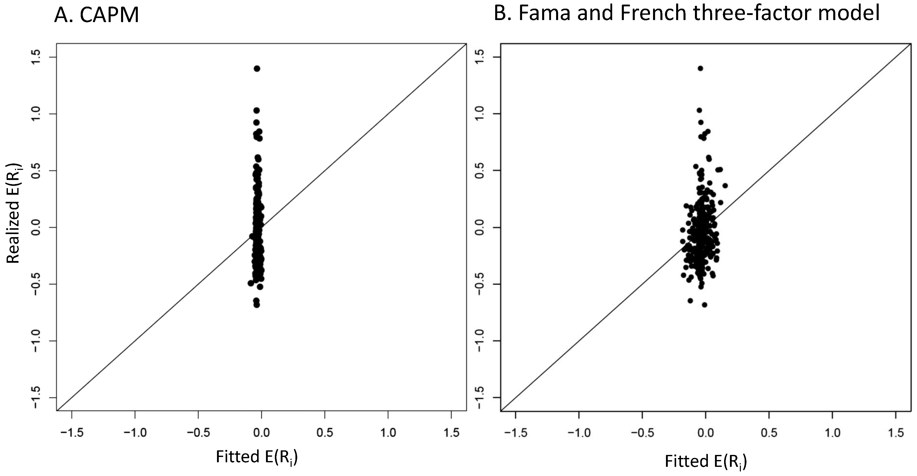
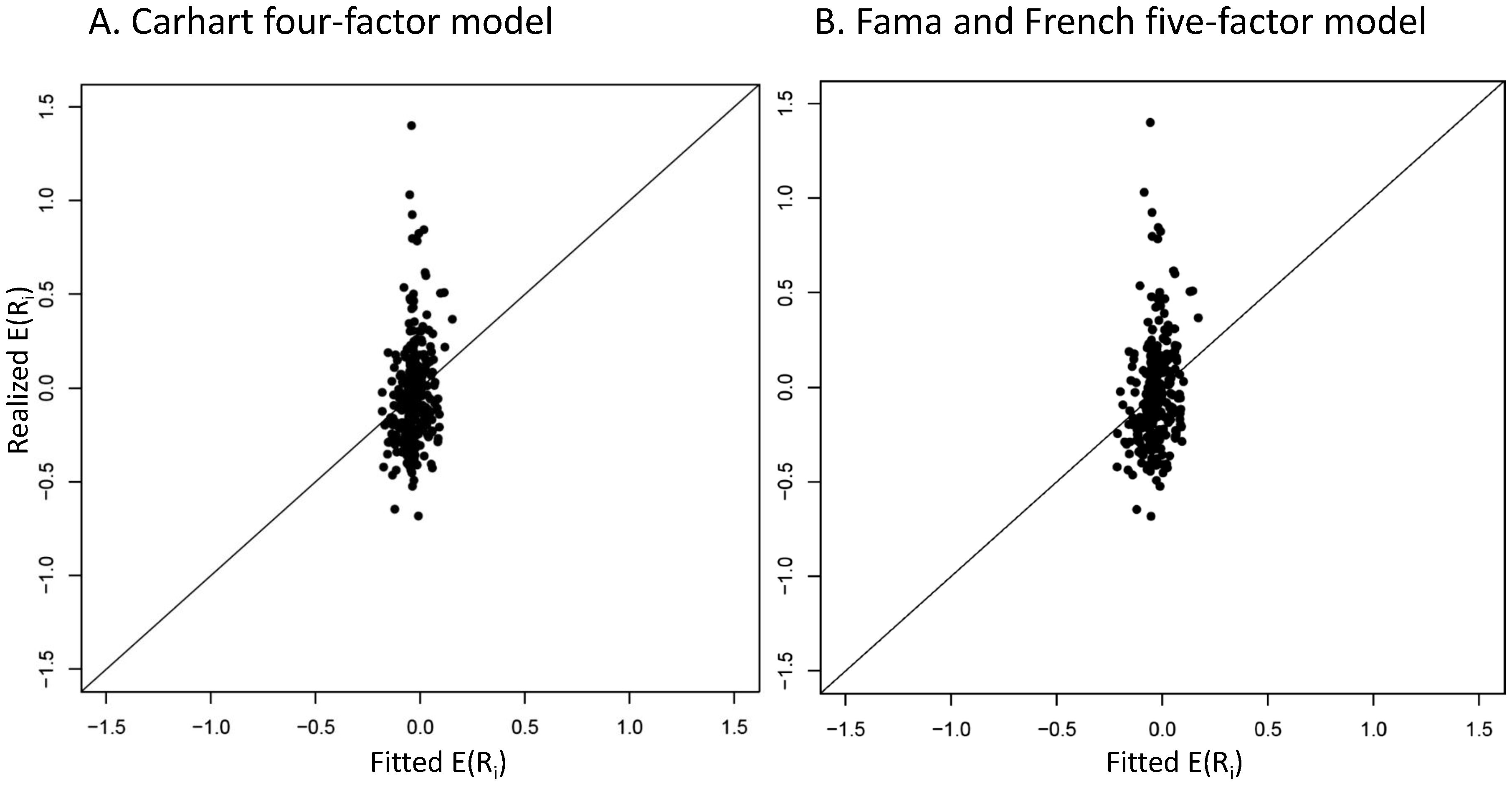
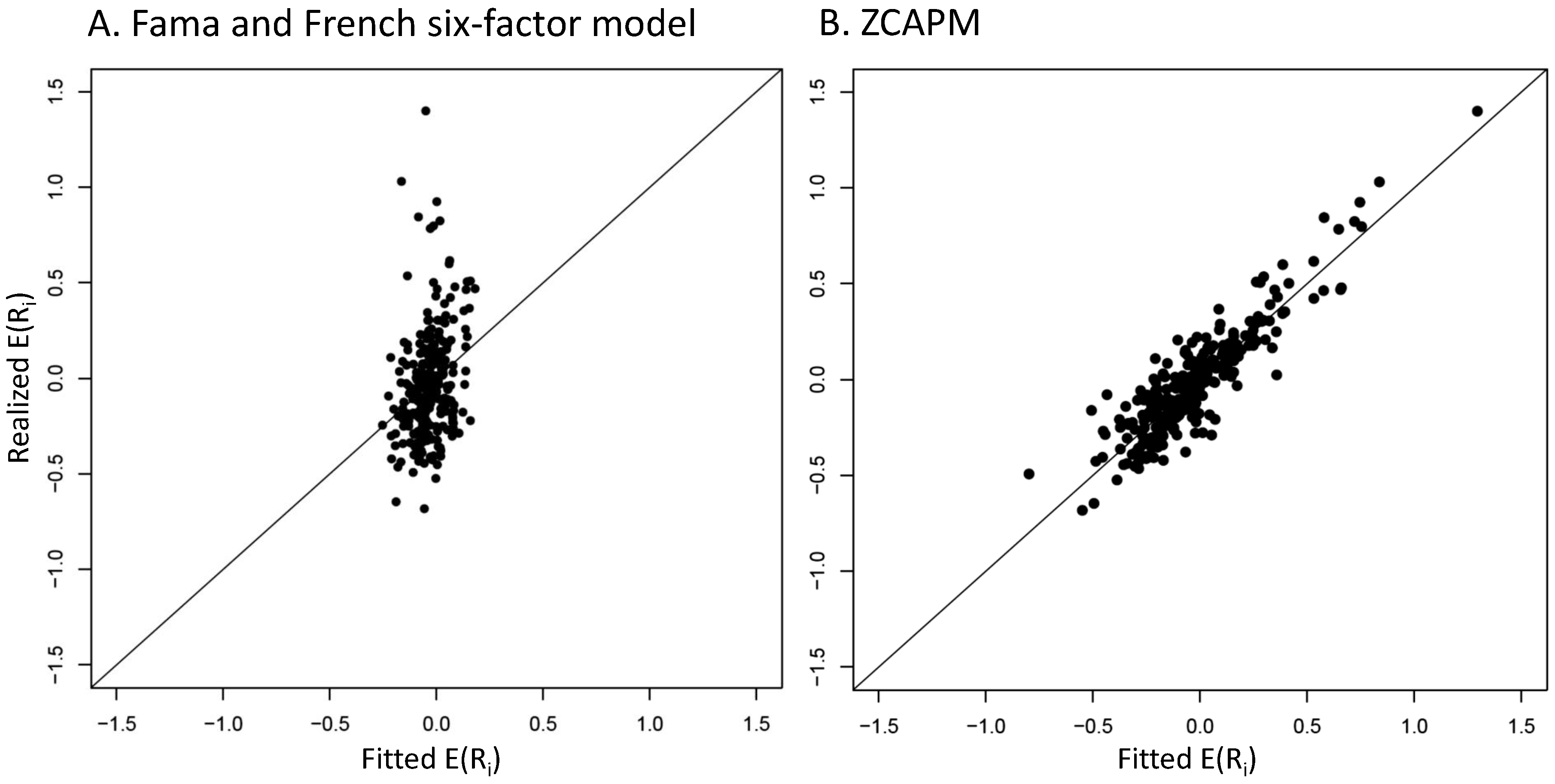
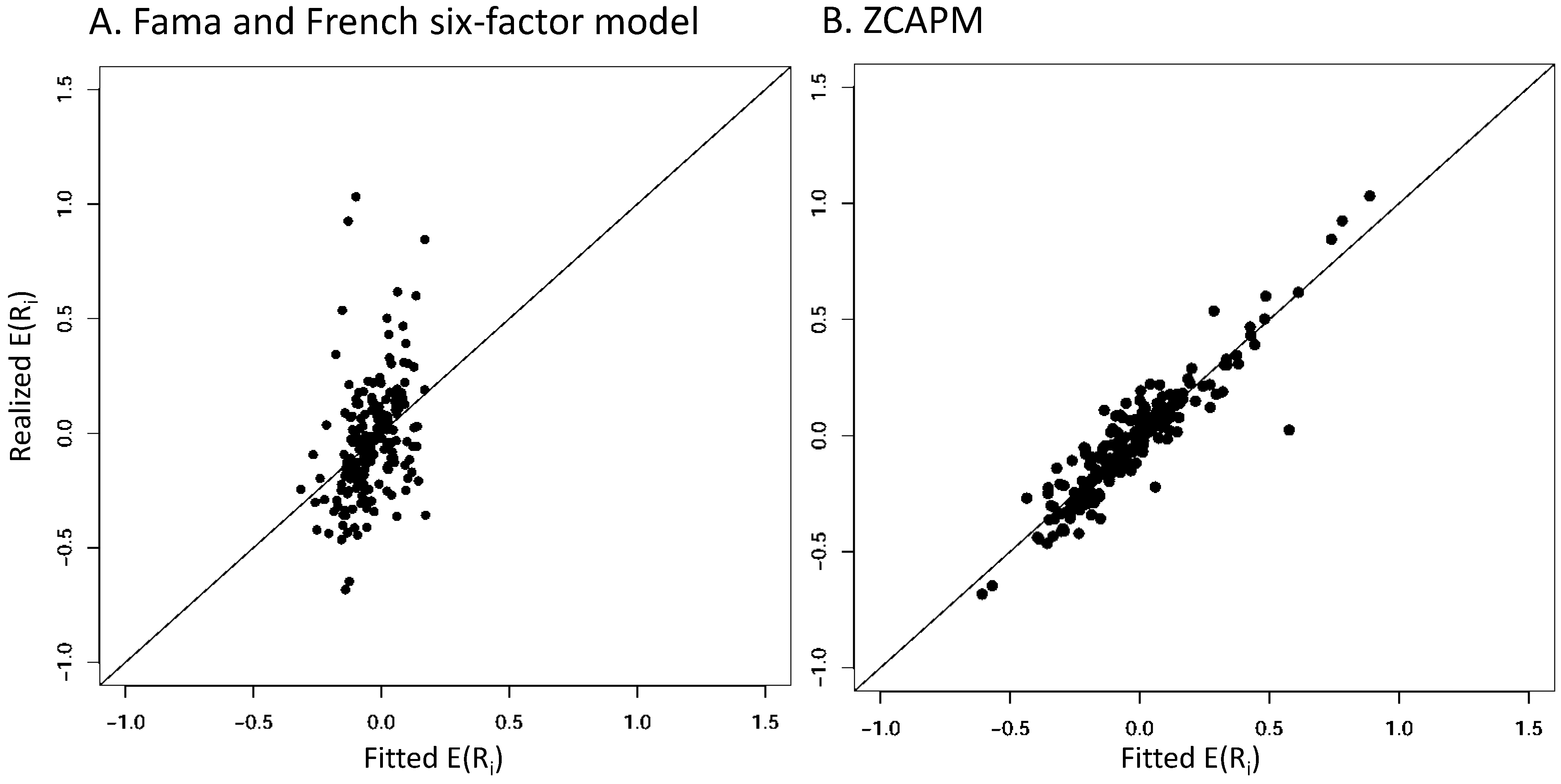
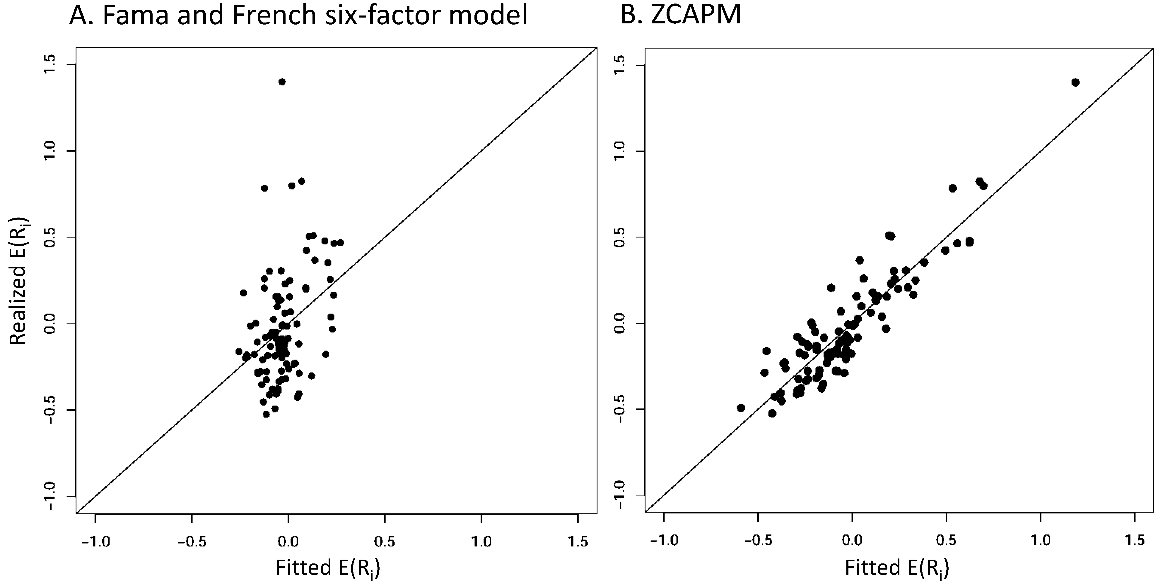
4.2. Graphical Mispricing Error Results

According to Fama and MacBeth (1973), a normative model that helps investors make better return/risk decisions is valid to the extent that it can utilize past information to explain future returns. In line with this logic, Cochrane (1996) and Lettau and Ludvigson (2001) have highlighted the comparative analyses of predicted versus realized (actual) returns to evaluate mispricing errors in asset pricing models. As Cochrane (1996) has asserted, “Expected return pricing errors … are a useful characterization of a model’s performance.” (p. 596). In conducting these analyses, he recommended that “… it is important to examine a model’s ability to explain the expected returns of economically interesting portfolios.” (p. 598). Of course, because anomaly portfolios are difficult for asset pricing models to explain, they are compelling test assets to investigate.

As described earlier, we compute mispricing errors on an out-of-sample basis based on one-month-ahead cross-sectional regressions. Using one year of daily returns for the 286 anomaly portfolios, a time-series regression is run to estimate each asset pricing model and its factor loadings. In the second step, we estimate an out-of-sample (one-month-ahead) cross-sectional regression using one-month-ahead excess returns for anomaly portfolios. By rolling forward one month at a time, this process generates $t=1,\cdots ,582$ cross-sectional regressions from July 1973 to December 2021. In the next month for each portfolio, we utilize the average of the estimated factor prices of risk ${\widehat{\lambda }}_k$ and average estimated loadings for the ith portfolio to compute average fitted excess returns. Lastly, for each asset pricing model, a graph is created with average fitted excess returns plotted against each portfolio’s one-month-ahead average actual excess returns.

Figure 2, Figure 3 and Figure 4 illustrate the average pricing errors of different asset pricing models. In Figure 2, we see that both the CAPM and Fama and French three-factor model exhibit large mispricing errors. Instead of pricing errors lining up on the 45 degree line, they are densely populated around the line in a vertical pattern.

As shown in Figure 3, the Carhart four-factor model and Fama and French five-factor model do not materially improve mispricing. By casual observation, the pricing errors for the 286 anomaly portfolios are large in both models.

Finally, Figure 4 compares the Fama and French six-factor model to the ZCAPM. While the six-factor model improves upon the five-factor model in terms of lower mispricing errors, the ZCAPM makes a quantum leap in pricing. Indeed, no anomaly portfolio lies far off the 45 degree line. This level of out-of-sample pricing is exceptional. One would expect that some anomalies would be difficult to price and, therefore, would be located well off the line. In this case, winsorizing the data to eliminate spurious outliers would be useful to investigate. However, because virtually all of the anomaly portfolios are well explained by the ZCAPM, we did not winsorize the data. It is noteworthy that these mispricing error results are based on out-of-sample tests that employ beta risk and zeta risk estimated in a prior one-year period to compute fitted or predicted returns in the next month. Indeed, future returns are lining up almost exactly with previously estimated systematic risks via the ZCAPM.

The major implication of these graphical analyses is that the 286 anomaly portfolios are anomalous to other asset pricing models but not the ZCAPM. In effect, none of these portfolios appears to be anomalous from the perspective of the ZCAPM. We infer that, in light of these ZCAPM findings, researchers need to expand their search to find long/short stock market anomalies.

4.3. Robustness Tests

As robustness tests, we divide the sample 286 anomalies into two subsamples. The first subsample contains 189 anomalies based on firm characteristics (e.g., size, book-to-market equity, profit, capital investment, etc.). The second subsample includes 97 anomalies based on market characteristics (e.g., momentum, bid-ask spread, trading volume, etc.). Appendix A and Appendix B classify anomalies into these two categories.

Table 3. Out-of-sample Fama–MacBeth cross-sectional tests of 189 anomaly portfolios based on firm characteristics for asset pricing models in the sample period July 1972 to December 2021. Using 189 anomaly portfolios based on firm characteristics (comprising 84 plus 105 anomalous portfolios from A. Y. Chen and Zimmermann (2022) and Jensen et al. (2023), respectively), this table contains results for the sample period July 1972 to December 2021. Based on standard two-step Fama–MacBeth cross-sectional tests, we report out-of-sample (one-month-ahead) estimated market prices of risk denoted ${\widehat{\lambda }}_k$ for the kth factor for the analysis period July 1973 to December 2021. Associated t-statistics are shown in parentheses below estimated prices of risk. The asset pricing models are: CAPM, Fama and French three-factor model (FF3), Carhart four-factor model (C4), Fama and French five-factor model (FF5), Fama and French six-factor model (FF6), and ZCAPM. Factors in these models are denoted as m (CRSP index excess return¹), $\mathit{RD}$ (market return dispersion), $\mathit{SMB}$ (size), $\mathit{HML}$ (value), $\mathit{MOM}$ (momentum), $\mathit{RMW}$ (profit), and $\mathit{CMA}$ (capital investment). The results are shown for the analysis period.

Model	$\widehat{\mathit{\alpha }}$	${\widehat{\mathit{\lambda }}}_{\mathit{m}}$	${\widehat{\mathit{\lambda }}}_{\mathit{RD}}$	${\widehat{\mathit{\lambda }}}_{\mathit{SMB}}$	${\widehat{\mathit{\lambda }}}_{\mathit{HML}}$	${\widehat{\mathit{\lambda }}}_{\mathit{MOM}}$	${\widehat{\mathit{\lambda }}}_{\mathit{RMW}}$	${\widehat{\mathit{\lambda }}}_{\mathit{CMA}}$	${\mathit{R}}^2$
CAPM	−0.07	−0.14							0.08
	(−3.39 ***)	(−0.51)
FF3	−0.09	−0.13		0.06	0.11				0.10
	(−4.48 ***)	(−0.64)		(0.29)	(0.81)
C4	−0.10	−0.36		0.05	0.13	0.08			0.11
	(−5.57 ***)	(−1.73 *)		(0.23)	(0.92)	(0.35)
FF5	−0.12	−0.17		0.10	0.07		0.09	0.22	0.13
	(−6.38 ***)	(−0.84)		(0.54)	(0.50)		(0.72)	(2.14 **)
FF6	−0.13	−0.36		0.09	0.12	0.11	0.13	0.20	0.14
	(−7.55 ***)	(−1.76 *)		(0.49)	(0.85)	(0.50)	(1.07)	(1.94 *)
ZCAPM	−0.01	0.12	0.67						0.86
	(−0.43)	(0.47)	(7.01 ***)

¹ In the ZCAPM, due to using average market excess returns rather than a proxy for market portfolio excess returns, the price of beta risk associated with CRSP index excess returns is denoted ${\widehat{\lambda }}_a$ instead of ${\widehat{\lambda }}_m$ in the other models. Asterisks indicate the level of statistical significance: *—10 percent, **—5 percent, and ***—1 percent.

and

Table 4. Out-of-sample Fama–MacBeth cross-sectional tests of 97 anomaly portfolios based on market characteristics for asset pricing models in the sample period July 1972 to December 2021. Using a total of 97 anomaly portfolios based on market characteristics (comprising 49 plus 48 anomalous portfolios from A. Y. Chen and Zimmermann (2022) and Jensen et al. (2023), respectively), this table contains results for the sample period July 1972 to December 2021. Based on standard two-step Fama–MacBeth cross-sectional tests, we report out-of-sample (one-month-ahead) estimated market prices of risk denoted ${\widehat{\lambda }}_k$ for the kth factor for the analysis period July 1973 to December 2021. Associated t-statistics are shown in parentheses below estimated prices of risk. The asset pricing models are CAPM, Fama and French three-factor model (FF3), Carhart four-factor model (C4), Fama and French five-factor model (FF5), Fama and French six-factor model (FF6), and ZCAPM. Factors in these models are denoted as m (CRSP index excess return¹), $\mathit{RD}$ (market return dispersion), $\mathit{SMB}$ (size), $\mathit{HML}$ (value), $\mathit{MOM}$ (momentum), $\mathit{RMW}$ (profit), and $\mathit{CMA}$ (capital investment). The results are shown for the analysis period.

Model	$\widehat{\mathit{\alpha }}$	${\widehat{\mathit{\lambda }}}_{\mathit{m}}$	${\widehat{\mathit{\lambda }}}_{\mathit{RD}}$	${\widehat{\mathit{\lambda }}}_{\mathit{SMB}}$	${\widehat{\mathit{\lambda }}}_{\mathit{HML}}$	${\widehat{\mathit{\lambda }}}_{\mathit{MOM}}$	${\widehat{\mathit{\lambda }}}_{\mathit{RMW}}$	${\widehat{\mathit{\lambda }}}_{\mathit{CMA}}$	${\mathit{R}}^2$
CAPM	0.00	0.34							0.02
	(−0.10)	(1.48)
FF3	−0.02	0.32		−0.20	0.16				0.06
	(−0.62)	(1.87 *)		(−1.14)	(1.05)
C4	−0.06	0.16		−0.20	0.11	0.31			0.12
	(−2.48 ***)	(0.96)		(−1.22)	(0.82)	(1.52)
FF5	−0.05	0.38		−0.06	0.09		0.31	0.16	0.07
	(−1.94 *)	(2.23 **)		(−0.35)	(0.55)		(1.91 *)	(1.27)
FF6	−0.08	0.18		−0.06	0.10	0.36	0.32	0.05	0.12
	(−3.58 ***)	(1.08)		(−0.40)	(0.73)	(1.72 *)	(2.29 **)	(0.46)
ZCAPM	0.07	0.56	0.69						0.83
	(2.35 ***)	(2.67 ***)	(6.46 ***)

¹ In the ZCAPM, due to using average market excess returns rather than a proxy for market portfolio excess returns, the price of beta risk associated with CRSP index excess returns is denoted ${\widehat{\lambda }}_a$ instead of ${\widehat{\lambda }}_m$ in the other models. Asterisks indicate the level of statistical significance: *—10 percent, **—5 percent, and ***—1 percent.

report the out-of-sample cross-sectional regression results for firm and market characteristic subsamples. In general, the results are similar to those in Table 2 using the combined total sample. For the ZCAPM, the estimated $R^2$ values are 86 percent and 83 percent, respectively, in these two subsamples, which are close to the 84 percent achieved in Table 2. Other models have explanatory power equal to at most 14 percent and 12 percent, respectively. Again the market prices of zeta risk (or ${\widehat{\lambda }}_{RD}$) are highly significant with t-statistics of 7.01 and 6.46, respectively. A few multifactor loadings were significant at 10 percent or 5 percent levels (viz., momentum, profitability, and capital investment); however, they were normally not significant in different multifactor models. These results corroborate our earlier findings for the total sample.

Focusing on the Fama and French six-factor model and ZCAPM, Figure 5 and Figure 6 illustrate the average mispricing errors for the 189 firm-based and 97 market-based anomalies, respectively. The overall results are consistent with those in Figure 4 for the total sample of anomalies. However, comparing these two figures, it appears that mispricing errors are somewhat larger in Figure 6’s market-based anomalies that Figure 5’s firm-based anomalies. Even so, the ZCAPM does a much better job of pricing than the six-factor model.

4.4. What Explains ZCAPM Outperformance?

The clear outperformance of the ZCAPM relative to prominent asset pricing models published in top tier finance journals is impressive. What explains this outperformance? According to KLH, long/short factors in multifactor models are rough measures of cross-sectional market return dispersion. For example, the size factor is long higher yielding small stocks and short lower yielding large stocks. It is likely that small stocks are located in the upper half of the mean-variance investment parabola, whereas large stocks are somewhere in the lower half of the parabola. As the parabola widens (narrows), the size factor experiences higher (lower) returns. This two-sided volatility effect is tantamount to the market return dispersion factor in the ZCAPM. However, the long/short size factor is only a slice or piece of the total market return dispersion (or ${\sigma }_a$) in the ZCAPM.

Other multifactors account for other slices within the total market return dispersion that defines the width or span of the mean-variance parabola. As long/short factors are added to multifactor models, they will gradually converge to the total market return dispersion of the ZCAPM. However, long/short factors tend to be unstable over time. If large stocks and small stocks switch their positions in the parabola, then the size factor would flip from being positively priced to being negatively priced. Some studies have observed this pricing behavior for the size factor. Also, a factor could be significant in one time period but not in other periods as the locations of long and short portfolios in the factor move around in the parabola over time.17

KLH have argued that all multifactors are contained within total market return dispersion. There is no need to use all these factors and look for new factors—the factor zoo is captured by market return dispersion. In turn, the ZCAPM measures their aggregate systematic risk in zeta risk.

An important implication of these insights is that multifactor models are related to the ZCAPM. All multifactor models, including the ZCAPM, employ cross-sectional return dispersion in stock returns to explain asset prices. Moreover, in view of this association, we can link multifactor models to the CAPM, as the ZCAPM is mathematically derived from the zero-beta CAPM. According to KLH, the ZCAPM provides a unifying theory and empirical methodology in the field of asset pricing.

It is interesting that Black (1995) later discussed the second beta factor in his zero-beta CAPM. In this words, the second beta factor is “… the minimum-variance, zero-beta portfolio of risky assets, where beta is defined using whatever market portfolio we use to represent the first factor.” (p. 170). He reasoned as follows:

“When Fama and French say that the line relating expected return and beta is flat, they are just saying that the expected excess return on the second factor is large. If we believe it’s as large as they say, we won’t fool around with their third and fourth factors, for which they give no theory.18 We’ll go for the gold in the second factor!”

(p. 170)

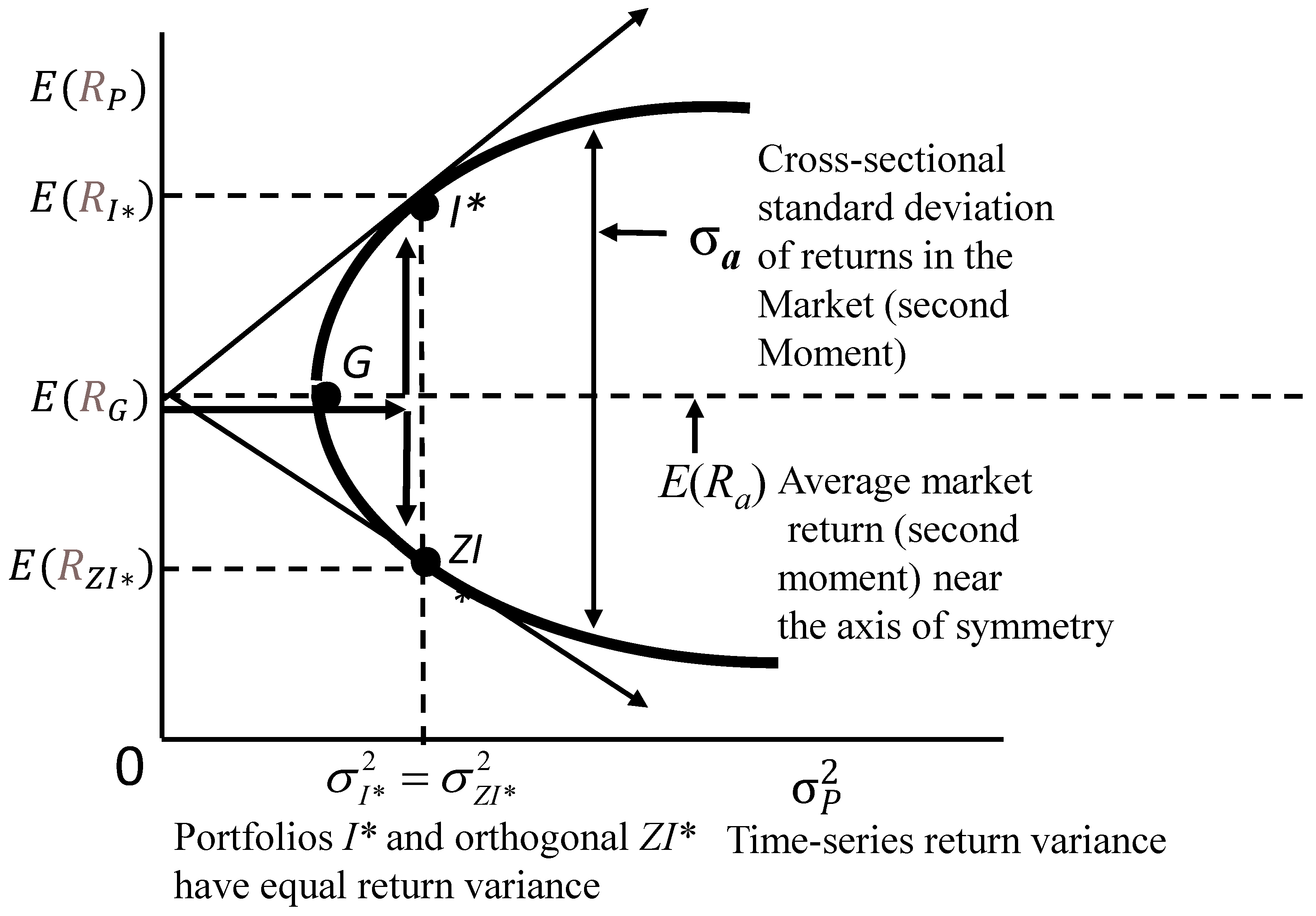
KLH conjectured that market return dispersion corresponds to Black’s second factor. Figure 1 illustrates his second factor as the difference between the returns of an efficient portfolio and inefficient, zero-beta portfolio (with equal return variance), or market return dispersion. It is not necessary to know the expected returns in these two portfolios as their difference corresponds to total market return dispersion. An important policy implication of the ZCAPM relevant to investors is that zeta risk related to market return dispersion is a salient second risk measure (in addition to beta risk associated with the market factor) when evaluating the return performance of stock portfolios.

Finally, the relatively accurate pricing of large numbers of anomaly portfolios by the ZCAPM strongly supports the efficient market hypothesis. As observed by Schwert (2003), Fama and French (2008), Fama (2013), and others, stock market anomalies could be explained by a bad model problem in asset pricing or an inefficient market. The existence of a valid model would confirm that the market is efficient. Echoing this observation, Hou et al. (2020) noted that “… the credibility of the anomalies literature can improve via a close connection with economic theory.” (p. 2072). In this regard, our empirical tests and results of the ZCAPM for anomaly portfolios establish a connection to general equilibrium asset pricing theory.

5. Conclusions

This paper sought to compare the ability of different asset pricing models to explain stock market anomaly portfolio returns. We employed a large dataset of 286 anomaly portfolios provided by A. Y. Chen and Zimmermann (2022) and Jensen et al. (2023). Anomalies are economically interesting due to the fact that they are difficult for asset pricing models to explain.

Surprisingly, virtually all of the anomaly portfolios were well explained by the ZCAPM, a recent model proposed by Kolari et al. (2021). In stark contrast, the CAPM as well as a number of prominent multifactor models could not explain anomaly portfolio returns for the most part. Mispricing errors were large for the latter models compared to relatively small pricing errors for the ZCAPM. Robustness tests of subsamples of firm- and market-based anomalies confirmed these findings.

We conclude that, given the ZCAPM, long/short stock market anomaly portfolios under study are no longer anomalies. Given the ability of the ZCAPM to explain large datasets of anomalies, our findings support the efficient markets hypothesis. The scope of our study is limited to U.S. stock market anomalies. Further research is recommended on stock market anomalies in other countries as well as other classes of assets, including bonds, commodities, and other asset traded on a daily basis. Also, an important implication for future research is the search to identify long/short stocks portfolios not explained by the ZCAPM. Perhaps behavioral explanations of these anomalies are possible.

References

1. Ang, A., Hodrick, R. J., Xing, Y., & Zhang, X. (2006). The cross-section of volatility and expected returns. Journal of Finance, 61, 259–299. [Google Scholar] [CrossRef]
2. Ang, A., Madhaven, A., & Sobczyk, A. (2017). Estimating time-varying factor exposures. Financial Analysts Journal, 73, 41–54. [Google Scholar] [CrossRef]
3. Angelidis, T., Sakkas, A., & Tessaromatis, N. (2015). Stock market dispersion, the business cycle and expected factor returns. Journal of Banking and Finance, 59, 256–279. [Google Scholar] [CrossRef]
4. Asquith, D., Jones, J., & Kieschnick, R. (1998). Evidence on price stabilization and underpricing in early IPO returns. Journal of Finance, 53, 1759–1773. [Google Scholar] [CrossRef]
5. Back, K., Kapadia, N., & Ostdiek, B. (2013). Slopes as factors: Characteristic pure plays. Working paper. Rice University. [Google Scholar]
6. Back, K., Kapadia, N., & Ostdiek, B. (2015). Testing factor models on characteristic and covariance pure plays. Working paper. Rice University. [Google Scholar]
7. Bansal, R., & Yaron, A. (2004). Risks for the long run: A potential resolution of asset pricing puzzles. Journal of Finance, 59, 1481–1509. [Google Scholar] [CrossRef]
8. Barberis, N., Shleifer, A., & Vishny, R. (1998). A model of investor sentiment. Journal of Financial Economics, 49, 307–343. [Google Scholar] [CrossRef]
9. Bartram, S. M., & Grinblatt, M. (2018). Agnostic fundamental analysis works. Journal of Financial Economics, 128, 125–147. [Google Scholar] [CrossRef]
10. Bekaert, G., Engstrom, E., & Ermolov, A. (2023). The variance risk premium in equilibrium models. Review of Finance, 27, 1977–2014. [Google Scholar] [CrossRef]
11. Bekaert, G., & Harvey, C. (1997). Emerging equity market volatility. Journal of Financial Economics, 43, 29–77. [Google Scholar] [CrossRef]
12. Black, F. (1972). Capital market equilibrium with restricted borrowing. Journal of Business, 45, 444–454. [Google Scholar] [CrossRef]
13. Black, F. (1995). Estimating expected return. Financial Analysts Journal, 49, 36–38. [Google Scholar] [CrossRef]
14. Bo, C. B., & Batzoglou, S. (2008). What is the expectation maximization algorithm? Nature Biotechnology, 26, 897–899. [Google Scholar]
15. Bowles, B., Reed, A. V., Ringgenberg, M. C., & Thornock, J. R. (2023). Anomaly time. Journal of Finance, 79, 3543–3579. [Google Scholar] [CrossRef]
16. Carhart, M. M. (1997). On persistence in mutual fund performance. Journal of Finance, 52, 57–82. [Google Scholar] [CrossRef]
17. Chen, A. Y., & Velikov, M. (2023). Zeroing in on the expected returns of anomalies. Journal of Financial and Quantitative Analysis, 58, 968–1004. [Google Scholar] [CrossRef]
18. Chen, A. Y., & Zimmermann, T. (2020). Publication bias and the cross-section of stock returns. Review of Asset Pricing Studies, 10, 249–289. [Google Scholar] [CrossRef]
19. Chen, A. Y., & Zimmermann, T. (2022). Open source cross-sectional asset pricing. Critical Finance Review, 11, 207–264. [Google Scholar] [CrossRef]
20. Chen, N.-F. (1983). Empirical tests of the theory of arbitrage pricing. Journal of Finance, 38, 1393–1414. [Google Scholar] [CrossRef]
21. Chen, Y., Cliff, M., & Zhao, H. (2017). Hedge funds: The good, the bad, and the lucky. Journal of Financial and Quantitative Analysis, 52, 1081–1109. [Google Scholar] [CrossRef]
22. Chordia, T., Goyal, A., & Saretto, A. (2020). Anomalies and false rejections. Review of Financial Studies, 33, 2134–2179. [Google Scholar] [CrossRef]
23. Chordia, T., Subrahmanyam, A., & Tong, Q. (2014). Have capital market anomalies attenuated in the recent era of high liquidity and trading activity? Journal of Accounting and Economics, 58, 41–58. [Google Scholar] [CrossRef]
24. Christie, W., & Huang, R. (1994). The changing functional relation between stock returns and dividend yields. Journal of Empirical Finance, 1, 161–191. [Google Scholar] [CrossRef]
25. Cochrane, J. H. (1996). A cross-sectional test of an investment-based asset pricing model. Journal of Political Economy, 104, 572–621. [Google Scholar] [CrossRef]
26. Cochrane, J. H. (2011). Presidential address: Discount rates. Journal of Finance, 56, 1047–1108. [Google Scholar] [CrossRef]
27. Connolly, R., & Stivers, C. (2003). Momentum and reversals in equity index returns during periods of abnormal turnover and return dispersion. Journal of Finance, 58, 1521–1556. [Google Scholar] [CrossRef]
28. Cooper, M., Gulen, H., & Ion, M. (2024). The use of asset growth in empirical asset pricing models. Journal of Financial Economics, 151, 103746. [Google Scholar] [CrossRef]
29. Copeland, T. E., & Weston, J. F. (1980). Financial theory and corporate policy. Addison-Wesley Publishing Company. [Google Scholar]
30. Daniel, K., Hirshleifer, D., & Subrahmanyam, A. (1997). A theory of overconfidence, self-attribution, and security market under- and over-reactions [Unpublished working paper]. University of Michigan. [Google Scholar]
31. DeBondt, W. F. M., & Thaler, R. H. (1987). Further evidence on investor overreaction and stock market seasonality. Journal of Finance, 42, 557–581. [Google Scholar] [CrossRef]
32. Demirer, R., & Jategaonkar, S. P. (2013). The conditional relation between dispersion and return. Review of Financial Economics, 22, 125–134. [Google Scholar] [CrossRef]
33. Dempster, A. P., Laird, N. M., & Rubin, D. B. (1977). Maximum likelihood from incomplete data via the EM algorithm. Journal of the Royal Statistical Society, 39, 1–38. [Google Scholar] [CrossRef]
34. Detzel, A., Duarte, J., Kamara, A., & Siegel, S. (2023). The cross-section of volatility and expected returns: Then and now. Critical Finance Review, 12, 9–56. [Google Scholar] [CrossRef]
35. Engelberg, J., McLean, R. D., & Pontiff, J. (2018). Anomalies and news. Journal of Finance, 73, 1972–2001. [Google Scholar]
36. Fama, E. F. (1970). Efficient capital markets: A review of theory and empirical work. Journal of Finance, 25, 383–417. [Google Scholar] [CrossRef]
37. Fama, E. F. (2013). Two pillars of asset pricing. American Economic Review, 104, 1467–1485. [Google Scholar] [CrossRef]
38. Fama, E. F., & French, K. R. (1992). The cross-section of expected stock returns. Journal of Finance, 47, 427–465. [Google Scholar]
39. Fama, E. F., & French, K. R. (1993). Common risk factors in the returns on stocks and bonds. Journal of Financial Economics, 33, 3–56. [Google Scholar] [CrossRef]
40. Fama, E. F., & French, K. R. (1996). The CAPM is wanted, dead or alive. Journal of Finance, 51, 1947–1958. [Google Scholar] [CrossRef]
41. Fama, E. F., & French, K. R. (1998). Market efficiency, long-term returns, and behavioral finance. Journal of Financial Economics, 49, 283–306. [Google Scholar] [CrossRef]
42. Fama, E. F., & French, K. R. (2008). Dissecting anomalies. Journal of Finance, 63, 1653–1678. [Google Scholar] [CrossRef]
43. Fama, E. F., & French, K. R. (2015). A five-factor asset pricing model. Journal of Financial Economics, 116, 1–22. [Google Scholar] [CrossRef]
44. Fama, E. F., & French, K. R. (2018). Choosing factors. Journal of Financial Economics, 128, 234–252. [Google Scholar] [CrossRef]
45. Fama, E. F., & MacBeth, J. D. (1973). Risk, return, and equilibrium: Empirical tests. Journal of Political Economy, 81, 607–636. [Google Scholar] [CrossRef]
46. Ferson, W. E. (2019). Empirical asset pricing: Models and methods. The MIT Press. [Google Scholar]
47. Garcia, R., Mantilla-Garcia, D., & Martellini, L. (2014). A model-free measure of aggregate idiosyncractic volatility and the prediction of market returns. Journal of Financial and Quantitative Analysis, 49, 1133–1165. [Google Scholar] [CrossRef]
48. Gibbons, M. R., Ross, S. A., & Shanken, J. (1989). A test of the efficiency of a given portfolio. Econometrica, 57, 1121–1152. [Google Scholar] [CrossRef]
49. Gomes, J., Kogan, L., & Zhang, L. (2003). Equilibrium cross section of returns. Journal of Political Economy, 111, 693–732. [Google Scholar] [CrossRef]
50. Green, J., Hand, J. R., & Zhang, F. (2017). The characteristics that provide independent information about average US monthly stock returns. Review of Financial Studies, 30, 4389–4436. [Google Scholar] [CrossRef]
51. Green, J., Hand, J. R., & Zhang, X. F. (2013). The supraview of return predictive signals. Review of Accounting Studies, 18, 692–730. [Google Scholar] [CrossRef]
52. Harvey, C. R., & Liu, Y. (2016). Rethinking performance evaluation. Working paper no. 22134. National Bureau of Economic Research, Inc. [Google Scholar]
53. Harvey, C. R., Liu, Y., & Zhu, H. (2016). … and the cross-section of expected returns. Review of Financial Studies, 29, 5–68. [Google Scholar] [CrossRef]
54. Hou, K., Xue, C., & Zhang, L. (2015). Digesting anomalies: An investment approach. Review of Financial Studies, 28, 650–705. [Google Scholar] [CrossRef]
55. Hou, K., Xue, C., & Zhang, L. (2020). Replicating anomalies. Review of Financial Studies, 33, 2019–2133. [Google Scholar] [CrossRef]
56. Jacobs, H., & Müller, S. (2020). Anomalies cross the globe: Once public, no longer existent? Journal of Financial Economics, 135, 213–230. [Google Scholar] [CrossRef]
57. Jagannathan, R., & Wang, Z. (1996). The conditional CAPM and the cross-section of asset returns. Journal of Finance, 51, 3–53. [Google Scholar]
58. Jensen, T. I., Kelly, B., & Pedersen, L. H. (2023). Is there a replication crisis in finance? Journal of Finance, 78, 2465–2518. [Google Scholar] [CrossRef]
59. Jiang, X. (2010). Return dispersion and expected returns. Financial Markets and Portfolio Management, 24, 107–135. [Google Scholar] [CrossRef]
60. Jones, P. N., & McLachlan, G. J. (1990). Algorithm AS 254: Maximum likelihood estimation from grouped and truncated data with finite normal mixture models. Applied Statistics, 39, 273–282. [Google Scholar] [CrossRef]
61. Kahneman, D., & Tversky, A. (1979). Prospect theory: An analysis of decision under risk. Econometrica, 47, 263–291. [Google Scholar] [CrossRef]
62. Kolari, J. W., Huang, J. Z., Butt, H. A., & Liao, H. (2022). International tests of the ZCAPM asset pricing model. Journal of International Financial Markets, Institutions &Money, 79, 101607. [Google Scholar]
63. Kolari, J. W., Huang, J. Z., Liu, W., & Liao, H. (2022). Further tests of the ZCAPM asset pricing model. Journal of Risk and Financial Management, 15, 137. [Google Scholar] [CrossRef]
64. Kolari, J. W., Huang, J. Z., Liu, W., & Liao, H. (2023a, March 8–11). A cross-sectional asset pricing test of model validity. Annual Meetings of the Southwestern Finance Association, Las Vegas, NV, USA. Available online: https://papers.ssrn.com/sol3/papers.cfm?abstract_id=4203990 (accessed on 1 April 2025).
65. Kolari, J. W., Huang, J. Z., Liu, W., & Liao, H. (2023b, July 2–6). The alpha force: Testing missing asset pricing factors. Annual Meetings of the Western Economic Association International, San Diego, CA, USA. [Google Scholar]
66. Kolari, J. W., Huang, J. Z., Liu, W., & Liao, H. (2025a, February 12–14). A quantum leap in asset pricing: Explaining anomalyous returns. Annual Meetings of the Southwestern Finance Association, San Antonio, TX, USA. [Google Scholar]
67. Kolari, J. W., Huang, J. Z., Liu, W., & Liao, H. (2025b). Asset pricing models and market efficiency: Using machine Learning to explain stock market anomalies. Palgrave Macmillan. [Google Scholar]
68. Kolari, J. W., Liu, W., & Huang, J. Z. (2021). A new model of capital asset prices: Theory and evidence. Palgrave Macmillan. [Google Scholar]
69. Kolari, J. W., Liu, W., & Pynnonen, S. (2024). Professional investment portfolio management: Boosting performance with machine-made portfolios and stock market evidence. Palgrave Macmillan. [Google Scholar]
70. Lettau, M., & Ludvigson, S. (2001). Consumption, aggregate wealth, and expected stock returns. Journal of Finance, 56, 815–849. [Google Scholar] [CrossRef]
71. Lettau, M., & Pelger, M. (2020). Factors that fit the time series and cross-section of stock returns. Review of Financial Studies, 33, 2274–2325. [Google Scholar] [CrossRef]
72. Linnainmaa, J., & Roberts, M. (2018). The history of the cross-section of stock returns. Review of Financial Studies, 31, 2606–2649. [Google Scholar] [CrossRef]
73. Lintner, J. (1965). The valuation of risk assets and the selection of risky investments in stock portfolios and capital budgets. Review of Economics and Statistics, 47, 13–37. [Google Scholar] [CrossRef]
74. Liu, W. (2013). A new asset pricing model based on the zero-beta CAPM: Theory and evidence [Doctoral dissertation, Texas A&M University]. [Google Scholar]
75. Liu, W., Kolari, J. W., & Huang, J. Z. (2012, October 17–20). A new asset pricing model based on the zero-beta CAPM. 2012 Annual Meetings of the Financial Management Association, Atlanta, GA, USA. [Google Scholar]
76. Liu, W., Kolari, J. W., & Huang, J. Z. (2019). Creating superior investment portfolios. Working paper. Texas A&M University. [Google Scholar]
77. Liu, W., Kolari, J. W., & Huang, J. Z. (2020, November 18–21). Return dispersion and the cross-section of stock returns. Annual Meetings of the Southern Finance Association, Palm Springs, CA, USA. [Google Scholar]
78. Loungani, P., Rush, M., & Tave, W. (1990). Stock market dispersion and unemployment. Journal of Monetary Economics, 25, 367–388. [Google Scholar] [CrossRef]
79. Lu, X., Stambaugh, R. F., & Yuan, Y. (2018). Anomalies abroad: Beyond data mining. Working paper. Shanghai Jiao Tong University. [Google Scholar]
80. Markowitz, H. M. (1952). Portfolio selection. Journal of Finance, 7, 77–91. [Google Scholar]
81. Markowitz, H. M. (1959). Portfolio selection: Efficient diversification of investments. John Wiley & Sons. [Google Scholar]
82. McLachlan, G. J., & Krishnan, T. (2008). The EM algorithm and extensions (2nd ed.). John Wiley & Sons. [Google Scholar]
83. McLachlan, G. J., & Peel, D. (2000). Finite mixture models. Wiley Interscience. [Google Scholar]
84. McLean, R. D., & Pontiff, J. (2016). Does academic publication destroy predictability? Journal of Finance, 71, 5–32. [Google Scholar] [CrossRef]
85. Mossin, J. (1966). Equilibrium in a capital asset market. Econometrica, 34, 768–783. [Google Scholar] [CrossRef]
86. Novy-Marx, R., & Velikov, M. (2016). A taxonomy of anomalies and their trading costs. Review of Financial Studies, 29, 104–147. [Google Scholar] [CrossRef]
87. Pastor, L., & Veronesi, P. (2009). Technological revolutions and stock prices. American Economic Review, 99, 1451–1483. [Google Scholar] [CrossRef]
88. Schwert, G. W. (2003). Anomalies and market efficiency. In G. M. Constantinides, M. Harris, & R. Stulz (Eds.), Handbook of the economics of finance (pp. 939–974). North-Holland. [Google Scholar]
89. Sharpe, W. F. (1964). Capital asset prices: A theory of market equilibrium under conditions of risk. Journal of Finance, 19, 425–442. [Google Scholar]
90. Shiller, R. J. (1981). Do stock prices move too much to be justified by subsequent changes in dividends. American Economic Review, 71, 421–436. [Google Scholar]
91. Stambaugh, R. F., & Yuan, Y. (2017). Mispricing factors. Review of Financial Studies, 30, 1270–1315. [Google Scholar] [CrossRef]
92. Stivers, C. (2003). Firm-level return dispersion and the future volatility of aggregate stock market returns. Journal of Financial Markets, 6, 389–411. [Google Scholar] [CrossRef]
93. Thaler, R. H. (1999). The end of behavioral finance. Financial Analysts Journal, 55, 12–17. [Google Scholar] [CrossRef]
94. Treynor, J. L. (1961). Market value, time, and risk [Unpublished manuscript].
95. Treynor, J. L. (1962). Toward a theory of market value of risky assets [Unpublished manuscript].
96. Zhang, L. (2005). The value premium. Journal of Finance, 60, 67–103. [Google Scholar] [CrossRef]
Figure 1. Locating orthogonal portfolios I and Z I on the mean-variance parabola. Source: Adapted from Kolari et al. (2021, Figure 3.2, p. 59).
Jrfm 18 00362 g001
Figure 2. Out-of-sample cross-sectional CAPM (Panel A) and Fama and French three-factor model (Panel B) mispricing errors comparing average one-month-ahead realized excess returns in percent (Y-axis) to average one-month-ahead predicted (fitted) excess returns in percent (X-axis) for 286 portfolios in the total sample of anomalies. The analysis period is July 1973 to December 2021.
Jrfm 18 00362 g002
Figure 3. Out-of-sample cross-sectional Carhart four-factor model (Panel A) and Fama and French five-factor model (Panel B) mispricing errors comparing average one-month-ahead realized excess returns in percent (Y-axis) to average one-month-ahead predicted (fitted) excess returns in percent (X-axis) for 286 portfoliosin the total sample of anomalies. The analysis period is July 1973 to December 2021.
Jrfm 18 00362 g003
Figure 4. Out-of-sample cross-sectional Fama and French six-factor model (Panel A) and ZCAPM (Panel B) mispricing errors comparing average one-month-ahead realized excess returns in percent (Y-axis) to average one-month-ahead predicted (fitted) excess returns in percent (X-axis) for 286 portfolios in the total sample of anomalies. The analysis period is July 1973 to December 2021.
Jrfm 18 00362 g004
Figure 5. Out-of-sample cross-sectional Fama and French six-factor model (Panel A) and ZCAPM (Panel B) mispricing errors comparing average one-month-ahead realized excess returns in percent (Y-axis) to average one-month-ahead predicted (fitted) excess returns in percent (X-axis) for 189 portfolios based on firm characteristics. The analysis period is July 1973 to December 2021.
Jrfm 18 00362 g005
Figure 6. Out-of-sample cross-sectional Fama and French six-factor model (Panel A) and ZCAPM (Panel B) mispricing errors comparing average one-month-ahead realized excess returns in percent (Y-axis) to average one-month-ahead predicted (fitted) excess returns in percent (X-axis) for 97 portfolios based on market characteristics. The analysis period is July 1973 to December 2021.
Jrfm 18 00362 g006