

Finite Mixture at Quantiles and Expectiles


Abstract
1. Introduction
2. Methods: The Finite Mixture Estimator
3. Method: The FM Estimator in the Tails
3.1. FM-Expectiles
3.2. FM-Quantile
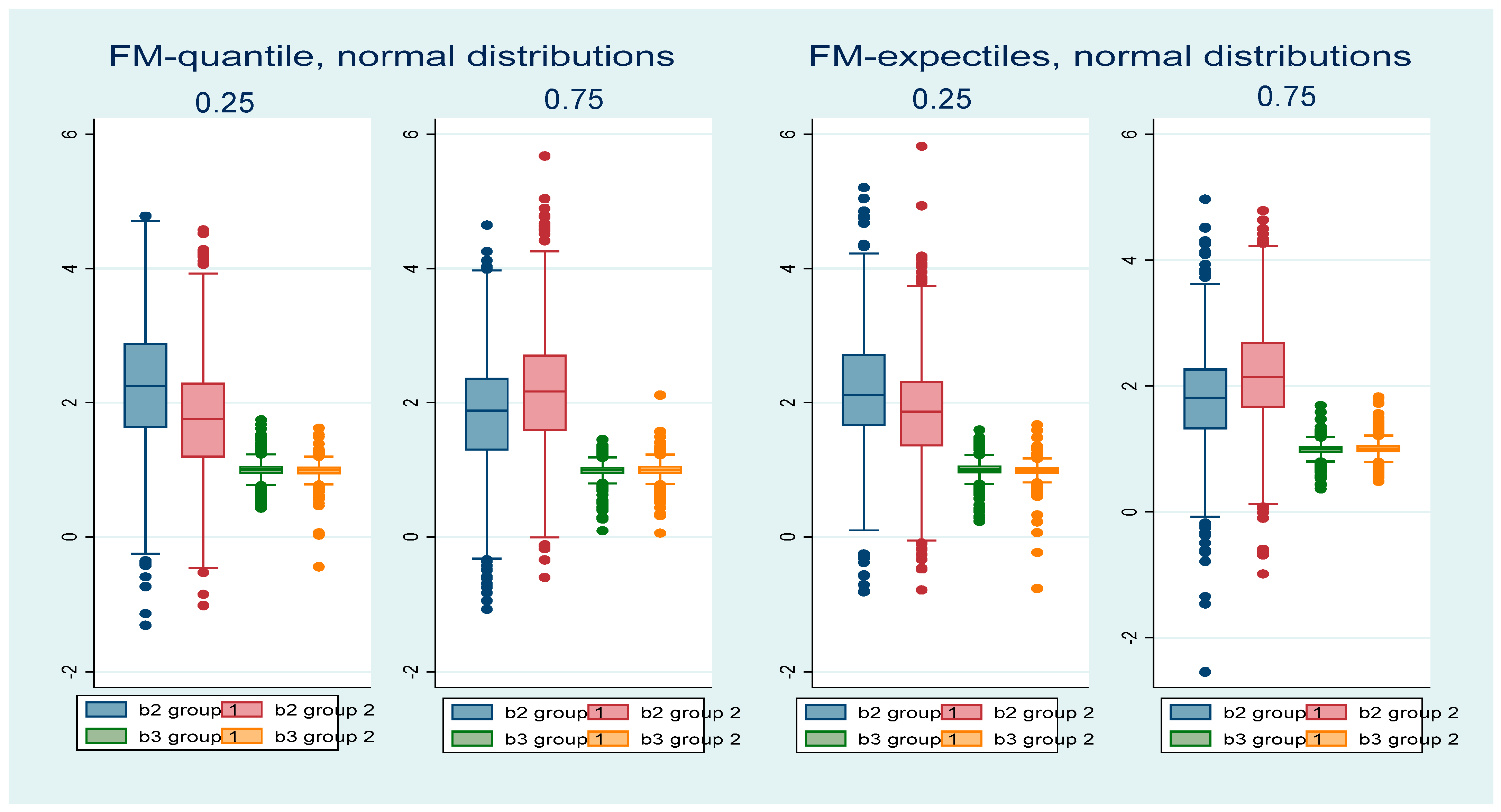
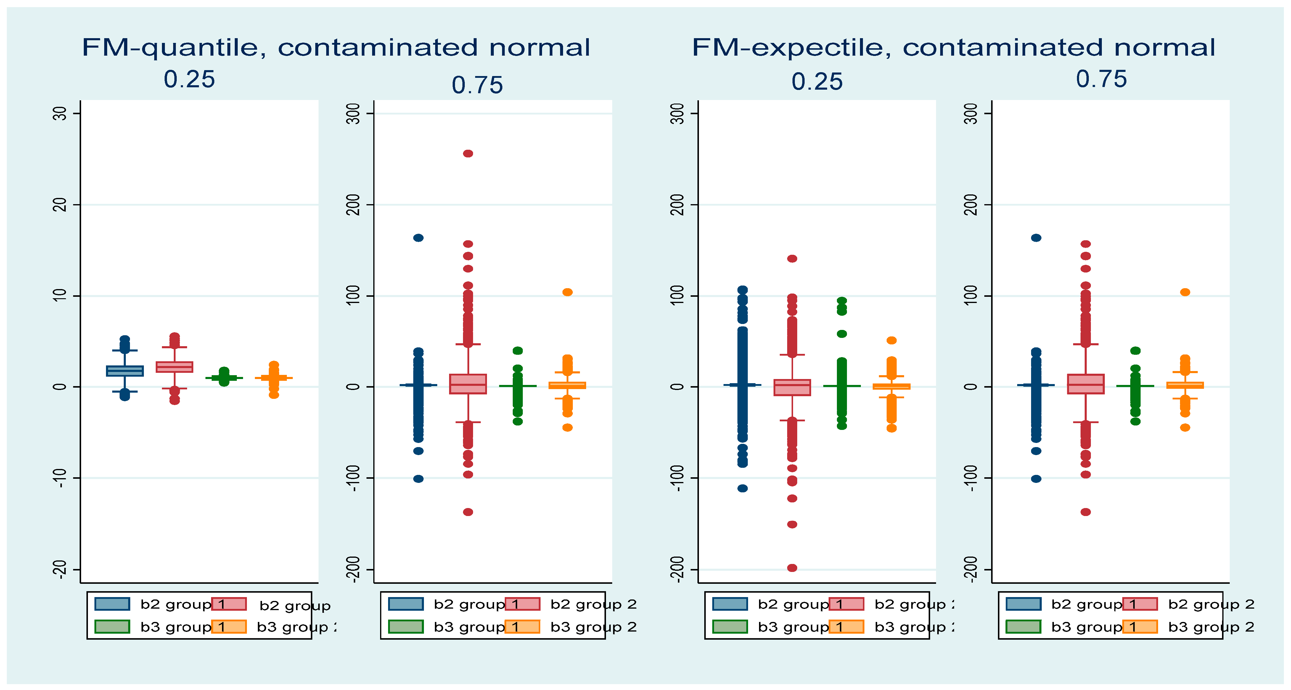
4. Simulations
5. Simulation Results
6. Case Studies
6.1. School Data
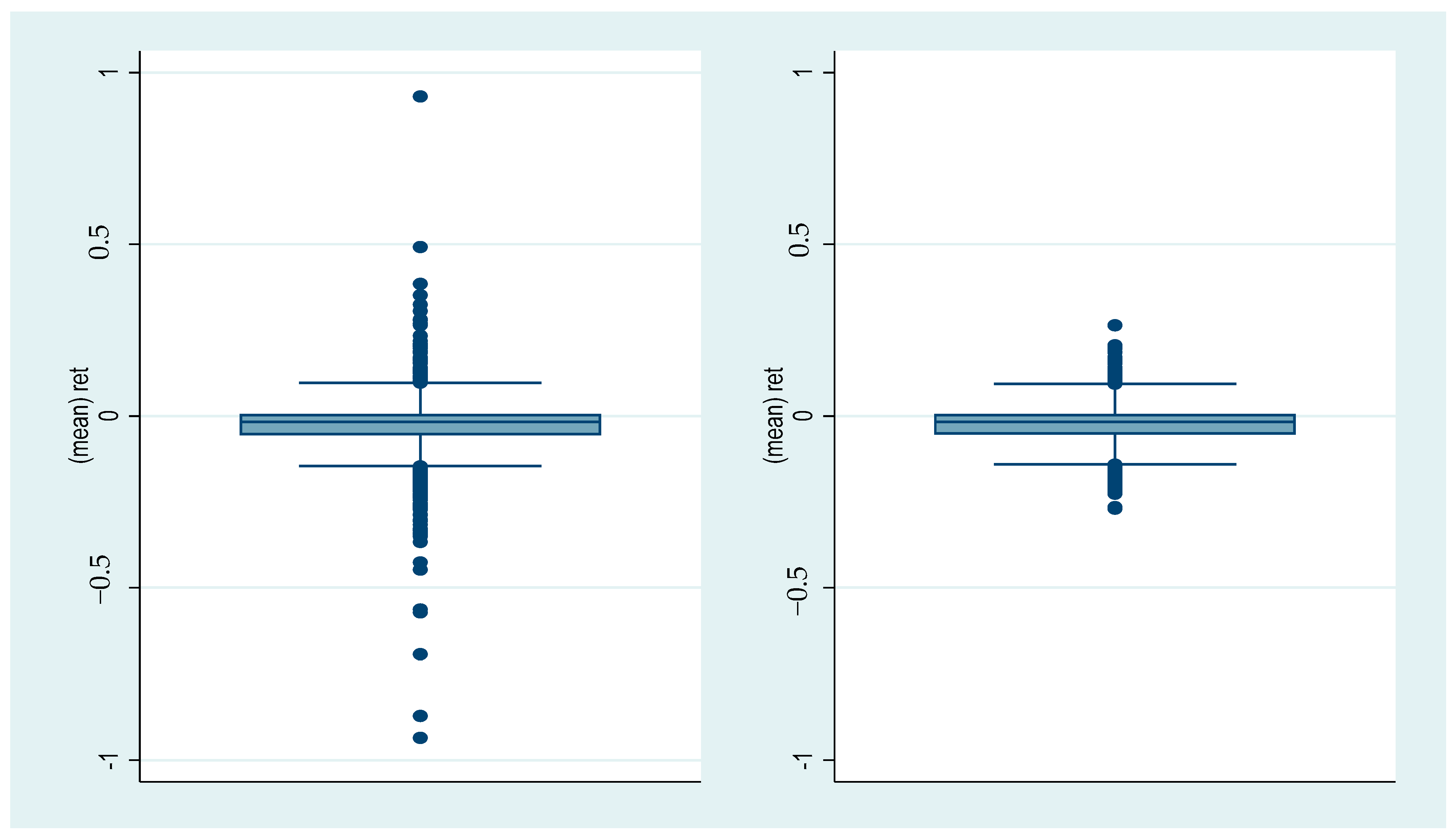
6.2. Financial Data
7. Conclusions
Funding
Institutional Review Board Statement
Informed Consent Statement
Data Availability Statement
Conflicts of Interest
Appendix A. Stata Codes
| reg y x1 x2 | |
| predict resols, resid | |
| *FM at the mean | |
| fmm 2: regress y x1 x2 | |
| *Akaike and log likelihood | |
| estat ic | |
| *probability to belong to a group | |
| estat lcprob | |
| *expectile regression and definition of weights | *first quartile regression weights |
| reg y x1 x2 + | qreg y x1 x2, q(0.25) +++ |
| gen eweight = 1 | predict qres, resid |
| scalar tau = 0.25 | gen qweight = 0.25 if qres > 0 & qres!=. |
| gen wy = eweight*y | replace qweight = 0.75 if qres < 0 & qres!=. |
| gen wx1 = eweight*x1 | |
| gen wx2 = eweight*x2 | |
| forvalues i = 1(1)8 { | |
| predict resid, resid | |
| replace eweight = 2*tau if resid >= 0 | |
| replace eweight = 2*(1-tau) if resid < 0 | |
| replace wy = eweight*y | |
| replace wx1 = eweight*x1 | |
| replace wx2 = eweight*x2 | |
| reg wy wx1 wx2 ++ | |
| drop resid | |
| } | |
| *expectile FM | *quantile FM |
| fmm 2: regress y x1 x2 [pw = eweight] | fmm 2: regress y x1 x2 [pw = qweight] |
| estat ic | estat ic |
| estat lcprob | estat lcprob |
| + can be replaced by logit d x1 x2 | |
| ++ can be replaced by logit wd wx1 wx2 | +++ can be replaced by lqreg qd qx1 qx2 |
| where d is a location dummy assuming value equal to 1 at the chosen expectile/quantile, zero otherwise. | |
| To select the variables defining the group probabilities the FM code becomes | |
| fmm 2, lcprob (z1 z2): regress y x1 x2 [pw = weight] | |
| where z1 and z2 are the explanatory variables defining the group probability. They can or cannot differ from the variables of the regression model. The weight within square brackets is qweight or eweight depending on the selected estimator, FM-quantile or FM-expectile. | |
| 1 | The variables defining the group probability could differ from the variables defining the regression model. In the case studies, the explanatory variables of and coincide. However, the financial model has been re-estimated by setting lagged variables as predictors of group probability in xiq. |
| 2 | The stata code to compute the weights in the expectile logistic regression of Equation (5) is logit eweight-depvar eweight-indepvar within the iterative loop that computes the location expectile weights; eweight are defined by = or = 1 − as in (5) and they modify the regression variables into eweight-depvar and eweight-indepvar, as in (6) (see the Appendix A). |
| 3 | In the expectile case, the regression code to compute (6) is reg eweight-depvar eweight-indepvar within the iterative loop that computes the location weights (see the Appendix A). |
| 4 | The stata code in the quantile regression case of Equation (7) at the quantile is qreg depvar indepvar, q(), and the residuals allow us to define the quantile weights (see the Appendix A). |
| 5 | In the quantile case, the stata code at the θ quantile is lqreg depvar indepvar, q(θ) (Orsini & Bottai, 2011), and the residuals allow us to define the weights (see the Appendix A). |
| 6 | The simulations and all the empirical analyses are implemented in Stata, version 15. |
| 7 | We compute only FM-quantile for comparability’s sake. |
| 8 | The weights can be determined starting from the quantile/expectile logit model as well. |
| 9 | We present the FM-quantile due to its robustness. The FM-expectile results are available on request. |
| 10 | The full set of results is available on request. |
References
- Alfò, M., Salvati, N., & Ranalli, M. G. (2017). Finite mixtures of quantile and M-quantile regression models. Statistics and Computing, 27, 547–570. [Google Scholar] [CrossRef]
- Bartolucci, F., & Scaccia, L. (2005). The use of mixtures for dealing with non-normal regression errors. Computational Statistics and Data Analysis, 48, 821–834. [Google Scholar] [CrossRef]
- Betrail, P., & Callavet, F. (2008). Fruit and vegetable consumption: A segmentation approach. American Journal of Agricultural Economics, 90, 827–842. [Google Scholar]
- Breckling, J., & Chambers, R. (1988). M-quantiles. Biometrika, 75, 761–771. [Google Scholar] [CrossRef]
- Caudill, S. B., & Mixon, F. G., Jr. (2016). Estimating class-specific parametric models using finite mixtures: An application to a hedonic model of wine prices. Journal of Applied Statistics, 43(7), 1253–1261. [Google Scholar] [CrossRef]
- Compiani, C., & Kitamura, Y. (2016). Using mixtures in econometric models: A brief review and some new results. The Econometrics Journal, 19, C95–C127. [Google Scholar] [CrossRef]
- Dempster, P., Laird, N., & Rubin, D. (1977). Maximum likelihood for incomplete data via the EM algorithm. Journal of the Royal Statistical Society (B), 39, 1–38. [Google Scholar] [CrossRef]
- Furno, M. (2023). Computing finite mixture estimators in the tails. Journal of Classification, 40, 267–297. [Google Scholar] [CrossRef]
- Furno, M., & Caracciolo, F. (2024). Finite mixture model for the tails of distribution: Monte Carlo experiment and empirical applications. Statistical Analysis and Data Mining, 17, 1–15. [Google Scholar] [CrossRef]
- Huber, P. (1981). Robust statistics. Wiley. [Google Scholar]
- Khalili, A. (2010). New estimation and feature selection methods in mixture-of-experts models. The Canadian Journal of Statistics, 38, 519–539. [Google Scholar] [CrossRef]
- Khalili, A., & Chen, J. (2007). Variable selection in finite mixture of regression models. Journal of the American Statistical Association, 102, 1025–1038. [Google Scholar] [CrossRef]
- Koenker, R. (2005). Quantile regression. Cambridge University Press. [Google Scholar]
- Liang, J., Chen, K., Lin, M., Zhang, C., & Wang, F. (2018). Robust finite mixture regression for heterogeneous targets. Data Mining and Knowledge Discovery, 32, 1509–1560. [Google Scholar] [CrossRef]
- McLachlan, G., & Peel, D. (2004). Finite mixture models. Wiley Series in Probability and Statistics. John Wiley & Sons. [Google Scholar]
- Newey, W., & Powell, J. (1987). Asymmetric least squares estimation and testing. Econometrica, 55, 819–847. [Google Scholar] [CrossRef]
- Orsini, N., & Bottai, M. (2011). Logistic quantile regression in stata. The Stata Journal, 11, 327–344. [Google Scholar] [CrossRef]
- Städler, N., Bühlmann, P., & van de Geer, S. (2010). L1-penalization for mixture regression models. Test, 19, 209–256. [Google Scholar] [CrossRef]
- Van Horn, L., Smith, J., Fagan, A., Jaki, T., Feaster, D., Hawkins, D., & Howe, G. (2013). Not quite normal: Consequences of violating the assumption of normality in regression mixture models. Structural Equation Modeling, 19, 227–249. [Google Scholar] [CrossRef]


| Standard Normal Errors | ||||||||
| quartiles | 0.25 | 0.75 | ||||||
| group1 | group2 | group1 | group2 | |||||
| FM-quantile | ||||||||
| relative bias std. d. | relative bias std. d. | relative bias std. d. | relative bias std. d. | |||||
| beta1 | −0.0126 | 0.063 | 0.0038 | 0.061 | 0.0066 | 0.055 | 0.0120 | 0.062 |
| beta2 | 0.1178 | 0.461 | −0.1258 | 0.432 | −0.0847 | 0.435 | 0.0837 | 0.457 |
| beta3 | 0.0021 | 0.125 | −0.0111 | 0.119 | −0.0101 | 0.109 | −0.0006 | 0.124 |
| Akaike | 167.3 7.90 | 171.2 7.86 | ||||||
| FM-expectile | ||||||||
| beta1 | −0.0146 | 0.063 | 0.0041 | 0.061 | 0.0063 | 0.052 | 0.0085 | 0.059 |
| beta2 | 0.0871 | 0.437 | −0.0684 | 0.407 | −0.0969 | 0.411 | 0.0807 | 0.419 |
| beta3 | 0.0058 | 0.128 | −0.0124 | 0.122 | −0.0093 | 0.105 | 0.0058 | 0.117 |
| Akaike | 344.4 16.6 | 343.6 17.1 | ||||||
| Student t distributions | ||||||||
| quartiles | 0.25 | 0.75 | ||||||
| group1 | group2 | group1 | group2 | |||||
| FM-quantile | ||||||||
| relative bias std. d. | relative bias std. d. | relative bias std. d. | relative bias std. d. | |||||
| beta1 | −0.0197 | 0.164 | 0.0041 | 0.133 | 0.0137 | 0.150 | −0.0089 | 0.261 |
| beta2 | 0.0739 | 0.594 | −0.0599 | 0.571 | −0.0737 | 0.520 | 0.0584 | 0.693 |
| beta3 | 0.0100 | 0.333 | −0.0098 | 0.271 | −0.0259 | 0.308 | 0.0498 | 0.515 |
| Akaike | 180.1 9.21 | 184.4 9.61 | ||||||
| FM-expectile | ||||||||
| beta1 | −0.0225 | 0.148 | 0.0124 | 0.139 | 0.0078 | 0.151 | 0.0148 | 0.310 |
| beta2 | 0.0873 | 0.560 | −0.0749 | 0.551 | −0.0786 | 0.490 | 0.0563 | 1.05 |
| beta3 | 0.0161 | 0.296 | −0.0271 | 0.278 | −0.0120 | 0.296 | 0.0002 | 0.649 |
| Akaike | 368.7 20.0 | 369.4 18.5 | ||||||
| 10% Normal Contamination, N(0, 1) in the Center and N(50, 100) in the Tails | ||||||||
| quartiles | 0.25 | 0.75 | ||||||
| group1 | group2 | group1 | group2 | |||||
| FM-quantile | ||||||||
| relative bias std. d. | relative bias std. d. | relative bias std. d. | relative bias std. d. | |||||
| beta1 | 0.0007 | 0.162 | 0.0101 | 0.076 | 0.0052 | 0.061 | 0.0075 | 0.067 |
| beta2 | −0.1422 | 0.803 | 0.0865 | 0.457 | −0.0919 | 0.447 | 0.0752 | 0.503 |
| beta3 | 0.0009 | 0.290 | 0.0024 | 0.151 | −0.0067 | 0.123 | 0.0101 | 0.175 |
| Akaike | 171.8 8.32 | 171.5 8.64 | ||||||
| FM-expectile | ||||||||
| beta1 | −0.3055 | 3.70 | 0.6246 | 3.95 | 0.4283 | 1.95 | 0.1866 | 4.06 |
| beta2 | 0.8358 | 9.41 | −1.112 | 13.8 | −0.7338 | 5.07 | 1.288 | 13.3 |
| beta3 | 0.5214 | 7.35 | −0.7367 | 7.85 | −0.6463 | 3.62 | 0.9026 | 8.07 |
| Akaike | 502.07 83.40 | 83.40 | 406.7 42.6 | 42.6 | ||||
| 10% contaminated student t distributions, t(6) in the Center and t(3) in the Tails; | ||||||||
| quartiles | 0.25 | 0.75 | ||||||
| group1 | group2 | group1 | group2 | |||||
| FM-quantile | ||||||||
| relative bias std. d. | relative bias std. d | relative bias std. d. | relative bias std. d. | |||||
| beta1 | 0.0034 | 0.057 | 0.0103 | 0.060 | 0.0085 | 0.057 | 0.0118 | 0.063 |
| beta2 | −0.0999 | 0.441 | 0.0988 | 0.436 | −0.0881 | 0.432 | 0.0863 | 0.437 |
| beta3 | −0.0032 | 0.113 | 0.0023 | 0.120 | −0.0133 | 0.114 | −0.0002 | 0.123 |
| Akaike | 171.6 7.94 | 171.8 8.08 | ||||||
| FM-expectile | ||||||||
| beta1 | −0.0162 | 0.158 | 0.0024 | 0.093 | −0.0004 | 0.112 | 0.0028 | 0.071 |
| beta2 | 0.0417 | 0.578 | −0.0818 | 0.464 | −0.0859 | 0.403 | 0.0700 | 0.397 |
| beta3 | −0.0031 | 0.318 | −0.0192 | 0.185 | −0.0072 | 0.231 | 0.0117 | 0.139 |
| Akaike | 351.7 19.0 | 354.4 18.4 | ||||||
| Mean | Std. Dev. | |
|---|---|---|
| math | 493.768 | 84.7263 |
| academic | 0.4654867 | 0.4988168 |
| technical | 0.3281504 | 0.4695487 |
| stratio | 9.121897 | 2.767687 |
| schlsize | 682.1716 | 371.274 |
| Location | 0.25 | 0.50 = Mean | 0.75 | |||
| Coef. | z | Coef. | z | Coef. | z | |
| ΔClass 2 | −0.5899 | −6.80 | −1.397 | −2.47 | 0.2014 | 1.87 |
| Class 1 | ||||||
| math | Coef. | z | Coef. | z | Coef. | z |
| academic | 64.45824 | 17.75 | 47.84108 | 2.91 | 68.32732 | 15.92 |
| technical | 51.78727 | 20.66 | 31.22054 | 2.31 | 54.06143 | 18.37 |
| stratio | 3.789255 | 6.42 | 3.169064 | 4.05 | 3.558821 | 4.98 |
| schlsize | 0.0187885 | 6.09 | 0.0278323 | 6.20 | 0.0209033 | 5.72 |
| constant | 314.1871 | 66.01 | 396.9153 | 70.34 | 358.4312 | 53.76 |
| Class 2 | ||||||
| math | Coef. | z | Coef. | z | Coef. | z |
| academic | 86.71918 | 23.99 | 204.0552 | 13.34 | 86.39819 | 27.73 |
| technical | 63.84786 | 17.24 | 175.2696 | 9.45 | 63.24565 | 18.47 |
| stratio | 2.606343 | 4.89 | 2.250182 | 1.50 | 2.579255 | 5.98 |
| schlsize | 0.0090863 | 2.07 | −0.0287043 | −1.22 | 0.0062238 | 1.59 |
| constant | 445.1051 | 70.89 | 375.9389 | 33.63 | 484.1338 | 107.46 |
| log likelihood | Akaike | log likelihood | Akaike | log likelihood | Akaike | |
| −308,776.3 | 617,578.7 | −820,835.8 | 1,641,698 | −308,039.4 | 616,104.9 | |
| Latent class probability | ||||||
| Class 1 | 0.64335 | 0.80175 | 0.44982 | |||
| Class 2 | 0.35665 | 0.19825 | 0.55018 | |||
| Mean | Std. Dev. | |
|---|---|---|
| return | −0.02873 | 0.07589 |
| asset total | 12,578.51 | 111,076.1 |
| liability total | 9851.449 | 100,613.1 |
| capit | 1.02 × 10⁷ | 7.23 × 10⁷ |
| bookmkt | 0.000662 | 0.001517 |
| earning | 829.399 | 4983.197 |
| spreturn | −0.015748 | 0.00923 |
| Robust Regression | OLS | Median | ||||
|---|---|---|---|---|---|---|
| return | Coef. | t | Coef. | t | Coef. | t |
| bookmkt | 0.0599 | 0.10 | 0.95327 | 1.05 | 0.47756 | 0.71 |
| capit | −5.42 × 10⁻¹¹ | −2.47 | −4.84 × 10⁻¹¹ | −1.51 | −6.50 × 10⁻¹¹ | −2.77 |
| return1 | 0.05523 | 4.41 | 0.06891 | 3.77 | 0.06097 | 4.55 |
| earning | 1.31 × 10⁻⁶ | 5.62 | 1.36 × 10⁻⁶ | 2.92 | 1.55 × 10⁻⁶ | 4.55 |
| spreturn | 0.57730 | 5.62 | 0.78418 | 5.24 | 0.56197 | 5.12 |
| constant | −0.01267 | −6.42 | −0.01567 | −5.45 | −0.00890 | −4.22 |
| R2/Pseudo R2 | 0.0174 | 0.0077 | ||||
| 0.25 | 0.50 = OLS | 0.75 | ||||
|---|---|---|---|---|---|---|
| return | Coef. | t | Coef. | t | Coef. | t |
| bookmkt | −5.31796 | −7.65 | 0.214377 | 0.31 | 5.65351 | 8.88 |
| capit | −7.72 × 10⁻¹¹ | −2.09 | −5.01 × 10⁻¹¹ | −2.09 | −7.90 × 10⁻¹¹ | −4.35 |
| return1 | 0.192679 | 13.26 | 0.06695 | 4.77 | −0.06558 | −5.63 |
| earning | 1.27 × 10⁻⁶ | 3.68 | 1.29 × 10⁻⁶ | 3.71 | 1.57 × 10⁻⁶ | 5.18 |
| spreturn | 3.65554 | 37.57 | 0.59863 | 4.87 | −1.08261 | −15.2 |
| constant | 0.00998 | 6.23 | −0.015938 | −6.93 | −0.025996 | −19.7 |
| R2 | 0.3688 | 0.0206 | 0.1240 | |||
| 0.25 | 0.50 = Median | 0.75 | ||||
|---|---|---|---|---|---|---|
| return | Coef. | t | Coef. | t | Coef. | t |
| bookmkt | −0.17182 | −0.14 | −0.55413 | −0.82 | 0.32376 | 0.58 |
| capit | −4.14 × 10⁻¹¹ | −0.95 | −6.34 × 10⁻¹¹ | −2.73 | −6.90 × 10⁻¹¹ | −3.59 |
| return1 | 0.095165 | 3.75 | 0.063708 | 4.69 | 0.023132 | 2.06 |
| earning | 1.40 × 10⁻⁶ | 2.22 | 1.49 × 10⁻⁶ | 4.44 | 1.26 × 10⁻⁶ | 4.52 |
| spreturn | 0.76973 | 3.46 | 0.540049 | 4.54 | 0.56649 | 5.75 |
| constant | −0.04149 | −9.97 | −0.00806 | −3.62 | 0.014973 | 8.12 |
| pseudo R2 | 0.0137 | 0.0089 | 0.0054 | |||
| Location | 0.25 | 0.75 | 0.50 | |||
| Coef. | z | Coef. | z | Coef. | z | |
| ΔClass 2 | 0.239 | 1.16 | −0.6797 | −5.18 | −0.3612 | −3.74 |
| Class 1 | ||||||
| return | Coef. | z | Coef. | z | Coef. | z |
| bookmkt | −0.67323 | 0.14 | 0.21948 | 0.20 | 0.01012 | 0.01 |
| capit | 3.60 × 10⁻¹⁰ | 1.43 | −1.34 × 10⁻¹⁰ | −3.36 | −2.08 × 10⁻¹⁰ | −2.46 |
| return1 | 0.103384 | 4.08 | 0.08271 | 3.33 | 0.087188 | 3.87 |
| earning | 0.000042 | 3.41 | 2.79 × 10⁻⁶ | 3.02 | 9.77 × 10⁻⁶ | 5.78 |
| spreturn | 0.808955 | 1.44 | 0.44876 | 1.25 | 0.17717 | 0.99 |
| constant | −0.078377 | 7.65 | −0.005887 | −0.97 | −0.036031 | −9.99 |
| Class 2 | ||||||
| return | Coef. | z | Coef. | z | Coef. | z |
| bookmkt | 0.650101 | 0.39 | 0.33153 | 2.08 | 1.15321 | 0.77 |
| capit | −1.73 × 10⁻¹¹ | −1.85 | −1.33 × 10⁻¹² | −1.18 | −1.46 × 10⁻¹¹ | −1.35 |
| return1 | 0.006452 | 0.19 | −0.04154 | −2.71 | 0.008319 | 0.62 |
| earning | 3.52 × 10⁻⁷ | 1.69 | −3.24 × 10⁻⁷ | −2.28 | 1.58 × 10⁻⁷ | 1.01 |
| spreturn | 0.68257 | 0.89 | 0.63170 | 16.0 | 2.08888 | 13.4 |
| constant | −0.012316 | −0.98 | 0.020825 | 18.2 | 0.02371 | 8.49 |
| Akaike | log likelihood | Akaike | log likelihood | Akaike | log likelihood | |
| −2987.49 | 1506.75 | −3303.87 | 1664.93 | −8863.63 | 4444.81 | |
| Latent class probabilities | ||||||
| Class 1 | 0.440 | 0.664 | 0.589 | |||
| Class 2 | 0.560 | 0.336 | 0.411 | |||
| 0.25 | 0.75 | 0.5 | ||||
|---|---|---|---|---|---|---|
| Δπ2 | Coef. | z | Coef. | z | Coef. | z |
| bookmkt−1 | 133.493 | 1.41 | 94.25079 | 2.52 | 181.131 | 2.52 |
| capit−1 | 4.85 × 10⁻⁸ | 2.65 | 1.48 × 10⁻⁸ | 2.70 | 3.74 × 10⁻⁸ | 4.01 |
| spreturn−1 | 3.06558 | 0.35 | −6.94009 | −0.65 | −17.3828 | −1.94 |
| constant | −0.21103 | −0.79 | −0.904068 | −4.37 | −0.8076291 | −4.07 |
Disclaimer/Publisher’s Note: The statements, opinions and data contained in all publications are solely those of the individual author(s) and contributor(s) and not of MDPI and/or the editor(s). MDPI and/or the editor(s) disclaim responsibility for any injury to people or property resulting from any ideas, methods, instructions or products referred to in the content. |
© 2025 by the author. Licensee MDPI, Basel, Switzerland. This article is an open access article distributed under the terms and conditions of the Creative Commons Attribution (CC BY) license (https://creativecommons.org/licenses/by/4.0/).
Share and Cite
Furno, M. Finite Mixture at Quantiles and Expectiles. J. Risk Financial Manag. 2025, 18, 177. https://doi.org/10.3390/jrfm18040177
Furno M. Finite Mixture at Quantiles and Expectiles. Journal of Risk and Financial Management. 2025; 18(4):177. https://doi.org/10.3390/jrfm18040177
Chicago/Turabian StyleFurno, Marilena. 2025. "Finite Mixture at Quantiles and Expectiles" Journal of Risk and Financial Management 18, no. 4: 177. https://doi.org/10.3390/jrfm18040177
APA StyleFurno, M. (2025). Finite Mixture at Quantiles and Expectiles. Journal of Risk and Financial Management, 18(4), 177. https://doi.org/10.3390/jrfm18040177