Abstract
Environmental, social and governance (ESG) ratings (scores) provide quantitative measures for socially responsible investment. We consider ESG scores to be a third independent variable—on par with financial risk and return—and incorporate such numeric scores into dynamic asset pricing. Based on this incorporation, we develop the entire investment process for the ESG market: portfolio optimization and efficient frontier, capital market line (the market portfolio), risk-assessment measures and hedging instruments (options). There is currently no riskless asset available in such an ESG market; to address this, we develop the so-called shadow riskless rate, applicable to markets having only risky assets. We believe this to be the first paper that fully develops, under a single dynamic pricing framework, the entire investment process for an ESG market. As there are significant differences in methodologies developed by providers of ESG scores, we do not take the position that data from any single agency are to be favored. Consequently, we utilize ESG scores from Refinitiv in the manuscript’s empirical studies and redo all computations using S&P Global RobeoSAM ESG scores.
1. Introduction
Socially responsible investing (SRI) is a broad approach advocating investment in activities and companies that produce a positive impact on the environment and society. Our interest here is not in SRI, per se; the policies, strategies and practices that generally involve value-based screening to exclude or include investments based on ethical considerations (Daugaard, 2020; Höchstädter & Scheck, 2015; Sandberg et al., 2008; Widyawati, 2020). Rather, our interest is focused specifically on the incorporation of numerical environmental, social and governance (ESG) ratings (scores) into investment theory based on dynamic asset pricing and post-modern portfolio theory. It is our goal here to start with a dynamic asset pricing framework that incorporates ESG scores. As justified in the next paragraph, we proceed by considering the ESG score to be independent of the traditional return and risk variables used in financial theory. This leads to the inclusion of the ESG score as an independent third dimension, while preserving the main machinery of dynamic asset pricing theory (see, for instance, Duffie, 2001). Within this framework, we develop the entire investment process for the ESG market in a reward–risk–ESG space: post-modern portfolio optimization and the efficient frontier, the capital market line and the market portfolio, risk-assessment measures and the (discrete time) risk-neutral pricing necessary to hedge ESG-valued risk via contingent claims (options). As there is currently no riskless asset available in such an ESG market, we further develop the so-called shadow riskless rate, applicable to markets having only risky assets.
In Section 2, we present a fairly comprehensive overview of the research into ESG-based investing that provides the background to this article.
To achieve this, we develop an asset valuation model based on considering the ESG score as a variable independent of both expected return and risk measure. While this approach can be considered axiomatic relative to our goal, it is, in fact, based upon three considerations. First, we note that the plethora of rating agencies and subsequent ESG-rating methodologies (not all of which are publicly available or fully disclosed), each involving a large number of input factors, argues in favor of independence. A second consideration, emerging from a review of the literature, is that ESG investors are motivated by concerns that place a high value on societal benefit, and not just on financial return. Thirdly, we are wary of incorporating any implicit bias that presupposes “higher ESG ratings translate to higher financial return” (or the opposite). Specifically, we are wary of presupposing that ESG ratings and financial return must be correlated.1 For example, the recent work by Berg et al. (2021) suggests that Refinitiv’s reworking of their ESG scoring methodology in 2020, which was then used to rewrite their ESG ratings for previous years, may, in fact, reflect such a bias.2 (See also the discussion in Section 2 of the literature related to potential ESG valuation bias.) As revealed by the discussion in Section 2, the academic literature (as well as reporting through financial news, social media and blog outlets) suggests there are too many factors determining what elements of ESG are taken into consideration by individual investors and investment firms to support a presupposition of ESG score-to-financial return correlation.In this regard, we clarify from the beginning that, unlike many of the ESG-based articles referenced in Section 2, our goal in this work is not to contend or prove that ESG investing leads to better financial performance. Rather, we want an ESG-based financial model that will allow unbiased determination as to when, and to what extent, this may be true.
In Section 3, we define an ESG-valued return as a linearly constrained combination of asset returns and ESG scores; the latter scaled to the range [−1, 1]. An independent ESG-affinity parameter controls the weighting between the return and scaled ESG score. The scaling of the ESG scores is discussed in detail in Section 3.1. This starting point is similar to that of M. Chen and Mussalli (2020), who develop portfolio optimization based on an information ratio that incorporates an ESG-valued return coupled to a factor model than includes factors that drive either financial return or ESG characteristics. Our approach is also similar to that of Pástor et al. (2021),3 who utilize an equilibrium model based upon a continuum of investors to determine conditions under which green stocks would perform better or worse than brown stocks. Their model utilizes an exponential utility function and requires normally distributed returns in order to achieve tractable solutions.
In Section 4, we develop portfolio optimization within the three-dimensional space whose axes are the ESG-valued return, the ESG-valued risk and the total ESG value of the portfolio. In our optimizing utility function, the ESG-affinity parameter controls the weight of the ESG dimension relative to the other two, while the usual risk-aversion parameter continues to control the weighting between the portfolio return and risk dimensions. We consider long-only dynamic optimization. Under the dynamic optimization, an ARMA()-GARCH(1,1) model with a normal inverse Gaussian (NIG) distribution family for the innovations is used to fit historical returns and then generate a large sample of one-day-ahead returns. Portfolio weight optimization is then performed over the stochastic ensemble of generated returns. Mean-variance and mean-CVaRβ () portfolio risk measures are considered. Using empirical data consisting of 29 of the stocks from the Dow Jones Industrial Average, in Section 4.1 we compute the efficient frontier curves in this three dimensioal space for different values of the ESG-affinity parameter.
The performance over time of the empirical optimizations is examined in Section 5, in terms of portfolio price, portfolio ESG rating and ESG-valued reward–risk measures (the latter defined in Section 5.1). Section 6 is devoted to the development of a consistent ESG-valued risk-free rate, leading to the formulation of an ESG-valued capital market line and enabling the identification of a tangent (ESG-market) portfolio to the ESG-valued efficient frontier.4 Using the empirical dataset, the performance over time of the tangent portfolio is compared to that of the Dow Jones Industrial Index and to an equi-weighted, buy-and-hold portfolio (of the same stocks).
Our portfolio optimization work has commonality with several approaches that add ESG information into portfolio selection and/or optimization. Specifically, the approaches of Gasser et al. (2017), Pedersen et al. (2021) and Schmidt (2022), which incorporate an ESG measure into the portfolio optimizing utility function, are close in spirit to what we propose here. While Gasser et al. (2017) begin by formulating a three-dimensional utility function, with independent parameters controlling the weight of each dimension,5 they revert to sequential (“dual-step”) two-dimensional optimizations, producing two efficient frontiers in return/risk and in ESG/risk space. Schmidt (2022) also begins by formulating a three-dimensional utility function, introducing an ESG strength parameter in addition to the usual risk-aversion coefficient. However, the work is purely empirical; there is no efficient frontier—each choice of the ESG strength parameter results in a single portfolio that maximizes an ESG Sharpe ratio. The oft-cited Pedersen et al. (2021) model is purely two-dimensional; they introduce an average portfolio ESG score whose weighting in the utility function is controlled with the usual risk-aversion parameter. However, the terminology employed (e.g., ESG-adjusted efficient frontier vs. ESG-valued efficient frontier, ESG-adjusted expected return vs. ESG-valued return) makes their work appear superficially similar to ours.
Our point of departure with these works is also based upon a philosophical difference. These works begin from an equilibrium CAPM approach and are developed solely within the Markowitz mean variance model of portfolio optimization and maximization of the Sharpe ratio. Many objections have been raised regarding how well the CAPM and Markowitz modern portfolio theory matches the real world (Fama & French, 2004; Wigglesworth, 2018), particularly, though certainly not exclusively, on their underlying assumptions of Gaussianity. We prefer an approach that begins with a reasoned dynamic asset pricing ansatz that incorporates the possibility of heavy-tailed behavior, leaving the determination of the resultant equilibrium model to later investigation.6 Our reasons for this approach are several, including the ability to move directly into portfolio optimization involving tail-risk, which we suggest is important for incorporating ESG scores of “sin” stocks; to develop an appropriate risk-free rate that incorporates ESG ratings, enabling the subsequent definition of an ESG-valued capital market line and tangent portfolio; and to develop a model for option pricing that incorporates ESG scores, all within the same underlying ESG-valuation framework.
While the works cited above deal solely with portfolio optimization, our work here builds the entire investment process upon the ESG-return framework of Section 3. In Section 7, we develop risk-neutral pricing for European contingent claims, thus providing a method for valuing option instruments to hedge ESG risk. Computation of call and put prices and implied volatility surfaces are demonstrated using the empirical dataset. As existing risk-free rate instruments are purely financial, in Section 8 we derive, for ESG markets, the so-called shadow riskless rate developed by Rachev et al. (2017) for markets containing only risky assets. The behavior of the shadow rate is examined numerically using the empirical dataset.
The empirical results provided in Section 4, Section 5, Section 6, Section 7 and Section 8 that illustrate the application of our theoretical approach are computed using data provided by Refinitiv (Table S1)7. As noted in Section 2, ESG ratings provided by different agencies can vary appreciably. In Section 9, we briefly summarize the changes in our computational results when using ESG scores from a second provider, RobecoSAM (now S&P Global); more complete details of the RobecoSAM results are provided in Supplementary Sections S1–S9. The final discussion of our work, including implications of our proposed ESG framework, as well as critical issues needing to be addressed, is presented in Section 10.
2. ESG Research Overview and ESG Approaches to Portfolio Optimization
Different approaches have been taken by asset managers to integrate ESG factors into investment decisions (Amel-Zadeh & Serafeim, 2018; van Duuren et al., 2016). These approaches generally fall into three strategy groups (Berry & Junkus, 2013). The first strategy, an exclusionary approach, “filters out certain companies based upon products or certain corporate behavior”. The second strategy, the inclusionary approach, “involves adjusting the weights of an investment in a firm according to whether its behavior is more or less socially responsible”. There is a degree of subjectivity in both approaches, which are driven largely by ethical beliefs (Hartzmark & Sussman, 2019). In the third empirical-based strategy, asset managers seek more exposure in companies with higher ESG scores, avoiding subjectivity through the use of an empirical measure that does not exclude participation in less virtuous entities. According to Berry and Junkus (2013), most socially responsible financial products focus on the exclusionary approach, while, in contrast, investors prefer to reward firms who display overall positive social policies rather than exclude the less responsible through negative screening. A similar conclusion was reached by Amel-Zadeh and Serafeim (2018). Bialkowski and Starks (2016) concluded that “[SRI fund] managers exhibit a relatively constant approach to their portfolio composition in terms of ESG profiles”. Similarly, Starks et al. (2017) found that long-term investors are more attracted toward higher rated ESG companies, “tilting their portfolios towards firms with high-ESG profiles”.
A strong focus in the literature is on the relationship between improved financial performance and ESG ratings. A significant fraction of this work utilizes screening methods (exclusionary or inclusionary approaches) in combination with regression analyses. In an extensive literature review of over 2000 articles, Friede et al. (2015) concluded that 90% of the studies “find a nonnegative ESG [to] corporate financial performance relation” and that this relationship appears to be stable over time. Brooks and Oikonomou (2018) reviewed a large set of studies focusing on the connection between ESG disclosure and performance and their effects on firm value. They found “a positive and statistically significant but economically modest link” between corporate social performance and firm financial performance. They also found a strong negative relationship between financial risk, whether systematic or idiosyncratic, and corporate social performance. Breedt et al. (2019) concluded that “any benefit from incorporating ESG credentials into a portfolio is already captured by other well-defined and known equity factors”. Giese et al. (2019) studied ESG causality on (as opposed to “correlation with”) financial performance by considering transmission channels of systematic and idiosyncratic risk within a standard discounted cash flow model through which ESG ratings data impact valuation and performance. An interesting outcome of their study relates to the intensity and longevity of ESG rating changes compared with factors such as momentum or volatility. The study by Abate et al. (2021) on European mutual funds reported a superior “efficiency” of funds that focus on high ESG-rated securities. In a study of Markowitz mean-variance optimized portfolios based on selections from 1,203 stocks traded on the NYSE, Prol and Kim (2022) find that high ESG portfolios have “lower volatility, even lower returns, [and] lower Sharpe ratios” than lower ESG ones. As noted in recent financial news articles,8 as professionally managed assets with ESG mandates represent a very much larger, and much more rapidly increasing share of the investment universe now (globally USD 46 trillion—or nearly 40% of all such assets—in 2021) than in any time in the past, the COVID-19 pandemic and the energy and food security pressures resulting from the Russian invasion of Ukraine provide the first real tests of the goals and strategy behind ESG investment. We also note potential legal backlash to policies which emphasize ESG investment goals over maximization of financial return.9 Thus, conclusions related to the relationship between ESG and financial performance may be further modified in the future, either through market stress, legislative changes or legal action.
The financial performance of the ESG relationship has also been examined at the level of specific ESG categories. In the area of governance, Pan et al. (2022) found a negative relationship between returns and high pay ratios. They claim that, in 2018, inequality-averse investors decreased the relative amount invested in stocks with a high pay ratio. Krüger et al. (2020) surveyed institutional investors on whether, and how, they integrate climate risk into their financial decisions. The majority of those interviewed consider climate change to have relevant implications for financial performance and have consequently taken action in their practices to accommodate such risk. Sautner and Starks (2023) discussed the exposure of pension funds to ESG-related downside risk, especially that of climate change. Görgen et al. (2020) have investigated the impact of carbon risk on equity prices of “brown” and “green” firms. Their research uncovered two opposing effects: while brown firms display higher average returns, companies that become less green show a drop in returns.
The construction of optimal portfolios is one cornerstone of modern finance theory. The traditional approach is based on two measures: financial reward and financial risk. The reward measure is usually represented by the expected value of future portfolio returns. Several measures have been proposed to quantify the risk related to the unpredictable component of the variability of portfolio returns; the most common of these are the standard deviation (Markowitz, 1952), the absolute deviation (Konno & Yamazaki, 1991), the value at risk (VaR; Lwin et al., 2017), and the conditional value at risk (CVaR; Rockafellar & Uryasev, 2000). A common optimization approach consists of minimizing the reward–risk trade-off on the basis of a statistical model for future asset returns; see for instance Kolm et al. (2014) and Mansini et al. (2007). The idea of incorporating ESG information or more general SRI aspects in this optimization problem was first pursued in the framework of negative screening (the exclusionary approach). An example is the portfolio strategy approach proposed by Geczy and Guerard (2023), which combined negative screening with a factor model and mean-variance optimization.
A more complex set of approaches has added ESG information directly to the portfolio selection and/or optimization problem. In the introduction, we have compared our approach to that of Gasser et al. (2017); Pedersen et al. (2021); and Schmidt (2022), all of whom (as we do) introduce ESG scores into the optimization utility function. Here, we briefly review other approaches that can be classified more as selection approaches (rather than as optimization of an ESG-valued utility function). Bilbao-Terol et al. (2013) introduced a two-step optimization model. In the first step, an efficient frontier is computed using the expected value of wealth as the reward measure and either mean-variance or CVaR as the risk measure. An investor social behavior satisfaction index is then computed on the efficient frontier. In the second step, the portfolio showing the best financial and social behavior is selected. The approach taken by Hirschberger et al. (2013) and Utz et al. (2015) involves portfolio selection in which sustainability is modeled, after risk and return, as a third selection criterion. L. Chen et al. (2021) proposed a three-step approach: the first step applies data envelopment analysis to the scores in each of the three ESG categories to obtain a more informative total score; the second step creates a restricted investment universe using financial attributes and the ESG scores obtained from the first step; the third step applies standard mean-variance optimization to the restricted portfolio. Cesarone et al. (2022) added the ESG dimension as a hard constraint under mean-variance optimization with long-only positions solved numerically under data-driven scenarios.
A major concern of ESG ratings is the variability of scores among different rating agencies, which raises the issues of reliability and potential bias selection (Berg et al., 2022; Billio et al., 2021; Chatterji et al., 2016; Christensen et al., 2021; Gibson Brandon et al., 2021). Berg et al. (2022) analyzed ESG scores from six large providers. They decomposed the spread among scores into three main sources and were able to attribute a percent contribution to spread from each source. The authors warn of possible bias effects affecting the assignment of ESG scores, as well as the possibility for bias in research that attempts to study the link between ESG scores and financial performance. For example, a “rater effect” was discovered under which “a rater’s overall view of a firm influences the measurement of specific categories”. Billio et al. (2021) found substantially low agreement in the assignment of ESG scores by four rating agencies. They investigated the impact of this variability on financial performance by comparing the Jensen-alpha for two equi-weighted portfolios: one formed by those companies that were rated by all four ESG rating agencies and the other composed of companies that were rated by none of the agencies. They found no evidence for a difference in financial performance between these two portfolios. In examining MSCI ESG ratings from January 2007 through October 2017, Breedt et al. (2019) found large-capitalization bias as well as potential region bias.
3. ESG-Valued Returns
Let be the ESG score for asset i on day t,10 and denote the value of appropriately normalized to the range .11 Since ESG scores are usually provided as positive values, the normalization to the range produces a positive (negative) value of for those assets with ESG scores above (below) some determined percentile value of the original scale. For any , we define the ESG-valued log-return
where is the daily financial log-return for asset i at the close of trading on day t. The constant insures that the ranges of and are comparable. The value of c will depend on the return time period; for the daily returns considered here, we used the value to approximate the number of trading days in a year.
The ESG-valued return defined in (1) assigns more weight to the ESG score of the asset as . In the limit , the investor abandons any concern regarding the financial risk–reward trade-off and concentrates solely on the ESG risk–reward impact of the asset. Conversely, when , the investor abandons any interest in ESG. The ability to develop ESG-valued option pricing (Section 7) enables computation of implied values for (as functions of strike price K and time to maturity T) for individual assets. Hu et al. (2024) have developed option pricing models based upon (1). Their computation of implied values for stocks in the DOW index reveals values of varying from zero to one for the same stock, with displaying a full variation over this range for in-the-money values of K and shorter maturity times T. As a consequence, we explore the predictions of our model for four values of . This choice provides a reasonable coverage of the range while reducing the number of efficient frontiers computed in each of the portfolio optimizations computed and plotted in Section 4; implied volatility surfaces computed and plotted in Section 7; and computations for the shadow riskless rate in Section 8. As noted in the introduction, one goal of our work is to obtain an unbiased determination as to when and to what extent ESG investing leads to better financial performance. Since the choice corresponds to an ESG-free model, this provides a benchmark for making that determination.
The possible dependence of on asset and time presents interesting questions. To avoid the possibility of statistical arbitrage among assets within the same market, we argue that must represent a market ESG affinity; that is, a value that buyers and sellers have agreed upon, and must therefore be the same for all assets in a market (or, at least, all within the same asset class). Undoubtedly, the market would adjust ESG affinity values over time, although such time scales are uncertain.12 For simplicity in this initial development of the model, we assume the ESG affinity is time and asset independent.
For brevity, we will refer to “log-return” simply as “return”. To avoid confusion, the phrases “ESG-valued return” and “ESG return” will always refer to . The word “return”, appearing with no ESG qualifier, will refer to the financial return .
3.1. Scaling of ESG Values
To use the ESG return (1), the investor has to decide on a scoring system that reflects desired ESG criteria. As discussed in Section 2, preference might be given to considering environmental implications over social aspects; or the choice may be driven by ethical values, or by consideration of profit maximization.13 Choice of criteria will direct choice of scoring methodology and perhaps scoring agency.
Given a user-determined decision on the scoring system, we first consider the issue related to the time scale embedded in (1). Currently, ESG scores are provided on an annual basis,14 whereas the time scale (hence, the return data) required in (1) may vary from monthly to intra-day. Proceeding with our choice of day, we discuss the issue of assigning values to on a daily basis. A straightforward approach is to utilize the last published ESG score for each date . While this takes advantage of the most recent ESG information, the ESG score for asset i will remain constant over the period of approximately a year (reflecting current agency updating schedules). Under this approach, in (1) is the normalized value of for asset i at the last yearly issue date, , of new ESG values. A clear drawback to this approach is the introduction of a (potentially large) jump discontinuity in the value of as the ESG year changes, with a consequent discontinuity in the value of the ESG-valued return. With ESG scores only available at yearly time points, a fill-in procedure to produce a smoothly varying daily ESG score would require both interpolation and extrapolation methods. An alternate approach would be to model the ESG score as a random variable. This approach, which should be more appropriate as the ESG score is affected by uncertainty, is challenging to implement given the current, relatively low frequency of ESG data, especially when compared to that of financial returns.
Taking the above considerations into account, we invoke the philosophy of using the most current data available and adopt the following procedure in this paper. In most financial computations (e.g., portfolio optimization, option pricing), an in-sample window of days is required in order to compute statistics summarizing the random behavior of the assets under consideration. We utilize the most current ESG value available for each stock during the entire in-sample window, regardless of the size of . For example, to obtain optimized portfolio weights for 6 June 2019 using a window of days (25 May 2017 through 5 June 2019), the most recent ESG scores available from Refinitiv were from 31 December 2018. These ESG scores were used in (1) to compute ESG returns for each day in the in-sample window.
Next, we consider the issue of normalizing the agency-provided ESG scores to the interval . While a linear normalization appears immediate and obvious, this is based upon inherent assumptions of linearity within the agency’s methodology. To illustrate this issue quantitatively, we consider the ESG scores from Refinitiv for 29 of the stocks in the Dow Jones Industrial Average (DJIA). These are provided in Table S1 for the years 2013 through 2020. Refinitiv ESG scores are based on a scale.15 We applied the obvious linear transformation
to normalize these to . Box-whisker summaries of the resultant transformed scores are shown, by year, in Figure 1.
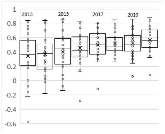
Figure 1.
Box-whisker summaries of normalized Refinitiv data for the DJIA data listed in Table S1.
Very few of the stocks have scaled ESG values that are negative, reflecting the fact that very few (and none for 2018 through 2020) stocks have a Refinitiv score below 50. The ESG scores of the lower rated companies improved fairly rapidly over the period 2013 through 2017. Adjusting the linear normalization to reflect a yearly change in the median ESG value (which might, for example, be interpreted as the appropriate percentile for separating “good” from “bad” ESG ratings) would introduce hidden variability into (1).
It is our perspective that there are (and, probably, need to be) inherent nonlinearities within an agency’s methodology for ESG scoring. This perspective is discussed further in Rachev et al. (2024, Appendix A), where possible monotonic transformations such as exponential or geometric, are suggested. Ultimately, they conclude that the choice of transformation should be based on an axiomatic approach to ESG investing. We amend this conclusion to suggest that, in practice, the transformation must depend on a precise analysis of the methodology used by any particular agency. Thus, addressing the normalization transformation of the ESG scores in further depth remains outside of the intended scope of this paper; we proceed with the linear transformation (2) to normalize the provided Refinitiv scores from to .
4. ESG-Valued Portfolio Optimization
We apply the ESG-valued return model (1) to portfolio optimization. We consider a quite general framework; at the end of day t an investor has to decide how to reallocate the value of a portfolio among a universe of I assets by selecting the fraction (the weight) to be invested in asset for the next day’s trading. The investor observes the series of previous asset returns and, based upon some discrete-state, parametric or non-parametric statistical model, obtains a series of S one-period-ahead returns . Under these assumptions, given the (column) vector of portfolio weights , (where denotes transpose) the simulated ESG-valued return of the portfolio between the close of trading on days t and is defined by the set of S scenarios16
where
We assign the weights by optimizing the trade-off between the risk and reward of the portfolio. The reward is usually measured by the expected value of the future ESG return , whereas there are many choices for the risk measure .17 Once the risk measure has been selected, the optimal long-only portfolio is obtained by solving the minimization problem,
subject to the constraints
where represents the risk-aversion attitude of the investor. The second constraint forces the portfolio turnover to be less than a prespecified value ; here, , are the previously optimized portfolio weights used during trading day t.
In a portfolio subject to actively managed stock selection, short selling generally reflects a belief that the stock price will decline. If stock selection is managed via algorithmic optimization, as performed here, a positive correlation (for example) between ESG score and financial return would lead optimally to short sales on low ESG/low expected return stocks. Since our model assumes no correlation between ESG scores, expected return and the risk measure, the short selling options become much richer. Would low ESG—high return sin stocks be a short-sell target? For high risk stocks, what combination of ESG scores and returns would be shorted? To skip this complex issue for now, we have imposed a long-only constraint in (6).
4.1. ESG-Efficient Frontier
We illustrate ESG-valued optimization by application to a specific portfolio consisting of 29 of the 30 stocks18 comprising the DJIA. We use the ESG scores in Table S1 provided by Refinitiv for each asset over the years 2013 through 2020. We employ the methodology discussed in Section 3.1 to obtain daily ESG scores.
To generate the ensemble of values in (4), we applied an ARMA()-GARCH(1,1) model (Ghalanos, 2024) to the set of historical returns . We fit the ARMA parameters and over the ranges , using the Bayesian information criterion. Separate fits were performed for each stock. For each asset, a GARCH(1,1) fit was then performed on the residuals of the best-fit ARMA model assuming that the innovations are normal inverse Gaussian (NIG; Barndorff-Nielsen, 1977, 1997). In the case in which the GARCH-NIG failed to converge, the autocorrelation , was computed to check for persistence. If no persistence was found, the GARCH(1,1) component was dropped in preference of a pure ARMA model.19 The resultant set of ARMA()-GARCH(1,1) innovations was then fit to a multidimensional NIG model (Weibel et al., 2013). From the parameterized, multidimensional NIG model, innovations were randomly generated. The generated innovations for asset i were then fed into the ARMA()-GARCH(1,1) fit to generate S sample returns for day for asset i. The use of ARMA-GARCH with an NIG distribution family for the innovations was motivated by its flexibility in modeling potentially different heavy-tailed behavior for each asset, while providing no-arbitrage option pricing (Chorro et al., 2010). Since NIG distributions are closed under affine transformations, the ESG-valued returns (4) remain within the same distribution class as the financial returns, preserving the semimartingale property.
Two choices were used for the risk metric in (5): mean-variance (MV) to capture central risk, and mean-CVaRβ (mCVaRβ) with percentile levels and to capture increasing tail risk. This latter choice aligns with modern market risk approaches for determining minimum capital requirements (Basel Committee on Bank Supervision, 2019). In addition, mCVaRβ has superior properties as a risk measure. As opposed to the Sharpe ratio (which lacks the property of monotonicity) used to define the tangent portfolio in MV optimization, the Sortino ratio used to define the tangent portfolio under mCVaRβ optimization is a coherent risk measure (Cheridito & Kromer, 2013).
Details on solving the minimization problem (5), (6) using each of these measures are provided in Appendix A. With denoting the vector of optimal weights, we can define the optimal portfolio return and ESG-valued return,
where are the realized asset returns on the close of trading day , from which the ESG-valued returns are computed using (4). The portfolio price is computed in the usual manner,
The ESG-valued numeraire for the portfolio is similarly defined as
We assign the initial value of this numeraire to be .
We emphasize that the numeraire is not a price in the sense that is. The ESG return (1) introduces a third dimension, ESG, to the portfolio optimization space, and represents the value of the portfolio as a cumulative combination of return and ESG values. We will refer to as the ESG-valued price or, for brevity, the ESG price.20 When the word “price” is used without the ESG qualifier, it shall refer to the value of . This usage is consistent with the distinction made earlier between “ESG-return” and “return”. When , ; any significant differences between and only occur for . Thus, the critical question as to whether a higher ESG price also corresponds to an improved financial price is one that can be examined naturally within our approach.
The normalized ESG score for the optimized portfolio is
As we have invoked a linear normalization , this is equivalent to
We illustrate the optimization procedure by solving for optimal weights for the date 30 December 2019 for our illustrative portfolio. We used an in-sample period of days and generated simulated returns. Optimizations were obtained using MV, mCVaR0.95 and mCVaR0.99 risk measures and for four choices of . For each , the efficient frontier was computed using the sequence of values {0, 0.01, 0.02, …, 0.99}.21 The efficient frontier can be examined either in the three-dimensional space or in . The efficient frontiers are plotted in space in Figure 2.
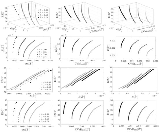
Figure 2.
ESG-valued return efficient frontiers (top) plotted in space and (following rows) in various projected planes. Left to right in each row: MV, mCVaR0.95 and mCVaR0.99 optimizations. Points on each curve represent equally spaced values of {0, 0.01, 0.02, …, 0.99}.
Also shown are the projections of these efficient frontiers onto the , , and planes.
Projection onto the plane corresponds to the usual risk-return view in modern portfolio theory. These projected curves are smoothly varying and concave, allowing for the solution of a well-defined tangent portfolio (see Section 6). For a fixed value of the risk-aversion parameter , the ESG risk decreases as the investor ESG affinity increases, while the ESG return increases with . When the risk measure is MV, as grows, increases more rapidly over small values of .
Projection onto the plane addresses the question of how the portfolio ESG score varies with expected ESG return. For each value of , the portfolio ESG score grows essentially linearly with for both MV and mCVaR risk measures. Also, for each risk measure and fixed value of , both and grow with . Again, when the risk measure is MV, as grows, increases more rapidly over small values of . Thus, for larger values of the ESG affinity , the portfolio ESG score and ESG return become more sensitive to changes in the risk-aversion parameter when the risk measure is MV (central risk) than when it is mCVaR (tail risk).
Finally, projection onto the plane addresses the question of how the portfolio ESG score varies with the ESG-risk measure. Reflecting the linear dependence observed in the () plane, the projections in the plane are qualitatively similar to those seen in the plane.
Figure 3 investigates the results in space, using the traditional financial risk and financial return axes.
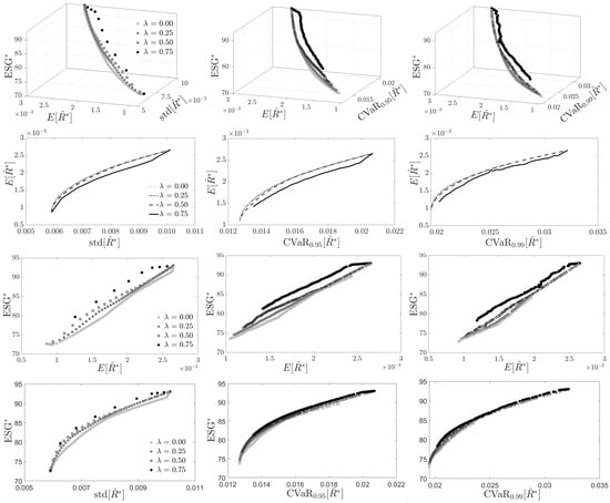
Figure 3.
ESG-valued return efficient frontiers (top) plotted in space and (following rows) in various projected planes. Left to right in each row: MV, mCVaR0.95 and mCVaR0.99 optimizations. Points on each curve represent equally spaced values of {0, 0.01, 0.02, …, 0.99}.
In parallel with Figure 2, it also displays the projections of the efficient frontiers onto the , and planes. Note that the efficient frontiers correspond to the traditional efficient frontier under which ESG scores are not considered. As , the efficient frontiers (and their plane projections) in Figure 3 are identical to the corresponding curves in Figure 2. In contrast to the efficient frontiers in Figure 2, which are approximately evenly spaced apart as varies over the set , the spacing of the efficient frontiers in Figure 3 indicate a non-linear dependence on .22
As shown in the projected plane (corresponding to the usual efficient frontiers in modern portfolio theory) the efficient frontiers lose their concave form when becomes sufficiently large. Consequently, a unique tangent portfolio cannot be guaranteed when working in space and must be defined in space. For either of the risk measures, there is little change in the efficient frontier in this projection until increases from 0.5 to 0.75. Again, for the MV risk measure at the larger values of ESG affinity, we see a rapid change in both ESG score and expected financial return over the low range of values of the risk aversion parameter .
In the projected plane, for fixed , the dependence between the portfolio ESG score and its expected financial return is approximately linear, though with less of a linear relationship than that displayed between and .
In the projected plane, there is only relatively minor separation of the efficient frontiers as changes, with the least separation occurring for the mCVaR0.99 risk measure. The results in the case of the MV risk measure are similar to the findings presented in the 12 July 2022 report by ISS LiquidMetrix.23 Figure 4 in that report demonstrates that the 33rd and 67th percentiles of the volatility (measured in terms of historical standard deviation) change relatively slowly as the ESG class ranking (an analog of our variable ) of an S&P 500 stock increases, with the exception that the change is slightly larger for the highest rank class considered.
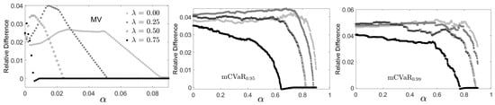
Figure 4.
Relative difference between the ESG score of the 30 December 2019 MV and MCVaR optimized portfolios computed using ESG scores released on 31 December 2019 (out-of-sample) compared with the computations obtained using ESG scores released on 31 December 2018 (in-sample). Note the truncated range of the axis for the MV optimized results.
An important question is “Which of the behaviors displayed in Figure 2 and Figure 3 are general to the model and which are data specific?” Some of these questions are immediately addressable. The increase of with follows from (4); increasing puts more weight on optimizing the ESG score of the portfolio. The observed increase of with follows from the same reasoning. As we hold ESG scores constant throughout a year’s time, increasing puts more weight on resulting in the observed decrease of . Under the optimization (5), (6), the efficient frontiers projected onto the plane will have the usual properties of an efficient frontier, specifically smoothness, concavity and efficiency relative to the individual assets comprising the portfolio. As demonstrated in Figure 3, smoothness and concavity does not necessarily hold for the projection of the efficient frontiers onto the plane.
For this portfolio and date, on the frontier, increases with increasing values of , the choice of more risky portfolios giving rise to a higher ESG score. This is not a general result as it depends on the distribution of returns estimated at the particular date. In Section S1, we show the efficient frontiers computed for 30 March 2020. For this date, on the efficient frontier the portfolio ESG score initially increases with , but then decreases as and risk continue to increase.
Since new ESG scores arrived on 31 December 2019, the choice of the optimization date of 30 December 2019 enabled a test of the stability of the optimization results by comparing the use of in-sample (released on 31 December 2018) versus out-of-sample (released on 31 December 2019) ESG scores. Figure 4 plots the relative difference24 between the ESG score of the optimal portfolio computed using individual asset ESG scores released on 31 December 2019 compared with the computations in Figure 2 and Figure 3 computed using the ESG data released on 31 December 2018.
In general, over all three risk measures, the relative difference does not exceed 5%, indicating a quite stable ESG portfolio value (at least for this date and these securities). The relative difference becomes zero as increases, approaching zero at successively smaller values of as increases. For the MV-optimized portfolios, the relative ESG difference rapidly disappears over the range . The sensitivity of the MV optimal solution to ESG score dramatically decreases for values as the optimized portfolios become extremely concentrated in very few securities. The relative difference persists longest under mCVaR0.99 optimization, staying roughly constant until .
While modern portfolio theory draws attention to the efficient frontier and the risk–reward plane, the fundamental optimized variable is the weight composition . In Figure 5 we depict the weight components along the efficient frontiers (i.e., as a function of ) of the mCVaR0.99 optimizations for each value of considered.
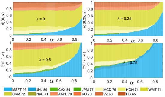
Figure 5.
Weight composition of the mCVaR0.99 optimal portfolios along each efficient frontier as a function . Each panel corresponds to a different choice of . The legend identifies each stock and the stock’s ESG score as assigned by Refinitiv on 31 December 2018.
Of the 29 stocks considered, only 13 contribute to the portfolio composition. As expected, when , these 13 are representative of the entire range of ESG scores. Interestingly, as increases, high ESG stocks from the remaining set of 26 do not begin to show up in the portfolio; rather, the portfolio weights concentrate on a smaller set of the representative 13. The concentration is not linear; the most rapid change in the composition of MSFT and JNJ (ESG scores of 93 and 89, respectively) occurs when changes from 0.5 to 0.75. In contrast, the weights of CVX and JPM (ESG scores of 84 and 77, respectively) do not increase with . Meanwhile, WMT having an intermediate ESG score of 74 continues to be strongly represented at while the weights of stocks with ESG scores of 70 and below are significantly decreased.
These observations of dependence of weight composition on hold qualitatively over most of the range of the risk-aversion parameter . Changes in weight composition occur most dramatically at the higher values of (acceptance of higher risk to gain ESG-valued return). When , the portfolio consists MSFT (ESG 93) and WMT (ESG 74) with small weights given to lower ESG valued stocks (KO, VZ, PG). When , the portfolio is comprised of two stocks, MSFT and MWT; and for , this portfolio is comprised solely of MSFT. Similar results (not shown) were obtained for the MV and mCVaR0.95 optimizations.
5. Performance over Time
We investigate the ESG-optimized investment results over time using the DJIA-derived portfolio of stocks of Section 4.1. We consider a daily investment horizon spanning the period 3 January 2017 through 30 December 2020. Using the procedure outlined in Section 4.1 involving one-day ahead forecasting based upon two years of previous returns, for each day t we computed an efficient frontier using the sequence of values for each value of , obtaining a set of optimal asset weights for each combination. We employed only the MV and mCVaR0.99 optimizations to examine central and tail behavior. Transaction costs were included in the evaluation by assuming a cost of two basis points for each buy and each sell order executed in rebalancing the portfolio. We imposed a daily turnover constraint of 0.4% ( in (4)) to approximate reasonable business practice. The results are compared to a benchmark consisting of the equally weighted, buy-and-hold portfolio (EWBH) of the same 29 DJIA stocks.25
The time series for both the price and ESG score for the point of the efficient frontiers of the mCVaR0.99 optimized portfolios are shown in Figure 6. The values for the benchmark portfolio, EWBH, are also shown. As previously noted, the optimized portfolios were computed with a daily turnover constraint of 0.4%. For discussion purposes, these optimizations were recomputed with no turnover constraint. The resultant time series for the unconstrained optimizations are also plotted in Figure 6. With no turnover constraints, the ESG-optimized () portfolios outperform the benchmark, both in cumulative price and ESG score. With a realistic daily turnover constraint of 0.4% to control transaction costs, the price of the EWBH benchmark outperforms that of the optimized portfolios until the COVID-19 pandemic. Post crash, the portfolio exhibits strong price recovery while the portfolio displays recovery competitive with that of the benchmark. Each turnover-unconstrained portfolio rapidly establishes a separate ESG level (around which it displays variance). Under the turnover constraint, the portfolio ESG scores climb to their separate levels more slowly, but with much less variance. The noticeable discontinuity in portfolio ESG scores on 1 January 2020 arises from rather large changes in the ESG ratings of a number of these companies in the 31 December 2019 data release compared to that of 31 December 2018. (See Table S1).
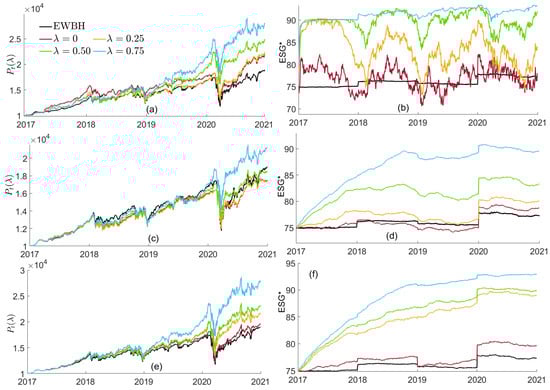
Figure 6.
(a–d) Time series over the period 3 January 2017 through 30 December 2020 of the price and the ESG score for efficient frontier portfolios obtained from the mCVaR0.99 optimization with (a,b) no and (c,d) 0.4% daily turnover restriction. Plots (e,f) are for the tangent portfolios with 0.4% daily turnover restriction. In each, a comparison is made against the equi-weighted portfolio EWBH. The initial price was arbitrarily set to 10,000.
The efficient frontier portfolios were evaluated using standard performance measures: total return (Tot Rtn), annualized return (Ann Rtn), average turnover (AvgTO), expected tail loss (ETL95) and expected tail return (ETR95), both at 95% percentile levels, and maximum drawdown (MDD).26 ETR95 is the reward counterpart of ETL95, measuring the average value of those returns above the 0.95 percentile. MDD is defined as the maximum drop of portfolio returns over all time intervals that can be formed as a partition of the investment period (Cheklov et al., 2005). As performance measures, we also considered the average ESG score of a portfolio over the time period, as well as its standard deviation. Tables S2 and S3 present time-averaged values for these summary performance measures for select ()-efficient frontier portfolios for both mCVaR0.99 and MV optimizations.
The total and annualized returns of the optimized portfolios are generally superior to that of the benchmark for values of for mCVaR0.99 and for MV optimizations. For fixed , as increases, AvgTO tends to fall below the daily constraint value of 0.4%. For fixed , AvgTO decreases with . This effect is of particular importance under MV optimization, which can suffer from solution instability and high turnover rates, which, in turn, can downgrade financial performance (Clarke et al., 2002; Kirby & Ostdiek, 2012; Michaud, 1989). For mCVaR0.99, except for the largest values of and , the magnitudes of ETL95 and ETR95 are less than that of the EWBH benchmark. For MV, these magnitudes generally exceed that of the benchmark. In the optimized portfolios, ETL95 always exceeds ETR95 in magnitude, with the suggestion that, for MV optimization, at large values of the magnitude difference decreases as increases. All optimal portfolios have lower MDD than the benchmark. For optimization under mCVaR0.99, the MDD decreases with for each fixed value of . Average ESG scores for the optimized portfolios virtually always exceed that of the benchmark. Under mCVaR0.99 optimization, the standard deviation of the ESG score is generally smaller than that of the benchmark; for MV optimization, the reverse is true.
We computed moment values for the distribution of the financial returns for the same () selection of efficient frontier portfolios, as in Tables S2 and S3. Specifically, we consider the mean, median, standard deviation (Std), skewness (Skew) and excess kurtosis (ExKurt). Table S4 summarizes these values for both optimizations. For each fixed value of , mean, median returns and the Std increase with , much more so under MV optimization. Skewness and ExKurt decrease as increases.
5.1. ESG-Valued Reward–Risk Ratios
A common approach to evaluate the performance of an investment strategy is to use one or more reward–risk ratios (RRRs) to quantify the trade-off between expected reward and the risk associated with the strategy. There is an extensive list of such ratios, though not all of them possess the properties of a coherent risk measure; see Cheridito and Kromer (2013) for a complete overview of RRRs and an analysis of their properties. For instance, the extensively used Sharpe ratio does not satisfy the monotonicity property. The development of ESG-valued RRRs involves questions concerning the desired properties that the measures should possess; for example, the coherent risk measure properties may comprise a necessary but not a sufficient set of properties for ESG-valued RRRs. Such questions are outside the scope of this paper; we illustrate here a “straightforward” strategy for developing ESG-valued RRRs.
For any choice of an RRR, replace the portfolio return with the ESG-valued return . For illustration, we consider the stable tail ESG return (STAR) ratio (Martin et al., 2003),
where is a risk-free rate appropriate for day t and is the expected tail loss at percentile level .27 The ESG-valued STAR ratio is then28
The ESG-valued STAR ratio satisfies all four properties of a coherent risk measure. As the STAR ratio will vary along the efficient frontier (i.e., with ) and from frontier to frontier (i.e., with ), in Figure 7 we summarize the behavior of the STAR ratio as the surface STAR() for the mCVaR0.99 optimization.
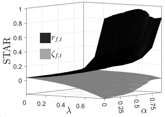
As only four values for were computed while the grid is much finer, the smoothly interpolated surface appears coarser in the direction. The surface shows a generally convex relationship between the ESG-valued STAR ratio and and , although variation with is smaller. The “kink” that appears in the efficient frontier produces the non-convexity observed in the surface.
A more consistent definition of the ESG-valued STAR ratio would also replace with an ESG-valued risk-free rate, such as that developed in (13). Figure 7 also shows the surface STAR() for the mCVaR0.99 optimization using the formulation
with defined in (13). Because the risk-free rate has no dependence, as increases the behavior of the STAR ratio is effectively that of , which increases with . In contrast, the risk-free rate has strong dependence, especially since this risk-free rate is assigned an ESG score of 100, larger that that of any asset in the optimized portfolio and, consequently, larger than that of the portfolio. As a result, for large , the term becomes the dominating factor in the numerator and denominator of (15). Apparently this effect exists even for small, positive values of , resulting in a monotonic decrease in the STAR ratio as increases. In contrast to the surface, which shows no strong dependence, as increases, the dependence of the surface becomes more pronounced and the STAR ratio decreases with a decrease in (more risk-averse optimization producing smaller STAR ratios). The STAR ratio becomes negative under these conditions.
We computed the performance of the DJIA-derived portfolios relative to the ESG-valued versions of five popular RRRs: the Sharpe (SR), Sortino, STAR, Rachev and Gini ratios (Cheridito & Kromer, 2013).29 These values are summarized in Table S5. The optimized portfolios generally produce superior ESG-vAlued RRR values compared to the benchmark over all ranges of and . For and , the ESG RRRs for MV generally outperform those for mCVaR0.99.
When , the choice of does not significantly alter the performance of the optimal portfolios as the investor is only concerned with the risk of the investment, which is unaffected by the ESG score.
6. ESG-Valued Tangent Portfolios
The efficient frontiers in the plane (see Figure 2) can be used to identify the ESG-valued tangent portfolio and a capital market line.30 Determining the tangent portfolio for each ESG-valued efficient frontier in this space requires identification of an appropriate risk-free rate process . The appropriate risk-free rate to be used should also be ESG-valued, as in (1). This raises the issue of assigning an ESG score to a fixed-income security, in particular to any government bond.31 As a first attempt to address this, we proceeded as follows. We used the yield on the 10-year U.S. treasury bond (appropriately scaled to daily rates) and assigned the government bond a maximum ESG score of 100.32 The motivation behind this choice is that the risk-free rate is not among the set of choices available to the investor; any other ESG value for the risk-free rate will be more arbitrary than simply assigning the maximum value. From (1), the appropriate ESG-valued riskless rate is then
Consistent with previous nomenclature, the phrases “ESG-valued riskless rate” or “ESG riskless rate” shall refer to while “riskless rate” with no ESG adjective shall refer to . The ESG-valued tangent portfolio for date t will be uniquely determine by the straight line from the point which is tangent to the -specified ESG-valued efficient frontier.
Using (16), the ESG-valued tangent portfolio can be identified on any efficient frontier parameterized by ().33 These ESG-valued tangent portfolios were identified for the 0.4% daily turnover constrained portfolios computed in Section 5. Figure 6e,f show the price performance , as well as the ESG scores for the tangent portfolios computed with mCVaR0.99 optimization. For , the price performance of these turnover-constrained tangent portfolios is competitive with that obtained by the turnover-unconstrained, efficient frontier portfolios (compare Figure 6a,e). Allowing for the initial transient behavior due to the turnover constraint, for the ESG scores for the turnover-constrained tangent portfolios are superior to those for the turnover unconstrained, efficient frontier portfolios (compare Figure 6b,f).
The ESG price time series are displayed in Figure 8 for these mCVaR0.99 optimized tangent portfolios. time-series are also shown for the EWBH benchmark as well as for an ESG-valued DJIA index.34 Note the close agreement between ESG prices for the EWBH- and ESG-valued index; both portfolios are comprised of the same stocks, with different weights applied. The differences between ESG prices for the ESG-valued tangent portfolio and the ESG-valued index are also plotted in Figure 8. As increases, the differences between the ESG prices of the optimized portfolio and those of the benchmarks (Figure 8e) grow more rapidly than the corresponding differences between optimized portfolio and benchmark price series. (The latter differences can be determined from Figure 6e).
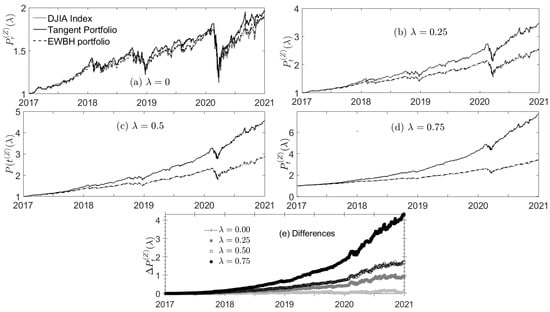
Figure 8.
(a–d) ESG prices (with ) obtained for the tangent portfolios under mCVaR0.99 optimization, compared with the corresponding time series for the EWBH strategy and the ESG-valued DJIA index. (e) Difference between the values for the tangent portfolios and the ESG-valued DJIA index.
Table S6 provides the performance, moment and RRR measures for these four tangent portfolios. At the higher values of , the tangent portfolios outperform the benchmark. Compared to the benchmark, total (and hence annualized) return almost doubles for the tangent portfolio as increases. With the exception of one Gini value, the value for every RRR considered is better than the benchmark as increases. Trivially, the tangent portfolio average ESG score improves with . (The standard deviation of ESG decreases because more weight is given to the ESG score, which remains constant over each year.) The average turnover considerably decreases as increases.
7. ESG-Valued Option Pricing
We consider the effect of ESG-valued returns on option pricing. Paralleling our established notation, we shall refer to the valuations given to options using ESG-valued returns as “ESG-valued option prices” or simply “ESG option prices” to distinguish from the valuation of options based on traditional financial returns. When , ESG option prices are equivalent to traditional option prices. For a given date t, using the discrete methodology outlined in Appendix B, we computed European contingency claim ESG option prices for a sequence of expiration dates , and strike values35 using an ESG-valued tangent portfolio as the underlying. We chose the date t = 30 December 2019 corresponding to the efficient frontiers discussed in Section 4.1 and Section 6. ESG option prices were computed for each tangent portfolio. The same methodology was employed to obtain ESG option prices for 30 December 2019 using the ESG-valued DJIA index as the underlying. We are interested in the difference between ESG option prices based upon the ESG DJIA index and the tangent portfolios.
Call and put ESG option prices were expressed as functions of T and “ESG-moneyness” . We considered ESG-moneyness values in the range and maturity times days. Comparisons of the call and put ESG price surfaces based on the ESG-valued DJIA index and on the mCVaR0.99 optimized tangent portfolio for selected values of are given in Figure 9.
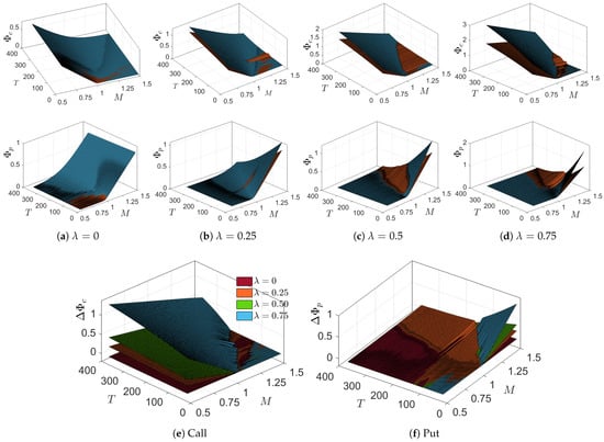
Figure 9.
(a–d) Call (top) and put (bottom) ESG option prices for select choices of . The orange surfaces correspond to ESG option prices for the ESG-valued DJIA index; blue surfaces represent ESG option prices for the mCVaR0.99 tangent portfolios. (e,f) The differences in call and put ESG option prices between the ESG-valued DJIA index and the mCVaR0.99 tangent portfolios.
The respective call and put ESG option price differences, and , between the tangent portfolios and the DJIA index are also given in Figure 9.
When , call and put ESG option prices (and hence, call and put option prices) written on the index and the mCVaR0.99 tangent portfolio are practically equal. The difference increases with , especially as strike values move further into-the-money. By construction, ESG-valued tangent portfolios have a higher ESG score, which in turn implies a positive shift in their aggregate value, creating higher call and put ESG option prices. The effect of a positive on call and put ESG option prices is different as a function of time to maturity; at constant in-the-money values of K, call ESG option prices increase with T while put ESG option prices decrease.
Figure 10 compares implied volatility (IV) surfaces, computed by fitting to the Black–Scholes model, for call options based on the DJIA index and the mCVaR0.99-optimized tangent portfolios. For and in-the-money K values, the IV surface of the DJIA index is above that of the tangent portfolio for short maturity times. For longer maturity dates it drops below. As increases, the two IV surfaces move upwards (overall volatility increases); the difference between the surfaces decreases; and the volatility “smirk” becomes steeper.
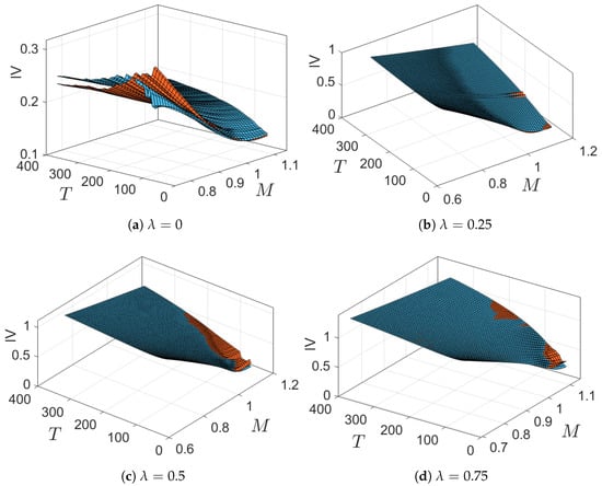
Figure 10.
Implied volatility (IV) surfaces computed from the (orange surfaces) ESG-valued DJIA ESG option prices and (blue surfaces) the tangent portfolios corresponding to the selected choices for .
8. ESG-Valued Shadow Riskless Rate
The existence of a risk-free rate in the economy is a common and implicit assumption of modern financial theory. However, the situation in which the risk-free rate is not available for a market has been also considered. The seminal work is that of Black (1972), who proposed a CAPM model without assuming the existence of a riskless rate. Black (1995) later introduced a “shadow real rate” as an option on fixed-income derivatives. More recently, a different approach was introduced by Rachev et al. (2017), in which a shadow riskless rate is defined as a perpetual option on the set of risky securities selected as the investment universe. Rachev at al. computed analytic formulas for the shadow riskless rate under different models of the stochastic process driving the market uncertainty. The simplest case, where diffusion is driven by Brownian motions, is summarized in Appendix C.
We analyze the effect of ESG-valued returns on the shadow riskless rate (SRR) derived in (A15). For an investment universe defined by the 29 stocks comprising our ESG-valued DJIA index. For each trading date in the period from 3 January 2017 through 31 December 2020, using two-year moving windows, we estimated the vector of mean values of, and the variance-covariance matrix Σ for the 29 stock returns. The asset (row) entries in Σ were sorted in order of decreasing variance value. The elements required in (A15) were obtained from the upper triangular matrix obtained from the Cholesky decomposition . To eliminate one dimension and obtain 28 Brownian motions, the last column of was replaced with a linear combination of its last two columns.36
Using the values , the SRR computations were performed on the ESG-valued DJIA index.37 The time series for these four SRRs are presented in Figure 11. The SRR levels show separation in rough proportion to the value of ; however, this proportion is affected by each year-end readjustment of ESG values. The separation between SRR curves appears to be roughly constant for the calendar years 2017 and 2019. Over 2018, the separations between the curves narrow. The COVID-19 crash in 2020 initially removed differences between SRR curves, after which they again began to separate.
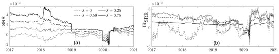
Figure 11.
Time series from 3 January 2017 through 31 December 2020 for select values of of (a) the SRR computed from ESG-valued returns on a universe of 29 DJIA assets and (b) the information ratio of the SRR.
We define the standard deviation of the price deflator process by . This enables the definition of the SRR information ratio, . The four time series for IRSRR are also plotted in Figure 11. For each time series, the average and standard deviation values of IRSRR can be computed. The behaviors of and for { 0, 0.01, 0.02, …, 0.89, 0.9} are presented in Figure 12. The value of initially grows with , reaching a maximum time-averaged IRSRR value at , after which the averaged SRR information ratio decreases. The standard deviation decreases with ; for , the decrease is linear. These results quantify the nonlinear impact of on the shadow riskless rate.
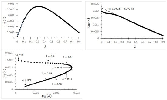
Figure 12.
The curves , and the parametric curve . The dashed line is a linear fit.
9. Variation in Agency-Provided ESG Scores
As noted in Section 2, the definition of methodologies and the consequent creation of databases related to ESG scores has experienced huge growth in the last ten years, resulting in a wide set of options in the choice of rating agency. Although it is not our intention to address this issue in depth, as has been extensively explored in the literature cited, we provide some insight on its impact on our ESG valuation framework by considering scores from a second provider. In Sections S3 through S9, we have repeated the computational results presented in this article using ESG scores provided by RobecoSAM. Despite the general disagreement of ESG scores between these two providers, we have observed that optimal portfolio performances, and hence efficient frontiers, on the DJIA universe of assets present relative stable results between the two scoring systems. This in turn implies stable results for the option pricing example in Section 7. However, optimized portfolio compositions can change considerably when computed with RobecoSAM scores. This in turn is reflected in the shadow riskless rate implicit in the market, even if computed under Gaussian hypotheses, exhibiting wide variation in the SRR depending on the score system used. These results confirm the need for a stronger effort toward a convergence in agency methodologies used to asses ESG scores.
10. Discussion
In response to environmental challenges and investor, societal and governmental pressure, ESG ratings are assuming an important role in financial markets. Thus motivated, we have introduced a consistent ESG-valued framework for the inclusion of ESG ratings into dynamic pricing theory. There are two fundamental parameters in the framework; in addition to the traditional financial risk aversion parameter , we introduce the ESG affinity parameter . When , our pricing framework reduces to traditional financial-risk versus financial-reward valuation. As increases, the framework places increased emphasis on the impact of ESG ratings on valuation. Thus, our results are presented in terms of comparisons of valuations for compared with . In this work, we applied the ESG-valued framework to portfolio optimization, risk measures, option pricing and the concept of shadow riskless rates. Although the ESG-valued return (1) is linearly dependent on ESG scores through , other nonlinearities in portfolio and option valuation ultimately result in non-linear dependence on .
The philosophy incorporated in our framework is that socially responsible investing places a value on an investment portfolio that is competitive with (or “additional to”) financial return. The market’s emphasis on that value is adjusted through the ESG affinity parameter. As a consequence, our framework requires valuations (e.g., ESG returns, ESG prices, ESG option prices, ESG riskless rates) in terms of an ESG-valued numeraire (the ESG price) which reduces to a standard financial numeraire when . Standardization of such an ESG numeraire will become necessary if ESG valuation is to be adopted. This would require, among other things, the development of market indices expressed in terms of a standard ESG numeraire. Introduction of this ESG-valued numeraire has an additional positive benefit. A company whose ESG score is near or at the upper bound has no incentive to improve. Company X with a maximum ESG score of 100 in year t and again in year experiences a “return” of zero on its ESG score. However, said company’s ESG price can grow from year t to .
If adopted, a framework such as that developed here will require consideration of a myriad of issues, some of which are being pursued as described in Section 2; others arise from considerations encountered while implementing the framework. In our view, one of the most important limitations is the deterministic nature of the ESG rankings employed here. Given the current and foreseeable variation in ESG rating systems and methodologies, our framework accommodates (and in fact argues in favor of) ESG ratings as random variables whose stochastic properties reflect these variations. Evaluation of these properties will become more definitive once ESG ratings are updated at higher frequencies. Ideally, company-specific ESG ratings would adapt on a time scale intrinsic with the company’s activity.
Our work reveals that the adoption of an ESG-valuation framework will require resolution of critical research issues. (i) Our model requires that ESG ratings be rescaled to be comparable to financial returns, which requires scaling to a bounded interval with , . This requires the identification of a threshold ESG value satisfying , which effectively separates “good” ESG ratings from “bad” ESG ratings. (ii) Traditional financial-reward: financial-risk metrics must be modified to incorporate ESG ratings, thus becoming ESG-valued-reward:ESG-valued-risk metrics.
This raises the research question of “coherence”, the necessary set of properties that such adjusted metrics should satisfy. (iii) As excess return is often measured relative to a government set risk-free rate, the concept of applying ESG ratings to governments and government-issued bonds becomes a required research focus. (iv) The option pricing model explored here is based upon a discretization of a continuum model which captures limited information (specifically, only the standard deviation of the financial returns of the underlying). Thus, another research avenue is the application of this ESG-valued framework to option valuation models that are capable of capturing more of the microstructure of the underlying asset price (and, when it becomes available, that of its ESG ratings).
To conclude this discussion, we note that our paper does not address the question “Why does ESG generate the financial returns that it does?” Given the current state of the industry—with no agreed upon criteria and methodology— the answer to that question remains highly dependent on the rating agency chosen. What our work does provide is a dynamic asset pricing model based upon assumptions we contend are reasonable, that can provide the financial tools (optimization, risk measures, risk-free rates, option pricing) that will work with any choice of rating agency. Given the current variation in criteria and methodologies, we suggest that the answer to the “Why?” question is best addressed by replacing the (single agency) ESG score in our analysis by an ESG information ratio—specifically a mean ESG score (over all providers) divided by the standard deviation of their scores. This treats the ESG score as a random process (a Lévy process perhaps?), which we believe is the appropriate model.
Supplementary Materials
The Supplementary Material referenced in this article by Supplementary Sections S1–S9, Figures S1–S11 and Tables S1–S13 can be downloaded at https://www.mdpi.com/article/10.3390/jrfm18030153/s1. Figure S1: Refinitiv-based ESG-valued return efficient frontiers for 03/30/2020; Figure S2: Box-whisker summaries of normalized RobecoSAM data for the DJIA data listed in Table S7; Figure S3: Normalized ESG ratings from Refinitiv and RobecoSAM for 2016 and 2020; Figure S4: RobecoSAM-based ESG-valued return efficient frontiers for 12/30/2019; Figure S5: Variation of the weight composition along each efficient frontier for the MCVaR0.99 optimal portfolios; Figure S6: RobecoSAM-based ESG prices, , obtained for tangent portfolios under mCVaR0.99 optimization; Figure S7: ESG values obtained by mCVaR0.99 optimized tangent portfolios and the EWBH benchmark under Refinitiv and RobecoSAM data; Figure S8: Panels (a) to (d): (top) call and (bottom) put option prices for select choices of . Panels (e) and (f). The difference in call and put option prices between the ESG-valued DJIA index and the MCV tangent portfolios; Figure S9: Implied volatility surfaces computed from the ESG-valued DJIA option prices and the tangent portfolios; Figure S10: Time series from 01/03/2017 through 12/31/2020 of (a) the SRR computed from ESG-valued returns on a universe of 29 DFJIA assets and (b) the information ratio of the SRR; Figure S11: The curves , and the parametric curve . Table S1: Refinitiv ESG scores for the DJIA index components; Table S2: Performance measure values for the mCVaR0.99 optimization obtained for the period 01/03/2017 through 12/30/2020 for select efficient frontier portfolios; Table S3: Performance measure values for the MV optimization obtained for the period 01/03/2017 through 12/30/2020 for select efficient frontier portfolios; Table S4: Moment values obtained for the return distributions over the period 01/03/2017 through 12/30/2020 for select efficient frontier portfolios optimized under mCVaR0.99 and MV; Table S5: ESG-valued reward-risk ratio values obtained for the period 01/03/2017 through 12/30/2020 for select efficient frontier portfolios optimized under mCVaR0.99 and MV; Table S6: Performance measures, moment values and ESG-valued reward-risk ratios obtained for the tangent portfolios under mCVaR0.99 and MV optimization over the period 01/03/2017 to 12/30/2020; Table S7: RobecoSAM ESG scores for the DJIA Index components; Table S8: Rank correlation measures between Refinitiv and RobecoSAM ESG ratings released in 2016 and 2020; Table S9: Performance measure values for the period 01/03/2017 through 12/30/2020 for select efficient frontier portfolios optimized under MCVaR0.99 using RobecoSAM data; Table S10: Performance measure values for the period 01/03/2017 through 12/30/2020 for select efficient frontier portfolios optimized under MV using RobecoSAM data; Table S11: Moment values for the return distributions obtained for the period 01/03/2017 through 12/30/2020 for select efficient frontier portfolios optimized under MCVaR0.99 and MV; Table S12: ESG-valued reward-risk ratio values obtained for the period 01/03/2017 through 12/30/2020 for select efficient frontier portfolios optimized under MCVaR0.99 and MV; Table S13: Performance measures, return moment values and ESG-valued reward-risk ratio results obtained for the tangent portfolios under mCVaR0.99 and MV optimization during the period 01/03/2017 to 12/30/2020.
Author Contributions
Conceptualization, S.T.R. and S.M.; methodology, D.L., W.B.L., S.M. and S.T.R.; software, D.L. and W.B.L.; validation, D.L. and W.B.L.; formal analysis, D.L., W.B.L., S.M. and S.T.R.; investigation, D.L. and W.B.L.; data curation, D.L.; writing—original draft preparation, D.L.; writing—review and editing, W.B.L.; visualization, D.L. and W.B.L.; supervision, S.T.R. All authors have read and agreed to the published version of the manuscript.
Funding
This research received no external funding.
Institutional Review Board Statement
Not applicable.
Informed Consent Statement
Not applicable.
Data Availability Statement
The data that support the findings of this study are available as follows. Refinitiv ESG rating data provided under license with Refinitiv. S&P Global RobecoSAM ESG ratings data provided through Bloomberg Professional Services and used under license. Stock price data provided through Bloomberg Professional Services and used under license. Ten-year treasury yield curve rates openly available at https://www.treasury.gov.
Conflicts of Interest
Author Stefan Mittnik was employed by the company Scalable Capital. The remaining authors declare that the research was conducted in the absence of any commercial or financial relationships that could be construed as a potential conflict of interest.
Appendix A. MV and mCVaRβ ESG-Valued Optimization
Extension of MV and mCVaRβ optimization to ESG-valued returns is straightforward. Consider a universe of I assets and the corresponding series of simulated ESG-valued returns ; ; . For MV optimization, let (with transpose denoted by ) denote the vector of the sample means and the corresponding variance-covariance matrix computed from this sample of ESG returns. Let , denote the portfolio weights. The ESG-valued, MV optimized, weight vector is obtained as the solution of the quadratic programming problem (Black, 1995; Markowitz, 1952, 1956).
subject to the constraints38
for a particular choice of and , where is the risk-aversion parameter, and is the ESG affinity parameter.
The ESG-valued, mCVaRβ-optimized, weight vector is obtained from the minimization (Rockafellar & Uryasev, 2000)
where
subject to
for a particular choice of and . In (A3), . We use 0.95 and 0.99 as the values for the percentile . Equations (A3)–(A5) can be reduced to a linear problem (Rockafellar & Uryasev, 2000).
Appendix B. ESG-Valued Option Pricing: Discrete Model
Consider the problem of valuing a European contingent claim on the underlying security on day t having strike value K and maturity date . We utilize the following discrete option pricing approach. Following the procedure in Section 4.1, we fit an ARMA()-GARCH(1,1) model to a two-year window of historical returns of , assuming that the innovations are distributed according to an NIG distribution. From the NIG fit, we randomly generate a set of of innovations, which, using the fitted ARMA-GARCH parameters, are converted into a return trajectory . We generate an ensemble of such return trajectories, . Using the ESG score for day t, from (1) each trajectory can then be converted to a trajectory of ESG-valued returns and consequently a set of ESG-valued price trajectories .39
We compute an ESG-valued price for call and put options in the standard way; the contract value is given by the discounted expected value of the contract pay-off, conditioned to a filtration , where the conditional expectation is with respect to a risk-neutral measure (Delbaen & Schachermayer, 1994), which discounts expected values at the ESG-valued risk-free rate defined in (13),
Given the risk neutral probability measure , European call (c) and put (p) ESG-valued option prices on the underlying can be computed as
In the discrete setting of this paper,
and the option valuation problem is reduced to identifying through the coefficients . We solve for these coefficients by minimizing the Kullback–Leibler divergence between and the natural world probability (Avellaneda et al., 2001). This involves solving the convex problem
subject to the constraints
In (A8), is the probability of trajectory s under . As each trajectory is equally likely, . Option values are then computed from the discrete version of (A7)
Appendix C. Shadow Riskless Rate
Consider a set of N risky securities whose prices ; are driven by Brownian motions40 . Thus,
To eliminate arbitrage opportunities in the market defined by (A13), we search for the unique state-price deflator
such that the discounted prices , are martingales. It is easy to show41 that this requirement is equivalent to solving the linear system
for . Following the treatment in Duffie (2001, Chapter 6D), the risk premium for each security is
where is the short-term shadow riskless rate observed in the market.
Notes
| 1 | Extensive literature reviews, such as those conducted by Friede et al. (2015) and Brooks and Oikonomou (2018), have revealed less-than-conclusive results regarding the strength of correlation between ESG scores and financial performance. |
| 2 | “It is also possible that Refinitiv ESG adjusted the methodology to take into account certain factors that happen to be correlated with firms’ stock price performance.”, Berg et al. (2021). |
| 3 | In the notation of Pástor et al., their ESG-valued return for investor i is expressed as , where is (a vector of) the excess financial returns for the assets under consideration, is the risk aversion coefficient for investor i, g is a (vector of) the “greeness” of each asset and is the “ESG taste”. Unlike our model, there is no constraint between the financial and ESG contributions to their return. |
| 4 | Due to the non-Gaussian nature of our portfolio optimization, we hesitate to postulate a capital asset pricing model based upon this capital market line. |
| 5 | In fact, their optimization can only depend on the ratios of two of these parameters relative to the third. |
| 6 | The determination of the resultant equilibrium model will not be straightforward, given the rich one-step ahead predictive environment involving ARMA-GARCH with NIG returns used in our portfolio optimization model. |
| 7 | Sections S1–S9, Tables S1–S13, and Figures S1–S11 refer to the Supplementary Material supplied as an online resource for this paper. |
| 8 | e.g., ESG Funds Resist Worst of Downturn But Investors Are Spooked (Bloomberg, 18 June 2022), https://www.bloomberg.com/news/articles/2022-06-18/esg-funds-are-losing-less-in-the-market-slump-so-far (accessed on 14 July 2022); ESG Backlash Has Fund Clients Demanding Proof It Works (Bloomberg, 31 May 2022), https://www.bloomberg.com/news/articles/2022-05-31/esg-fund-clients-demand-proof-strategy-works-amid-backlash (accessed on 14 July 2022); Sustainable Investing Failed Its First Big Test. A Reckoning Is Coming. (Barrons, 17 April 2022), |
| 9 | ESG Can’t Square with Fiduciary Duty. (Wall Street Journal, 7 July 2022), |
| 10 | We develop our formalism for daily trading. |
| 11 | This normalization is discussed in Section 3.1. |
| 12 | We note that ESG ratings are currently effectively updated by most rating agencies once a year. |
| 13 | Some literature has focused on the higher returns provided by portfolios based on certain ESG criteria. Pedersen et al. (2021) found that governance factors are more linked to financial performance than those related to environmental impact. |
| 14 | Although some providers distribute monthly scores, these data are usually expensive and are not provided on a regular basis. |
| 15 | Environmental, Social and Governance Scores from Refinitiv; accessed on 22 February 2021. |
| 16 | Equation (3) assumes the difference between daily log-return values and arithmetic return values is negligibly small. We continue this assumption throughout the paper. |
| 17 | Artzner et al. (1999) proposed an axiomatic approach to define the minimum set of properties that should satisfy to be a coherent measure of risk. Frittelli and Rosazza Gianin (2002) have specified requirements to define a convex risk measure. |
| 18 | Due to its shorter span of existence, stock from DOW Inc is not included in the portfolio. |
| 19 | Persistence was found to be both stock and time dependent; even for the same stock, the presence of persistence could change over time. |
| 20 | Settling on a nomenclature for for this article has not been easy. The phrase “ESG-valued numeraire” is awkward. The shorter “ESG value” leads to confusion between values of and values of ESG score. The phrase “ESG-valued price” or “ESG price” runs the risk of continuing to blur the distinction between and . Finding nothing better, we run that risk and will refer to as the ESG-valued price (ESG price for brevity). |
| 21 | For this portfolio, there is essentially no change in the optimized solutions over the range . |
| 22 | As a consequence of the non-linear spacing of the efficient frontiers, the curves in Figure 3d–f have been delineated through solid lines rather than points in order to be able to differentiate those corresponding to smaller values of . |
| 23 | Do ESG Ratings Impact Stock Price Volatility?, ISS LiquidMetrix report, 12 July 2022. https://www.issgovernance.com/library/do-esg-ratings-impact-stock-price-volatility/ (accessed on 14 July 2022). |
| 24 | The relative difference in the portfolio ESG score is defined in the usual manner as (ESG(out-of-sample) − ESG(in-sample))/ESG(in-sample). |
| 25 | With reference to Equations (7) and (8), the EWBH portfolio is defined as follows. ; the stock for Dow Inc. remains excluded. No scenario sets are generated; no optimization is performed. At , . For , the number of shares of each stock remains fixed at ; thus , where is the price of the asset at the close of trading day t. |
| 26 | Tot Rtn, Ann Rtn, ETL95, ETR95 and MDD are all computed on the financial returns. |
| 27 | Also known as conditional value-at-risk or expected shortfall. |
| 28 | To compute the STAR ratio, we used the 10-year U.S. treasury yield rate to determine daily values for . Computation of the expectation and ETL in the STAR ratio is performed over the ensemble of ESG-valued returns generated for day based upon the information available at day t. |
| 29 | Here we define the Sharpe, Sortino and STAR ratios using only the portfolio returns and not the excess returns relative to a benchmark. |
| 30 | While this approach can be used to formulate an ESG-valued capital asset pricing model and the two-fund separation theorem (Tobin, 1958), as noted in the introduction we prefer to derive the equilibrium formulation from this model based upon firmer principles. |
| 31 | The analysis of ESG factors associated with a fixed income security, especially one issued by a government entity, involves dealing with complex methodological and technical implications (Badía et al., 2019; Inderst & Stewart, 2018). |
| 32 | Another possibility is to use an ESG score for the appropriate country for a government bond. Some agencies are beginning to provide such scores, though not necessarily in the same scale used for companies. |
| 33 | It is critical to emphasize that the tangent portfolios are identified using the efficient frontiers computed in space and not in space. The optimization is performed in the former space, not the latter. As can be seen by comparing Figure 2 and Figure 3, convexity of the efficient frontiers can only be guaranteed in the former space. |
| 34 | With reference to Equations (7) and (8), the DJIA index is defined as follows: . No scenario sets are generated; where is the DJIA published weight for component i and is the published weight for Dow Inc., which is excluded from our benchmark index. We utilized the published DJIA weights applicable to 30/12/2020 in composing our index. |
| 35 | For , strike values in this ESG formulation are not traditional strike prices. |
| 36 | There is currently no theory governing identification of the standard deviation parameters from the elements of the variance-covariance matrix of asset returns. The Cholesky decomposition approach used here is ad hoc. |
| 37 | We perform the SRR computations on the DJIA index rather than the optimized portfolios because the Dow Index is conventionally recognized as an indicator of the general health of the US stock market (though there are valid arguments against this). |
| 38 | As noted in Section 4, we consider long-only portfolio optimization. |
| 39 | For the computations in Section 6, we used , . |
| 40 | More complex pricing models have been considered (Rachev et al., 2017); here, we employ the basic Brownian motion model. |
| 41 | This follows directly from Itô’s formula. |
References
- Abate, G., Basile, I., & Ferrari, P. (2021). The level of sustainability and mutual fund performance in Europe: An empirical analysis using ESG ratings. Corporate Social Responsibility and Environmental Management, 28(5), 1446–1455. [Google Scholar] [CrossRef]
- Amel-Zadeh, A., & Serafeim, G. (2018). Why and how investors use ESG information: Evidence from a global survey. Financial Analysts Journal, 74(3), 87–103. [Google Scholar] [CrossRef]
- Artzner, P., Delbaen, F., Eber, J.-M., & Heath, D. (1999). Coherent measures of risk. Mathematical Finance, 9(3), 203–228. [Google Scholar] [CrossRef]
- Avellaneda, M., Buff, R., Friedman, C., Grandechamp, N., Kruck, L., & Newman, J. (2001). Weighted Monte Carlo: A new technique for calibrating asset-pricing models. International Journal of Theoretical and Applied Finance, 4(1), 91–119. [Google Scholar] [CrossRef]
- Badía, G., Pina, V., & Torres, L. (2019). Financial performance of government bond portfolios based on environmental, social and governance criteria. Sustainability, 11(9), 2514. [Google Scholar] [CrossRef]
- Barndorff-Nielsen, O. E. (1977). Exponentially decreasing distributions for the logarithm of particle size. Proceedings of The Royal Society A: Mathematical, Physical and Engineering Sciences, 353(1674), 401–419. [Google Scholar]
- Barndorff-Nielsen, O. E. (1997). Normal inverse Gaussian distributions and stochastic volatility modelling. Scandinavian Journal of Statistics, 24(1), 1–13. [Google Scholar] [CrossRef]
- Basel Committee on Bank Supervision. (2019). Explanatory note on the minimum capital requirements for market risk. Tech. Rep. Bank for International Settlements. Available online: https://www.bis.org/bcbs/publ/d457_note.pdf (accessed on 26 April 2024).
- Berg, F., Fabisik, K., & Sautner, Z. (2021). Rewriting history II: The (un)predictable past of ESG ratings. Tech. Rep. ECGI Working Paper Series in Finance 708/2020. Available online: https://papers.ssrn.com/sol3/papers.cfm?abstract_id=3722087 (accessed on 26 April 2024).
- Berg, F., Kölbel, J. F., & Rigobon, R. (2022). Aggregate confusion: The divergence of ESG ratings. Review of Finance, 26(6), 1315–1344. [Google Scholar] [CrossRef]
- Berry, T. C., & Junkus, J. C. (2013). Socially responsible investing: An investor perspective. Journal of Business Ethics, 112(4), 707–720. [Google Scholar] [CrossRef]
- Bialkowski, J., & Starks, L. T. (2016). SRI funds: Investor demand, exogenous shocks and ESG profiles. Working Papers in Economics No. 16/11. University of Canterbury, Department of Economics and Finance. Available online: https://ideas.repec.org/p/cbt/econwp/16-11.html (accessed on 14 July 2022).
- Bilbao-Terol, A., Arenas-Parra, M., Cañal-Fernández, V., & Bilbao-Terol, C. (2013). Selection of socially responsible portfolios using hedonic prices. Journal of Business Ethics, 115(3), 515–529. [Google Scholar] [CrossRef]
- Billio, M., Costola, M., Hristova, I., Latino, C., & Pelizzon, L. (2021). Inside the ESG ratings: (Dis)agreement and performance. Corporate Social Responsibility and Environmental Management, 28(5), 1426–1445. [Google Scholar] [CrossRef]
- Black, F. (1972). Capital market equilibrium with restricted borrowing. The Journal of Business, 45(3), 444–455. [Google Scholar] [CrossRef]
- Black, F. (1995). Interest rates as options. The Journal of Finance, 50(5), 1371–1376. [Google Scholar] [CrossRef]
- Breedt, A., Ciliberti, S., Gualdi, S., & Seager, P. (2019). Is ESG an equity factor or just an investment guide. The Journal of Investing, 28(2), 32–42. [Google Scholar] [CrossRef]
- Brooks, C., & Oikonomou, I. (2018). The effects of environmental, social and governance disclosures and performance on firm value: A review of the literature in accounting and finance. The British Accounting Review, 50(1), 1–15. [Google Scholar] [CrossRef]
- Cesarone, F., Martino, M. L., & Carleo, A. (2022). Does ESG impact really enhance portfolio profitability? Sustainability, 14(4), 2050. [Google Scholar] [CrossRef]
- Chatterji, A. K., Durand, R., Levine, D. I., & Touboul, S. (2016). Do ratings of firms converge? Implications for managers, investors and strategy researchers. Strategic Management Journal, 37(8), 1597–1614. [Google Scholar] [CrossRef]
- Cheklov, A., Uryasev, S., & Zabarankin, M. (2005). Drawdown measure in portfolio optimization. International Journal of Theoretical and Applied Finance, 8(1), 13–58. [Google Scholar] [CrossRef]
- Chen, L., Zhang, L., Huang, J., Xiao, H., & Zhou, Z. (2021). Social responsibility portfolio optimization incorporating ESG criteria. Journal of Management Science and Engineering, 6(1), 75–85. [Google Scholar] [CrossRef]
- Chen, M., & Mussalli, G. (2020). An integrated approach to quantitative ESG investing. Journal of Portfolio Management, 46, 65–74. [Google Scholar] [CrossRef]
- Cheridito, P., & Kromer, E. (2013). Reward-risk ratios. Journal of Investment Strategies, 3, 3–18. [Google Scholar] [CrossRef]
- Chorro, C., Guégan, D., & Lelpo, F. (2010). Option pricing for GARCH-type models with generalized hyperbolic innovations. Quantitative Finance, 12, 1079–1094. [Google Scholar] [CrossRef]
- Christensen, D. M., Serafeim, G., & Sikochi, A. (2021). Why is corporate virtue in the eye of the beholder? The case of ESG ratings. The Accounting Review, 97(1), 147–175. [Google Scholar] [CrossRef]
- Clarke, R., de Silva, H., & Thorley, S. (2002). Portfolio constraints and the fundamental law of active management. Financial Analysts Journal, 58(5), 48–66. [Google Scholar] [CrossRef]
- Daugaard, D. (2020). Emerging new themes in environmental, social and governance investing: A systematic literature review. Accounting & Finance, 60(2), 1501–1530. [Google Scholar]
- Delbaen, F., & Schachermayer, W. (1994). A general version of the fundamental theorem of asset pricing. Mathematische Annalen, 300(1), 463–520. [Google Scholar] [CrossRef]
- Duffie, D. (2001). Dynamic asset pricing theory (3rd ed.). Princeton Univ. Press. [Google Scholar]
- Fama, E., & French, K. (2004). The capital asset pricing model: Theory and evidence. Journal of Economic Perspectives, 18, 25–46. [Google Scholar] [CrossRef]
- Friede, G., Busch, T., & Bassen, A. (2015). ESG and financial performance: Aggregated evidence from more than 2000 empirical studies. Journal of Sustainable Finance & Investment, 5(4), 210–233. [Google Scholar]
- Frittelli, M., & Rosazza Gianin, E. (2002). Putting order in risk measures. Journal of Banking & Finance, 26(7), 1473–1486. [Google Scholar]
- Gasser, S. M., Rammerstorfer, M., & Weinmayer, K. (2017). Markowitz revisited: Social portfolio engineering. European Journal of Operational Research, 258(3), 1181–1190. [Google Scholar] [CrossRef]
- Geczy, C. C., & Guerard, J. (2023). ESG and expected returns on equities: The case of environmental ratings. In P. B. Hammond, R. Maurer, & O. Mitchell (Eds.), Pension funds and sustainable investment: Challenges and opportunities. Oxford Academic. [Google Scholar] [CrossRef]
- Ghalanos, A. (2024). Introduction to the rugarch package (Version 1.4-3) [Computer software manual]. Available online: https://cran.r-project.org/web/packages/rugarch/vignettes/Introduction_to_the_rugarch_package.pdf (accessed on 3 October 2024).
- Gibson Brandon, R., Krueger, P., & Schmidt, P. S. (2021). ESG rating disagreement and stock returns. Financial Analysts Journal, 77(4), 104–127. [Google Scholar] [CrossRef]
- Giese, G., Lee, L.-E., Melas, D., Nagy, Z., & Nishikawa, L. (2019). Foundations of ESG investing: How ESG affects equity valuation, risk, and performance. The Journal of Portfolio Management, 45(5), 69–83. [Google Scholar] [CrossRef]
- Görgen, M., Jacob, A., Nerlinger, M., Riordan, R., Rohleder, M., & Wilkens, M. (2020). Carbon risk. Environmental Economics eJournal. Available online: https://api.semanticscholar.org/CorpusID:219367357 (accessed on 14 July 2022). [CrossRef]
- Hartzmark, S. M., & Sussman, A. B. (2019). Do investors value sustainability? A natural experiment examining ranking and fund flows. The Journal of Finance, 74(6), 2789–2837. [Google Scholar] [CrossRef]
- Hirschberger, M., Steuer, R. E., Utz, S., Wimmer, M., & Qi, Y. (2013). Computing the nondominated surface in tri-criterion portfolio selection. Operations Research, 61(1), 169–183. [Google Scholar] [CrossRef]
- Höchstädter, A. K., & Scheck, B. (2015). What’s in a name: An analysis of impact investing understandings by academics and practitioners. Journal of Business Ethics, 132(2), 449–475. [Google Scholar] [CrossRef]
- Hu, Y., Lindquist, W. B., & Rachev, S. T. (2024). Sustainability-valued discrete option pricing in complete markets. Journal of Sustainable Finance & Investment, 1–35. [Google Scholar] [CrossRef]
- Inderst, G., & Stewart, F. (2018). Incorporating environmental, social and governance (ESG) factors into fixed income investment. Tech. Rep. World Bank Group. [Google Scholar]
- Kirby, C., & Ostdiek, B. (2012). It’s all in the timing: Simple active portfolio strategies that outperform naïve diversification. The Journal of Financial and Quantitative Analysis, 47(2), 437–467. [Google Scholar] [CrossRef]
- Kolm, P. N., Tütüncü, R., & Fabozzi, F. J. (2014). 60 Years of portfolio optimization: Practical challenges and current trends. European Journal of Operational Research, 234(2), 356–371. [Google Scholar] [CrossRef]
- Konno, H., & Yamazaki, H. (1991). Mean-absolute deviation portfolio optimization model and its applications to Tokyo stock market. Management Science, 37(5), 519–531. [Google Scholar] [CrossRef]
- Krüger, P., Sautner, Z., & Starks, L. T. (2020). The importance of climate risks for institutional investors. The Review of Financial Studies, 33(3), 1067–1111. [Google Scholar] [CrossRef]
- Lwin, K. T., Qu, R., & MacCarthy, B. L. (2017). Mean-VaR portfolio optimization: A nonparametric approach. European Journal of Operational Research, 260(2), 751–766. [Google Scholar] [CrossRef]
- Mansini, R., Ogryczak, W., & Speranza, M. G. (2007). Conditional value at risk and related linear programming models for portfolio optimization. Annals of Operations Research, 152(1), 227–256. [Google Scholar] [CrossRef]
- Markowitz, H. (1952). Portfolio selection. The Journal of Finance, 7(1), 77–91. [Google Scholar]
- Markowitz, H. (1956). The optimization of a quadratic function subject to linear constraints. Naval Research Logistics Quarterly, 3(1–2), 111–133. [Google Scholar] [CrossRef]
- Martin, R. D., Rachev, S. T., & Siboulet, F. (2003). Phi-alpha optimal portfolios and extreme risk management. Wilmott, 2003, 70–83. [Google Scholar] [CrossRef]
- Michaud, R. O. (1989). The Markowitz optimization enigma: Is ‘optimized’ optimal? Financial Analysts Journal, 45(1), 31–42. [Google Scholar] [CrossRef]
- Pan, Y., Pikulina, E. S., Siegel, S., & Wang, T. Y. (2022). Do equity markets care about income inequality? Evidence from pay ratio disclosure. The Journal of Finance, 77(2), 1371–1411. [Google Scholar] [CrossRef]
- Pástor, L., Stambaugh, R., & Taylor, L. (2021). Sustainable investing in equilibrium. Journal of Financial Economics, 142, 550–571. [Google Scholar] [CrossRef]
- Pedersen, L. H., Fitzgibbons, S., & Pomorski, L. (2021). Responsible investing: The ESG-efficient frontier. Journal of Financial Economics, 142(2), 572–597. [Google Scholar] [CrossRef]
- Prol, J. L., & Kim, K. (2022). Risk-return performance of optimized ESG equity portfolios in the NYSE. Finance Research Letters, 50, 103312. [Google Scholar] [CrossRef]
- Rachev, S. T., Asare Nyarko, N., Omotade, B., & Yegon, P. (2024). Bachelier’s market model for ESG asset pricing. Journal of Risk and Financial Management, 17, 553. [Google Scholar] [CrossRef]
- Rachev, S. T., Stoyanov, S. V., & Fabozzi, F. J. (2017). Financial markets with no riskless (safe) asset. International Journal of Theoretical and Applied Finance, 20(8), 1750054. [Google Scholar] [CrossRef]
- Rockafellar, R. T., & Uryasev, S. (2000). Optimization of conditional value-at-risk. Journal of Risk, 2, 21–42. [Google Scholar] [CrossRef]
- Sandberg, J., Juravle, C., Hedesström, T. M., & Hamilton, I. (2008). The heterogeneity of socially responsible investment. Journal of Business Ethics, 87(4), 519. [Google Scholar] [CrossRef]
- Sautner, Z., & Starks, L. T. (2023). ESG and downside risks: Implications for pension funds. Oxford University Press. [Google Scholar]
- Schmidt, A. B. (2022). Optimal ESG portfolios: An example for the Dow Jones Index. Journal of Sustainable Finance & Investment, 12, 529–535. [Google Scholar]
- Starks, L. T., Venkat, P., & Zhu, Q. (2017). Corporate ESG profiles and investor horizons. Available online: https://ssrn.com/abstract=3049943 (accessed on 14 July 2022).
- Tobin, J. (1958). Liquidity preference as behavior towards risk. Review of Economic Studies, 25(2), 65–86. [Google Scholar] [CrossRef]
- Utz, S., Wimmer, M., & Steuer, R. E. (2015). Tri-criterion modeling for constructing more-sustainable mutual funds. European Journal of Operational Research, 246(1), 331–338. [Google Scholar] [CrossRef]
- van Duuren, E., Plantinga, A., & Scholtens, B. (2016). ESG integration and the investment management process: Fundamental investing reinvented. Journal of Business Ethics, 138, 525–533. [Google Scholar] [CrossRef]
- Weibel, M., Luethi, D., & Breymann, W. (2013). ghyp: Generalized hyperbolic distribution and its special cases. R Package. [Google Scholar]
- Widyawati, L. (2020). A systematic literature review of socially responsible investment and environmental social governance metrics. Business Strategy and the Environment, 29(2), 619–637. [Google Scholar] [CrossRef]
- Wigglesworth, R. (2018, April 11). How a volatility virus infected Wall Street. The Financial Times. [Google Scholar]
Disclaimer/Publisher’s Note: The statements, opinions and data contained in all publications are solely those of the individual author(s) and contributor(s) and not of MDPI and/or the editor(s). MDPI and/or the editor(s) disclaim responsibility for any injury to people or property resulting from any ideas, methods, instructions or products referred to in the content. |
© 2025 by the authors. Licensee MDPI, Basel, Switzerland. This article is an open access article distributed under the terms and conditions of the Creative Commons Attribution (CC BY) license (https://creativecommons.org/licenses/by/4.0/).