Abstract
The systematic failure of standard Value-at-Risk (VaR) models for the Tokyo Commodity Exchange (TOCOM) rubber futures contract poses significant challenges for risk management. This study addresses the issue by examining the market’s split trading sessions, which induce distinct overnight and intraday volatility regimes. We decompose daily returns into these two components and apply tailored Generalized Autoregressive Conditional Heteroskedasticity (GARCH) family models. Our empirical results, strengthened by extensive robustness checks using EGARCH, IGARCH, and GJR-GARCH specifications, reveal that intraday volatility is persistent and influenced by leverage effects, whereas overnight volatility behaves as a jump-driven process unaccounted for by conventional models. Comprehensive VaR backtesting confirms that while traditional models accurately capture intraday risk, all standard daily models—including asymmetric variants—systematically and severely underestimate overnight risk. These findings demonstrate that aggregating returns into a single daily series conflates different volatility dynamics, leading to model failures. We propose a two-tiered risk management framework that separately applies conventional models to intraday risk and jump-aware measures for overnight risk. This approach aligns risk assessment with underlying market microstructure, improving model validity and capital adequacy for TOCOM rubber futures.
1. Introduction
The volatility of prices in essential commodity markets presents significant risk management challenges for global industries and financial institutions. Natural rubber, a critical input for the automotive and medical sectors, exhibits pronounced price fluctuations, directly affecting economic stability and production costs in major economies such as Japan and China (Chang et al., 2011; Li & Yang, 2013). Futures contracts serve as the primary mechanism for hedging this volatility, but the architectural design of these markets fundamentally shapes their risk profiles. This study investigates the Tokyo Commodity Exchange (TOCOM) ribbed smoked sheet (RSS) No. 3 rubber futures contract, arguing that its unique microstructure necessitates a departure from standard volatility modeling approaches traditionally applied to financial assets.
The institutional architecture of the TOCOM RSS3 contract creates a distinct trading environment not captured by models designed for continuously traded equities. Three features are particularly consequential: First, its split trading sessions (Day: 09:00–15:45; Night: 17:00–19:00 JST) create a prolonged 17 h overnight closure. During this period, global macroeconomic news, developments in producing nations (e.g., Thailand, Indonesia), and price movements in correlated markets (e.g., oil, synthetic rubber) accumulate, leading to potential volatility gaps between sessions (Ciner, 2002; Srisuksai, 2020). Second, the enforcement of daily price limits (±10% from the prior settlement) artificially censors extreme intraday price movements, potentially suppressing volatility that is then expressed in subsequent trading sessions. Third, as a physically delivered contract (unlike cash-settled financial futures), its price dynamics near expiration are tied to logistical constraints, warehouse stock levels, and deliverable supply quality in Japan, introducing unique short-term basis risk and volatility. The key contract specifications are summarized in Table 1.

Table 1.
Key specifications of the TOCOM RSS3 futures contract and their implications for market behavior.
These microstructure elements suggest that the observed price series is a complex function of global information flow, financial sentiment, and physical market frictions. Consequently, conventional risk models—including the Generalized Autoregressive Conditional Heteroskedasticity (GARCH) family and Value-at-Risk (VaR) frameworks developed for seamless, electronically traded markets—are prone to misspecification when applied naively to TOCOM data (R. F. Engle & Siriwardane, 2017; Alim et al., 2024). Such misspecification can lead to a systematic underestimation of true market risk, leaving hedgers, speculators, and clearinghouses (which use VaR for margin calculations) dangerously exposed during periods of market stress (Jiang et al., 2019).
Despite recognizing these features individually, the extant literature has yet to fully integrate TOCOM’s specific institutional mechanics into a cohesive risk modeling framework. A critical gap remains in empirically testing how the dichotomy between intraday and overnight returns, exacerbated by trading halts and physical delivery constraints, affects volatility forecasting and risk measurement accuracy. This study aims to bridge this gap. We decompose TOCOM returns into intraday and overnight components to model their distinct volatility regimes explicitly. Our empirical analysis demonstrates that traditional, monolithic models fail to capture this segmented structure, resulting in significantly inaccurate Value-at-Risk (VaR) assessments. The principal contribution of this paper is a proposed two-tiered risk management framework that aligns model specification with the exchange’s microstructure, thereby enhancing volatility forecasting precision and improves out-of-sample VaR performance.
2. Literature Review
The empirical modeling of financial market volatility was fundamentally transformed by the seminal Autoregressive Conditional Heteroskedasticity (ARCH) model (R. F. Engle, 1982), which formally captured the time-varying volatility clustering pervasive in asset returns. This foundation was generalized by the GARCH model (Bollerslev, 1987), which allowed past conditional variances and squared innovations to jointly influence current volatility, greatly enhancing empirical fit. Subsequent extensions addressed critical stylized facts; notably, the Exponential GARCH (EGARCH) model by Nelson (1991) and the Glosten–Jagannathan–Runkle GARCH (GJR-GARCH) model by Glosten et al. (1993) incorporated leverage effects to capture the asymmetric impact of positive versus negative shocks on volatility. The robustness of these models was further improved through error distributions such as the skewed Student-t, which better capture the leptokurtosis and skewness of financial returns (Jondeau & Rockinger, 2003). The widespread adoption of these models across equity, currency, and bond markets underscores their efficacy and has made them a cornerstone of modern risk management and regulatory frameworks (R. Engle, 2001; Hansen & Lunde, 2005).
While sharing characteristics with financial assets, commodity futures present distinct modeling challenges due to physical delivery constraints, storability issues, and pronounced seasonality driven by production and harvest cycles (Kilian & Murphy, 2014). The theory of storage posits that inventory levels and convenience yields are key determinants of futures term structures and volatility patterns (Fama & French, 1988; Gorton & Rouwenhorst, 2006). Empirical studies confirm that commodity volatility exhibits clustering and leverage but is also subject to seasonal heteroskedasticity influenced by weather, geopolitical events, and demand fluctuations (Huang & Tauchen, 2005; Kang et al., 2019). These unique drivers make commodity markets particularly prone to extreme price movements and fat-tailed return distributions. Consequently, the literature frequently documents the failure of standard GARCH-based Value-at-Risk (VaR) models, which systematically underestimate the tail risk inherent in these markets (Badescu et al., 2017). This has spurred the adoption of more sophisticated techniques, including Markov-switching GARCH models to capture regime changes. Supporting this, in a large-scale analysis of cryptocurrencies, it was found that time-varying regime-switching models consistently outperformed traditional GARCH specifications in forecasting conditional volatility and VaR (Panagiotidis et al., 2022).
A key insight from financial econometrics is that return dynamics are not uniform across time but are critically shaped by trading sessions. The distinction between intraday price formation, driven by continuous order flow and liquidity patterns, and overnight price changes, which reflect the assimilation of information released during market closure, is paramount (Andersen & Bollerslev, 1997; Chen & Ghysels, 2010). In equity markets, ignoring this discontinuity leads to significant model misspecification (Hansen & Lunde, 2006). Recent evidence confirms the contemporary relevance of this distinction in the modern fintech era. Research by Tripathi and Rengifo (2025) shows that extended trading sessions (pre-market and after-hours) are characterized by significantly lower liquidity and, consequently, a much higher price impact from news events. This reinforces the principle that volatility is conditional on the specific trading session and its liquidity profile. The importance of the active trading process itself is further underscored by evidence from related commodity markets, where factors like expected and unexpected trading volume are shown to be primary drivers of volatility (Yeap & Lean, 2022), highlighting that the dynamics of order flow are central to the intraday process.
The preceding review highlights three distinct streams of financial econometrics: the development of sophisticated GARCH models to capture stylized facts, the exploration of the unique drivers of commodity price volatility, and the analysis of the market microstructure’s impact on return dynamics. While each has produced powerful insights, the literature has a critical gap to integrate them to address markets where all three challenges converge. This study fills that critical gap by systematically investigating how the unique institutional architecture of the TOCOM RSS3 rubber futures market, specifically its split trading sessions, daily price limits, and physical delivery mechanism, jointly create distinct volatility regimes that invalidate standard, monolithic risk models. A critical missing step in the literature has been the formal decomposition of TOCOM returns into their intraday and overnight components to empirically test the hypothesis that they follow fundamentally different data-generating processes. We build upon the foundation of Andersen et al. (2003) and Hansen and Lunde (2006) but apply this decomposition to a physically delivered commodity contract governed by unique microstructural rules. Our contribution is to move from documenting features to diagnosing a fundamental structural issue and proposing a modeling solution.
3. Materials and Methods
3.1. Data Source and Description
The dataset comprises daily frequency records for the front-month Tokyo Commodity Exchange (TOCOM) Ribbed Smoked Sheet No. 3 (RSS3) rubber futures contract. The data spans from 1 January 2011, to 31 December 2024, providing a comprehensive sample of 5114 trading days. This sample period is explicitly chosen to provide a long and varied history that includes periods of high and low volatility, major market structure changes, including the post-2011 earthquake era, the TOCOM with the Japan Exchange Group (JPX) around 2013, periods of significant supply fluctuations in Southeast Asian rubber production, and significant macroeconomic shocks such as the COVID-19 pandemic, making it ideal for robust model testing. The following variables were utilized for each trading day (t): the opening price (JPY/kg) (Open), the highest traded price during the session (JPY/kg) (High), the lowest traded price during the session (JPY/kg) (Low), the daily settlement price (JPY/kg) (Close), and the trading volume, measured in number of contracts (Volume).The descriptive statistics of the dataset has been illustrated in Table 2.
Table 2.
Descriptive statistics of daily price data (2011–2024).
The initial data cleaning involved converting the Volume series from a character format (which contained entries like “0” and “0.03 K”) into a numeric format. Zero-volume days were retained, as they represent valid trading days with no transactions. The price series were inspected for missing values; none were found, ensuring a continuous daily series.
3.2. Return Decomposition and Variable Construction
A core contribution of this study is the decomposition of the canonical daily return into two economically distinct components: an overnight return and an intraday return. This approach allows for the separate analysis of price movements driven by after-hours information flow versus those driven by trading activity during exchange hours (Andersen & Bollerslev, 1997; Cheema et al., 2022).
The daily close-to-close return is defined as:
This return is decomposed into overnight and intraday returns as follow:
- -
- Overnight Return (Jump Component): The return realized from the previous day’s close to the current day’s open, capturing the price impact of news and events occurring during market closure:
- -
- Intraday Return (Trading Component): The return realized from the current day’s open to its close, reflecting the price discovery process and trading dynamics during active exchange hours:
By construction, these satisfy the approximate relationship:
To investigate the impact of exchange-mandated price limits, we construct a dummy variable to identify days where the price move was artificially censored:
This variable flags days where the observed price range was approximately 10 percent, indicating a high likelihood that the price hit its limit.
3.3. Econometric Methodology
3.3.1. Volatility Model Specification
To model the conditional variance of the return series, we employ the Generalized Autoregressive Conditional Heteroskedasticity (GARCH) framework (Bollerslev, 1987; Hansen & Lunde, 2005). The baseline GARCH(1,1) model is given as follow:
where represents the return series (daily, overnight, or intraday), is the conditional mean often specified as a constant or an ARMA process and is the residual innovation. The innovation is defined as , where is an independent and identically distributed standardized error term with zero mean and unit variance, and is the conditional variance. The ARCH parameter () captures the short-term reaction of volatility to recent market shocks (often termed the “news impact”), while the GARCH parameter () measures the long-run persistence of the volatility process.
3.3.2. Robustness Model Specifications
As robustness checks, we also estimate three alternative GARCH models:
- -
- Exponential GARCH (EGARCH) (Nelson, 1991):The term captures the leverage effect. If , negative shocks have a larger impact on volatility than positive shocks.
- -
- GJR-GARCH (Glosten et al., 1993):where if and 0 otherwise. Here, a positive indicates that negative shocks have a greater effect on variance.
- -
- Integrated GARCH (IGARCH):This specification imposes a unit root in the volatility process (), testing whether high persistence alone explains the volatility dynamics.
Given the fat tails in financial returns, the standardized errors for all specifications are assumed to follow a skewed Student-t distribution (sstd). To test the impact of price limits, each variance equation can be extended with a lagged dummy variable:
A positive and statistically significant coefficient suggests that volatility is systematically higher on days following limit-bound trading sessions.
3.3.3. Model Estimation and Validation
All GARCH-type models are estimated using maximum likelihood estimation (MLE) as implemented in the rugarch package in R (Galanos, 2025). Robust (quasi-maximum likelihood) standard errors are employed to mitigate the impact of potential model misspecification and to ensure the reliability of inference (Bollerslev & Wooldridge, 1992).
To evaluate model adequacy, we apply a series of diagnostic checks. The Ljung–Box tests are conducted on both standardized residuals and squared standardized residuals to detect serial correlation and potential remaining ARCH effects (Ljung & Box, 1980). In addition, the sign bias test is employed to examine the model’s ability to capture leverage effects, that is, asymmetric volatility responses to positive and negative shocks (R. F. Engle & Ng, 1993).
3.3.4. Value-at-Risk Backtesting
Value-at-Risk (VaR) is a widely used risk measure that estimates the potential loss of an investment or portfolio over a specified horizon at a given confidence level. In practice, VaR represents the maximum expected loss within a defined probability and time frame.
We compute one-day-ahead VaR forecasts at the significance level using the variance–covariance (parametric) approach, assuming that returns follow a skewed Student-t distribution—a distribution which captures both heavy tails and skewness more effectively than the normal distribution (Guermat & Harris, 2002). The VaR is formalised as:
where denotes the -quantile of the skewed Student-t distribution, and , are the forecasted conditional mean and standard deviation, respectively.
A rolling estimation window of approximately 3000 observations is employed, with the model re-estimated every 50 steps to balance computational burden and model adaptability. The resulting sequence of VaR forecasts is then compared against realized returns.
To evaluate the accuracy and adequacy of the VaR forecasts, we employ a combination of statistical backtests and regulatory benchmarks. The Unconditional Coverage Test (Kupiec, 1995) is applied to assess whether the observed frequency of VaR violations (instances where ) is consistent with the nominal expected frequency . The Conditional Coverage Test (Christoffersen, 1998) jointly examines both the correctness of violation frequency and the independence of violations over time, thereby detecting potential clustering of exceedances. Finally, the Basel Traffic Light Framework provides regulatory standards for backtesting, classifying models into green, yellow, or red zones depending on the number of VaR violations observed relative to the confidence level (Basle Committee on Banking Supervision, 1996). Models that fall into the green zone are considered adequate for regulatory capital purposes. By combining statistical backtests with the Basel regulatory framework, we ensure that the selected volatility models are both statistically valid and practically aligned with international risk management standards.
4. Empirical Results
The price trajectory of the TOCOM RSS3 front-month futures contract from 2011 to 2024 is presented in Figure 1. The series exhibits distinct regimes: a secular decline from 2011 to 2016, a period of recovery and stability until early 2020, and a phase of extreme volatility coinciding with the COVID-19 pandemic, followed by a new high-volatility equilibrium. Visual inspection confirms pronounced volatility clustering, particularly during 2011–2012, 2016–2017, and 2020–2022, strongly suggesting the presence of conditional heteroskedasticity.
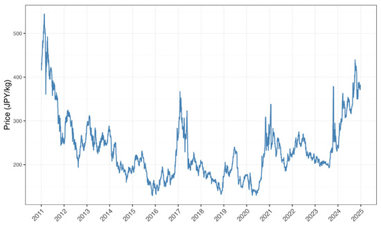
Figure 1.
Time series of TOCOM RSS3 front-month futures price.
The decomposition of daily returns into overnight and intraday components (Figure 2) provides the first visual evidence of their divergent nature. While both series exhibit volatility clustering, the overnight returns appear to contain more extreme, isolated jumps.
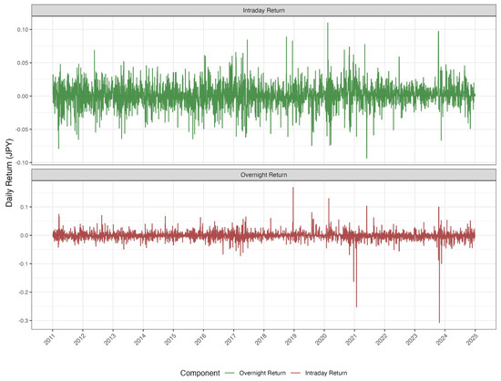
Figure 2.
Decomposition of daily return: overnight vs. intraday components.
Descriptive statistics for the return series (Table 3) confirm the preliminary visual analysis. All three series significantly deviate from normality, as evidenced by high kurtosis (>9) and Jarque–Bera test with p-values less than 0.0001. This justifies the use of a skewed Student-t distribution in subsequent volatility modeling. Crucially, the overnight return series exhibits the highest kurtosis (64.7901) and the most negative skewness (−2.0719), indicating a higher propensity for extreme negative jumps compared to the intraday component.
Table 3.
Descriptive statistics of return series.
4.1. The Inadequacy of the Monolithic Daily GARCH Model
A baseline GARCH(1,1) model with a skewed Student-t distribution was estimated on the aggregate daily return series. The model exhibited high volatility persistence . However, its out-of-sample performance, evaluated using a rolling-window value-at-risk (VaR) forecast at the 5% significance level, was deficient. The model recorded 142 VaR violations 6.7%, significantly exceeding the expected 105.7 breaches of 5%. Both the Kupiec unconditional coverage test likelihood ratio statistic LR.uc = 11.94, p-value = 0.001 and the Christoffersen conditional coverage test (LR.cc = 14.07, p-value = 0.001) decisively rejected the null hypothesis of correct model specification. This failure is not unique to the standard GARCH(1,1) specification; as demonstrated in Section 4.5, more complex models like EGARCH, IGARCH, and GJR-GARCH also fail when applied to the aggregated daily series. Furthermore, applying the regulatory Basel “Traffic Light” framework, these monolithic daily models fall squarely into the “red zone” due to the systematic and significant excess of VaR violations, which would trigger a punitive scaling factor for regulatory capital. This systematic underestimation of tail risk underscores the fundamental failure of a monolithic modeling approach and motivates the need for a disaggregated analysis.
4.2. Disentangling the Volatility Process: Intraday Reactivity vs. Overnight Jumps
To diagnose the source of the daily model’s failure, separate GARCH(1,1) models were estimated for the intraday and overnight return components. The results, presented in Table 4, reveal two starkly different volatility processes.
Table 4.
GARCH(1,1) Estimation Results for Return Components.
The intraday return series exhibits strong volatility responsiveness, as evidenced by a high ARCH coefficient (), indicating that current volatility reacts sharply to recent shocks. The GARCH term remains significant yet moderate (), demonstrating persistent but comparatively weaker volatility memory. The positive skewness parameter () suggests a proclivity for positive intraday price movements. Crucially, the Sign Bias Test results strongly confirm asymmetric volatility effects: with a joint statistic of (p-value ), there is highly significant negative sign bias, implying that negative shocks during trading hours amplify future volatility substantially more than positive shocks, consistent with a pronounced leverage effect. In contrast, overnight volatility is predominantly governed by the ARCH coefficient () with a near-zero and statistically insignificant GARCH term (). This pattern indicates a lack of traditional volatility persistence; instead, volatility arises from abrupt, large reactions to new information arriving during market closure—consistent with a jump-driven process. Furthermore, the Sign Bias Test (joint statistic , p-value ) does not detect significant leverage effects overnight, indicating that positive and negative overnight information shocks generate symmetric volatility responses.
The difference in the nature of their volatility is visually apparent in Figure 3, which plots the conditional volatilities for both components over time. The intraday volatility series shows smoother, more clustered evolution, while the overnight volatility is spikier, with sharp, isolated peaks corresponding to major informational events. This fundamental difference establishes the theoretical basis for the divergent Value-at-Risk performance.
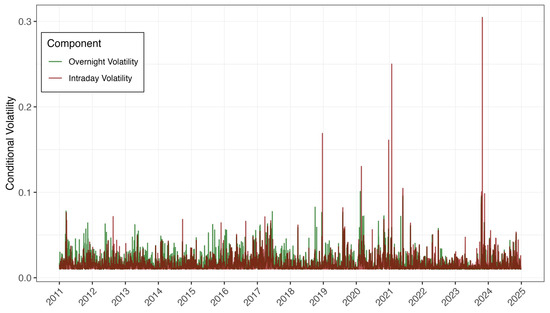
Figure 3.
Conditional volatility: overnight vs. intraday components.
4.3. Component-Specific Value-at-Risk (VaR) Performance
A critical test of our dichotomous volatility hypothesis examines whether separate modeling of intraday and overnight returns enhances risk assessment accuracy. The results of VaR backtesting at the 1% significance level are presented in Table 5.
Table 5.
VaR Backtest Results at 1% Significance Level.
The intraday GARCH model performs robustly. It yielded 15 VaR violations compared to an expected 21.1, with both the Kupiec unconditional coverage test (, ) and the Christoffersen conditional coverage test (, ) failing to reject the null hypothesis of correct conditional coverage. This performance would place the model in the “green zone” of the Basel regulatory framework, providing evidence that the standard GARCH framework adequately captures the risk dynamics of intraday price movements. Conversely, the overnight GARCH model exhibits poor performance. It incurred 37 violations against an expected 21.1, with the Kupiec test (, ) and Christoffersen test (, ) both decisively rejecting the null hypothesis.
Figure 4 provides a visual representation of these results, showing the VaR forecasts and exceedances for both components. The contrast is stark: the intraday VaR forecast envelope contains the returns smoothly, with exceedances (red points) scattered randomly. In contrast, the overnight VaR forecast is frequently breached, with exceedances often occurring in clusters during periods of market stress, visually confirming the model’s inability to predict the magnitude of overnight jumps.
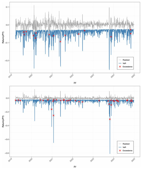
Figure 4.
(a) VaR forecast performance for intraday returns and (b) VaR forecast performance for overnight returns.
4.4. The Limited Role of Price Limits
An extended GARCH model incorporating a lagged price-limit dummy variable was estimated to assess its impact on daily volatility. The coefficient was positive but statistically insignificant (, ). This suggests that while price limits may contribute marginally to subsequent volatility, they are not the primary driver of the daily model’s failure. The results affirm that the core issue is the dichotomous nature of the volatility process itself, not the censoring mechanism.
4.5. Robustness Check with Alternative GARCH Specifications
To ensure the robustness of our core findings and address potential concerns about model specificity, we replicated the volatility and VaR analysis using a suite of alternative GARCH-family models. We employed the Exponential GARCH (EGARCH) model to capture asymmetric leverage effects, the GJR-GARCH model for an alternative parameterization of asymmetry, and the Integrated GARCH (IGARCH) to test a model with a fixed, high level of persistence. The results of the VaR backtests at the 1% significance level for both return components are consolidated in Table 6.
Table 6.
Robustness check: VaR backtest results for alternative GARCH models (1% significance level).
The backtesting results for the intraday return component, all model specifications— EGARCH, GJR-GARCH, and IGARCH—pass the VaR backtests, with Christoffersen p-values well above the 0.05 significance threshold (ranging from 0.1470 to 0.3300). This demonstrates that the reactive, persistent nature of intraday volatility is robustly captured by the standard GARCH toolkit. In stark contrast, for the overnight component, GJR-GARCH, and IGARCH models are decisively rejected (p-values < 0.05). The EGARCH model for overnight returns, while not statistically rejected (p-value = 0.3310), still produces a practically significant 28% more exceedances than expected (27 vs. 21.1). This pattern confirms that the failure of monolithic daily models and the inadequacy of modeling overnight returns with standard conditional variance equations are not artifacts of the baseline GARCH(1,1) model. Instead, they are a fundamental feature of the jump-driven overnight process, which is structurally different from the intraday process.
5. Discussion
5.1. Interpreting the Dichotomous Volatility Mechanism
Our results delineate a clear structural dichotomy in the TOCOM rubber futures market, resolving the puzzle of persistent VaR model failure. The intraday process exhibits the classic signatures of a liquid, sentiment-driven market: high ARCH () reactivity, significant volatility persistence, and a pronounced leverage effect where negative shocks disproportionately amplify future volatility (Bollerslev, 1987; Bollerslev & Zhou, 2006). This is consistent with the behavior of leveraged traders and loss aversion dynamics well-documented in equity markets. In stark contrast, the overnight process is a near-integrated, jump-driven phenomenon. The dominant ARCH term (), combined with a statistically insignificant GARCH term (), signifies a process with almost no memory of past volatility. Instead, it is defined by large, immediate reactions that reflect the discontinuous price discovery process as the market impounds information accumulated during the prolonged closure (Merton, 1976; Barndorff-Nielsen, 2004).
VaR backtesting reveals that the failure of overnight risk models is robust across most standard specifications. This is demonstrated by the decisive failure of multiple models (SGARCH, GJR-GARCH, IGARCH) at the 1% significance level, with all corresponding Kupiec p-values well below 0.005, registering at 0.0017, 0.0010, and 0.0020, respectively. However, the notable exception of the EGARCH model, which successfully passed the backtest (p-value = 0.2180), suggests that while the jump-like nature of overnight returns poses a challenge to symmetric GARCH models, specifications that can capture asymmetric news impacts may offer marginal improvements. Nonetheless, the catastrophic failure of the other models underscores the fundamental unreliability of the standard GARCH framework for this risk component. The market closure creates a discrete interval for global information—from Thai weather and Chinese industrial data to overnight moves in oil and equities—to accumulate. The subsequent opening auction impounds this information in a lumpy, discontinuous adjustment. The symmetry of this effect (no significant sign bias) suggests a relatively efficient, albeit abrupt, repricing to fundamental value, unmediated by the emotional and mechanistic trading of the continuous session.
This dichotomy is the root cause of the monolithic model’s failure. A standard daily GARCH model erroneously imposes a structure of smooth volatility clustering on a series that is, in fact, a mixture of a reactive, asymmetric intraday process and a jump-driven, symmetric overnight process. This conflation leads to a systematic underestimation of tail risk, which originates predominantly from the jump component.
5.2. Pragmatic and Regulatory Implications for Risk Management
Our findings carry immediate and consequential implications for practice, exposing a critical flaw in the prevailing reliance on a single daily VaR measure. The systematic underestimation of overnight jump risk provides a false sense of security. A trader hedging a long position may find their intraday VaR models are accurate, only to be consistently exposed to gap risk at the open that is not captured by their risk systems. This can lead to unexpected margin calls and liquidity shortfalls. Our analysis underscores a critical tension: price limit mechanisms, while designed to curb intraday panic, may inadvertently foster systemic undercapitalization against overnight gap risk. The robust failure of all monolithic daily GARCH models in Section 4.1, placing them in the Basel “red zone”, demonstrates that conventional internal models are blind to such discontinuities.
We therefore advocate a paradigm shift from a monolithic to a two-tiered risk management framework, whereby intraday risk continues to be modeled effectively using established techniques such as GARCH or historical simulation applied to intraday returns, which our robustness checks confirm are consistently adequate (Basel “green zone”). While overnight risk requires specialized treatment for jump dynamics through approaches such as Extreme Value Theory (EVT) for modeling the tail behavior of overnight returns (McNeil & Frey, 2000), stressed historical simulation based on worst-case empirical overnight jumps or the maintenance of a static capital buffer calibrated to conservative assumptions about maximum plausible overnight gaps (e.g., 5–8%). From a regulatory standpoint, this analysis underscores a critical tension: price limit mechanisms, while designed to curb intraday panic, may inadvertently foster systemic undercapitalization against overnight gap risk. Accordingly, regulators and standard-setting bodies such as the Basel Committee should recognize this issue. Oversight frameworks should encourage or mandate the adoption of component-specific modeling to ensure that capital adequacy genuinely reflects the true nature of risk exposure.
5.3. Theoretical Enrichment and Macroeconomic Signaling
Beyond its practical utility, this study enriches the theoretical literature. We provide a concrete empirical case where market microstructure—specifically, trading hours and exchange architecture—fundamentally determines the time-series properties of asset prices, a factor often abstracted away in theoretical models (Easley et al., 1997). Furthermore, the overnight return series can be interpreted as a high-frequency, market-based measure of “news impact” on a key industrial commodity. Analyzing the drivers of these jumps—by linking them to specific news events or moves in correlated asset classes—could unlock valuable insights into the global rubber market’s price formation process and its deeper integration into the world economy, offering a novel lens for macroeconomic analysis.
5.4. Limitations and Strategic Avenues for Future Research
Naturally, this work suggests several fruitful research pathways. While we characterize the jump process, explicitly modeling its fundamental drivers using news analytics or high-frequency data from correlated markets (e.g., Brent oil futures, equities) is a logical next step. The generalizability of this dichotomy to other commodities with similar trading structures (e.g., other TOCOM contracts, Chinese commodity futures) remains an essential empirical question. Furthermore, methodological advancements, such as applying formal Markov-switching GARCH models (Panagiotidis et al., 2022) to endogenously estimate regime transitions between “normal” and “jump” regimes directly from the daily series would represent a significant technical refinement of our proposed framework. Finally, the role of price limits under alternative market conditions warrants further investigation.
6. Conclusions
This study has diagnosed the persistent failure of standard Value-at-Risk (VaR) models in the Tokyo Commodity Exchange (TOCOM) rubber futures market by identifying its root cause not as a mere econometric shortcoming, but as a fundamental structural feature of the market’s microstructure. Through the decomposition of returns, we have demonstrated that the canonical daily return is a composite of two statistically distinct and economically meaningful components: a reactive intraday return governed by sentiment-driven trading with persistent volatility and leverage effects, and a discontinuous overnight return that behaves as a jump process, efficiently incorporating global fundamental news released during market closure.
The empirical evidence is robust and unequivocal. Our analysis, expanded to include a suite of GARCH-family models (EGARCH, GJR-GARCH, IGARCH), confirms that while these frameworks adequately capture intraday risk, they catastrophically fail to forecast overnight jump risk when applied to the aggregated daily series. This systematic failure, which places monolithic daily models in the Basel “red zone” invalidates the conventional approach to risk measurement in this market and highlights a critical vulnerability for financial institutions, hedgers, and clearinghouses.
Our principal contribution is to move the field from diagnosis to solution. We propose a paradigm shift towards a two-tiered risk management framework that aligns modeling techniques with the underlying volatility process. This entails employing standard GARCH models for intraday risk and adopting jump-aware methodologies, such as Extreme Value Theory (EVT) or stressed scenarios, for overnight risk. This tailored approach promises significantly enhanced capital adequacy, more accurate margin requirements, and greater financial resilience for all market participants.
The implications of this research extend beyond the TOCOM rubber market. It serves as a critical case study, demonstrating how institutional microstructures—such as split trading sessions—can fundamentally determine asset price dynamics to a degree that renders standard financial models ineffective. It underscores the imperative for both researchers and practitioners to integrate a deep understanding of market architecture into econometric analysis and regulatory practice. Future research should focus on the formal integration of these components within a unified regime-switching framework, explicitly model the drivers of overnight jumps, and test the generalizability of this volatility dichotomy across other commodity futures markets with similar trading calendars.
Author Contributions
Conceptualization, C.C., S.M. and R.S.; methodology, C.C., S.M. and R.S.; software, C.C.; validation, C.C., S.M. and R.S.; formal analysis, C.C. and S.M.; investigation, C.C.; resources, C.C. and S.M.; data curation, C.C.; writing—original draft preparation, C.C.; writing—review and editing, C.C., S.M. and R.S.; visualization, C.C. and R.S.; supervision, S.M. and R.S. All authors have read and agreed to the published version of the manuscript.
Funding
This research received no external fundings.
Institutional Review Board Statement
Not applicable.
Informed Consent Statement
Not applicable.
Data Availability Statement
The raw data supporting the conclusions of this article will be made available by the authors on request.
Acknowledgments
This study was funded by the PSU-Graduate Studies Scholarship in the year 2024 (contract No. PSU_GSS 2567-031). This study also partially funded by the Faculty of Science and Technology, Prince of Songkla University, Pattani campus, Thailand. The authors gratefully acknowledge the helpful comments and suggestions provided by the reviewers, which have significantly improved the quality and clarity of this manuscript.
Conflicts of Interest
The authors declare no conflicts of interest.
Abbreviations
The following abbreviations are used in this manuscript:
| TOCOM | Tokyo Commodity Exchange |
| VaR | Value-at-Risk |
| EVT | Extreme Value Theory |
References
- Alim, W., Khan, N. U., Zhang, V. W., Cai, H. H., Mikhaylov, A., & Yuan, Q. (2024). Influence of political stability on the stock market returns and volatility: GARCH and EGARCH approach. Financial Innovation, 10(1), 139. [Google Scholar] [CrossRef]
- Andersen, T. G., & Bollerslev, T. (1997). Intraday periodicity and volatility persistence in financial markets. Journal of Empirical Finance, 4(2–3), 115–158. [Google Scholar] [CrossRef]
- Andersen, T. G., Bollerslev, T., Diebold, F. X., & Labys, P. (2003). Modeling and forecasting realized volatility. Econometrica, 71(2), 579–625. [Google Scholar] [CrossRef]
- Badescu, A., Cui, Z., & Ortega, J.-P. (2017). Non-affine GARCH option pricing models, variance-dependent kernels, and diffusion limits. Journal of Financial Econometrics, 15(4), 602–648. [Google Scholar] [CrossRef]
- Barndorff-Nielsen, O. E. (2004). Power and bipower variation with stochastic volatility and jumps. Journal of Financial Econometrics, 2(1), 1–37. [Google Scholar] [CrossRef]
- Basle Committee on Banking Supervision. (1996). Supervisory framework for the use of back-testing in conjunction with the internal models approach to market risk capital requirements. Available online: https://www.bis.org/publ/bcbs22.htm (accessed on 28 October 2025).
- Bollerslev, T. (1987). A conditionally heteroskedastic time series model for speculative prices and rates of return. The Review of Economics and Statistics, 69(3), 542–457. [Google Scholar] [CrossRef]
- Bollerslev, T., & Wooldridge, J. M. (1992). Quasi-maximum likelihood estimation and inference in dynamic models with time-varying covariances. Econometric Reviews, 11(2), 143–172. [Google Scholar] [CrossRef]
- Bollerslev, T., & Zhou, H. (2006). Volatility puzzles: A simple framework for gauging return-volatility regressions. Journal of Econometrics, 131(1–2), 123–150. [Google Scholar] [CrossRef]
- Chang, C. L., Khamkaew, T., McAleer, M., & Tansuchat, R. (2011). Modelling conditional correlations in the volatility of asian rubber spot and futures returns. Mathematics and Computers in Simulation, 81(7), 1482-–1490. [Google Scholar] [CrossRef]
- Cheema, M. A., Chiah, M., & Man, Y. (2022). Overnight returns, daytime reversals, and future stock returns: Is China different? Pacific-Basin Finance Journal, 74, 101809. [Google Scholar] [CrossRef]
- Chen, X., & Ghysels, E. (2010). News—Good or bad—And its impact on volatility predictions over multiple horizons. Review of Financial Studies, 24(1), 46–81. [Google Scholar] [CrossRef]
- Christoffersen, P. F. (1998). Evaluating interval forecasts. International Economic Review, 39(4), 841. [Google Scholar] [CrossRef]
- Ciner, C. (2002). Information content of volume: An investigation of Tokyo commodity futures markets. Pacific-Basin Finance Journal, 10(2), 201–215. [Google Scholar] [CrossRef]
- Easley, D., Kiefer, N. M., & O’Hara, M. (1997). One day in the life of a very common stock. Review of Financial Studies, 10(3), 805–835. [Google Scholar] [CrossRef]
- Engle, R. (2001). GARCH 101: The use of ARCH/GARCH models in applied econometrics. Journal of Economic Perspectives, 15(4), 157–168. [Google Scholar] [CrossRef]
- Engle, R. F. (1982). Autoregressive conditional heteroscedasticity with estimates of the variance of United Kingdom inflation. Econometrica, 50(4), 987–1007. [Google Scholar] [CrossRef]
- Engle, R. F., & Ng, V. K. (1993). Measuring and testing the impact of news on volatility. The Journal of Finance, 48(5), 1749–1778. [Google Scholar] [CrossRef]
- Engle, R. F., & Siriwardane, E. N. (2017). Structural GARCH: The volatility-leverage connection. The Review of Financial Studies, 31(2), 449–492. [Google Scholar] [CrossRef]
- Fama, E. F., & French, K. R. (1988). Dividend yields and expected stock returns. Journal of Financial Economics, 22(1), 3–25. [Google Scholar] [CrossRef]
- Galanos, A. (2025). rugarch: Univariate GARCH models [Computer software manual]. (R package version 1.5-4). Available online: http://cran.r-project.org/web/packages/rugarch (accessed on 15 July 2025).
- Glosten, L. R., Jagannathan, R., & Runkle, D. E. (1993). On the relation between the expected value and the volatility of the nominal excess return on stocks. The Journal of Finance, 48(5), 1779–1801. [Google Scholar] [CrossRef]
- Gorton, G., & Rouwenhorst, K. G. (2006). Facts and fantasies about commodity futures. Financial Analysts Journal, 62(2), 47–68. [Google Scholar] [CrossRef]
- Guermat, C., & Harris, R. D. (2002). Forecasting value at risk allowing for time variation in the variance and kurtosis of portfolio returns. International Journal of Forecasting, 18(3), 409–419. [Google Scholar] [CrossRef]
- Hansen, P. R., & Lunde, A. (2005). A forecast comparison of volatility models: Does anything beat a GARCH(1,1)? Journal of Applied Econometrics, 20(7), 873–889. [Google Scholar] [CrossRef]
- Hansen, P. R., & Lunde, A. (2006). Realized variance and market microstructure noise. Journal of Business & Economic Statistics, 24(2), 127–161. [Google Scholar] [CrossRef]
- Huang, X., & Tauchen, G. (2005). The relative contribution of jumps to total price variance. Journal of Financial Econometrics, 3(4), 456–499. [Google Scholar] [CrossRef]
- Jiang, Y., Jiang, C., Nie, H., & Mo, B. (2019). The time-varying linkages between global oil market and China’s commodity sectors: Evidence from DCC-GJR-GARCH analyses. Energy, 166, 577–586. [Google Scholar] [CrossRef]
- Jondeau, E., & Rockinger, M. (2003). Testing for differences in the tails of stock-market returns. Journal of Empirical Finance, 10(5), 559–581. [Google Scholar] [CrossRef]
- Kang, S. H., Tiwari, A. K., Albulescu, C. T., & Yoon, S.-M. (2019). Exploring the time-frequency connectedness and network among crude oil and agriculture commodities V1. Energy Economics, 84, 104543. [Google Scholar] [CrossRef]
- Kilian, L., & Murphy, D. P. (2014). The role of inventories and speculative trading in the global market for crude oil. Journal of Applied Econometrics, 29(3), 454–478. [Google Scholar] [CrossRef]
- Kupiec, P. H. (1995). Techniques for verifying the accuracy of risk measurement models. The Journal of Derivatives, 3(2), 73–84. [Google Scholar] [CrossRef]
- Li, M., & Yang, L. (2013). Modeling the volatility of futures return in rubber and oil—A copula-based GARCH model approach. Economic Modelling, 35, 576–581. [Google Scholar] [CrossRef]
- Ljung, G. M., & Box, G. E. (1980). Analysis of variance with autocorrelated observations. Scandinavian Journal of Statistics, 7(4), 172–180. [Google Scholar]
- McNeil, A. J., & Frey, R. (2000). Estimation of tail-related risk measures for heteroscedastic financial time series: An extreme value approach. Journal of Empirical Finance, 7(3–4), 271–300. [Google Scholar] [CrossRef]
- Merton, R. C. (1976). Option pricing when underlying stock returns are discontinuous. Journal of Financial Economics, 3(1–2), 125–144. [Google Scholar] [CrossRef]
- Nelson, D. B. (1991). Conditional heteroskedasticity in asset returns: A new approach. Econometrica, 59(2), 347–370. [Google Scholar] [CrossRef]
- Panagiotidis, T., Papapanagiotou, G., & Stengos, T. (2022). On the volatility of cryptocurrencies. Research in International Business and Finance, 62, 101724. [Google Scholar] [CrossRef]
- Srisuksai, P. (2020). The rubber pricing model: Theory and evidence. The Journal of Asian Finance, Economics and Business, 7(11), 13–22. [Google Scholar] [CrossRef]
- Tripathi, J. S., & Rengifo, E. W. (2025). The impact of earnings announcements before and after regular market hours on asset price dynamics in the fintech era. Journal of Risk and Financial Management, 18(2), 75. [Google Scholar] [CrossRef]
- Yeap, X. W., & Lean, H. H. (2022). Trading activities and the volatility of return on Malaysian crude palm oil futures. Journal of Risk and Financial Management, 15(1), 34. [Google Scholar] [CrossRef]
Disclaimer/Publisher’s Note: The statements, opinions and data contained in all publications are solely those of the individual author(s) and contributor(s) and not of MDPI and/or the editor(s). MDPI and/or the editor(s) disclaim responsibility for any injury to people or property resulting from any ideas, methods, instructions or products referred to in the content. |
© 2025 by the authors. Licensee MDPI, Basel, Switzerland. This article is an open access article distributed under the terms and conditions of the Creative Commons Attribution (CC BY) license (https://creativecommons.org/licenses/by/4.0/).