
Artificial Intelligence for Cluster Analysis: Case Study of Transport Companies in Czech Republic

Abstract
:1. Introduction
2. Literature Research
3. Materials and Methods
3.1. Dataset
- Specification of the company: company registration number (IČO), name of the company;
- Information on the company: date of resources, beginning and end of the period, number of months of the financial statement;
- Financial statements: balance sheet, profit and loss list (PLL).
- The value “0” was added in empty cells: the table containing the generated data was selected, and “Replace” was used to replace fill in all empty cells in the table with the value 0.
- It is necessary to add another column “EBIT” by adding the column “EBT” and “Interest payable”.
- The beginning and end of the period outside the period of 2015–2018 were removed.
- The columns and rows containing zero entries, the columns with zero variance, and duplicate rows were removed (“Data”—“Remove duplicates”—“by company registration number”). Subsequently, the entities (in rows) for which the data for the period other than 12 months (different accounting periods) needed to be removed, as well as the non-numeric entries.
- ROA and ROE were calculated, where ROA is expressed as a ratio of EBIT and assets and ROE is the ratio of EAT and equity.
- All necessary components for calculating EVA Equity (from the point of view of shareholders) wsas calculated: risk-free return—rf; indicators characterizing the company size—rLA; indicators characterizing the production power—rentrepreneurship; XP; indicators characterizing the relationship between assets and liabilities—rfinstab; and weighted average costs of capital—WACC (risk-free return + indicators characterizing the company size + indicators characterizing the production power + indicators characterizing the relationship between assets and liabilities) according to (Vochozka 2020):Alternative costs of equity— according to (MPO 2016):where
- UZ—financial resources (equity and interest-bearing debt capital);
- A—assets;
- VK—equity;
- BU—bank loans;
- O—bonds;
- —interest rate, can be marked i (interest);
- d—income tax rate (can be marked t—tax).
Financial resources—UZ (equity + issued long-term bonds + issued short-term bonds + bank loans and financial assistance), rate of corporate tax—d (according to a relevant year—since 2010, the rate has been 19%). - After calculating all necessary components, EVA Equity was calculated as follows:
- It was necessary to carry out the so-called data cleansing by removing nonsensical and extreme values; subsequently, non-numerical entries of EVA Equity needed to be removed, e.g., those with the error message claiming that it is not possible to divide by zero.
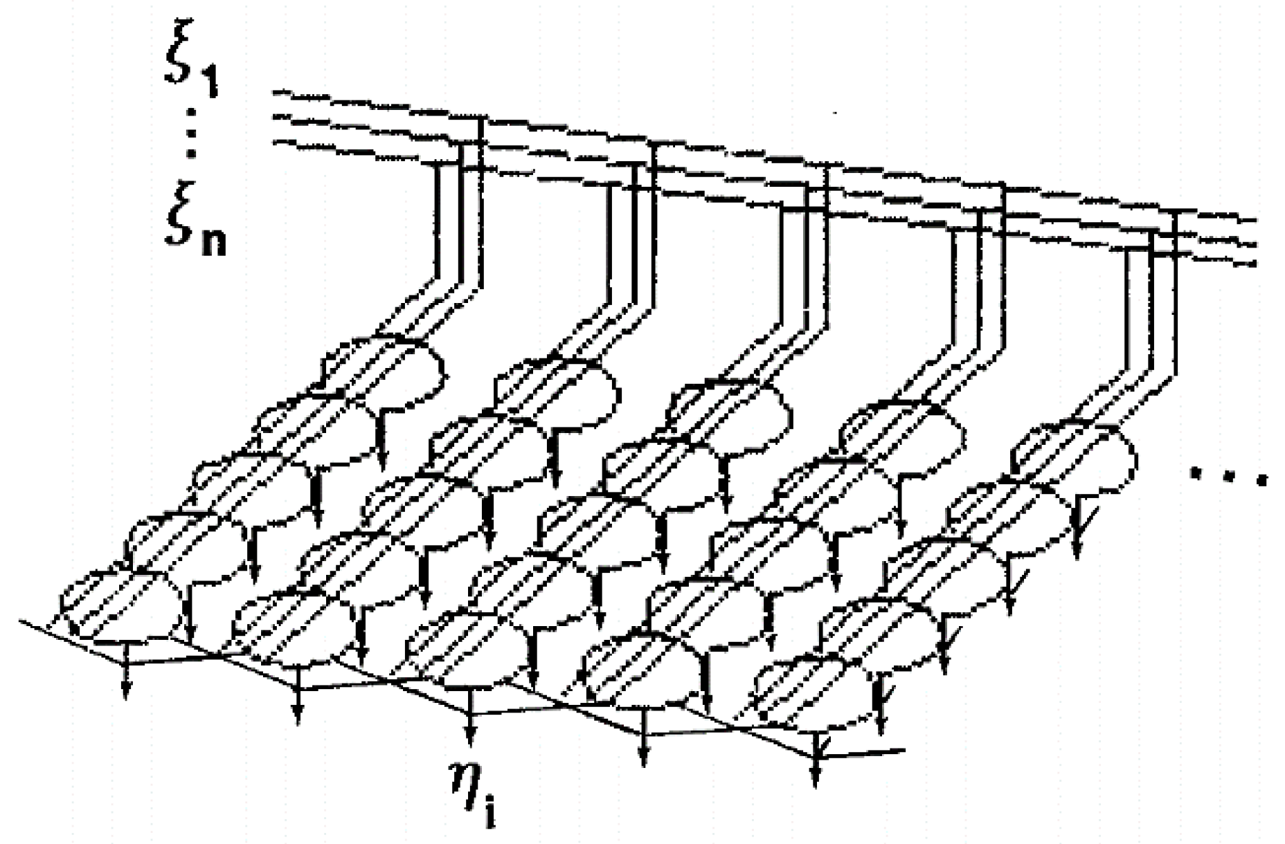
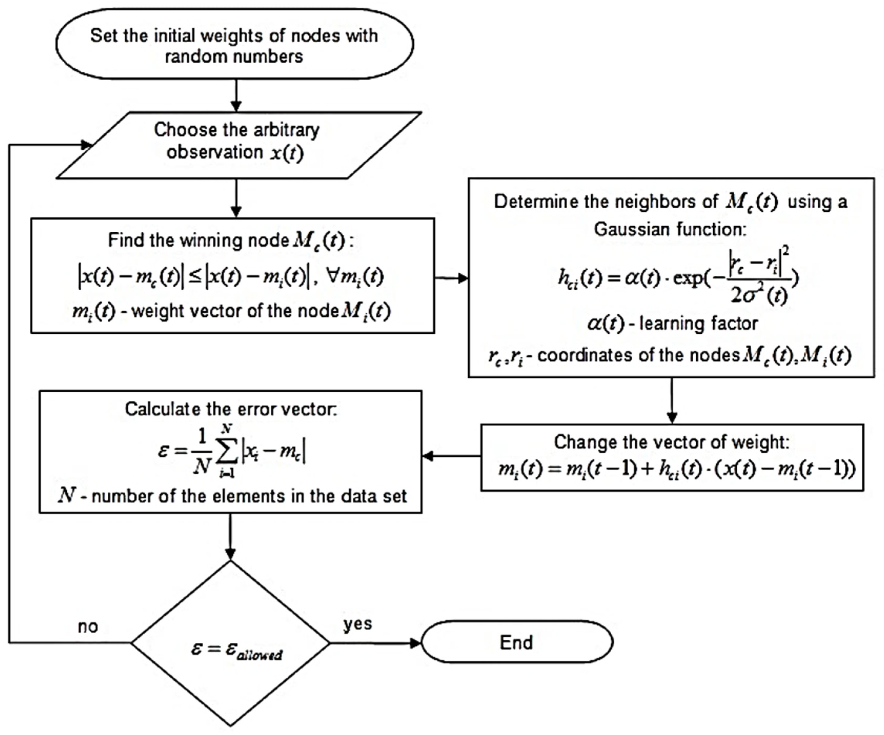
3.2. Methods
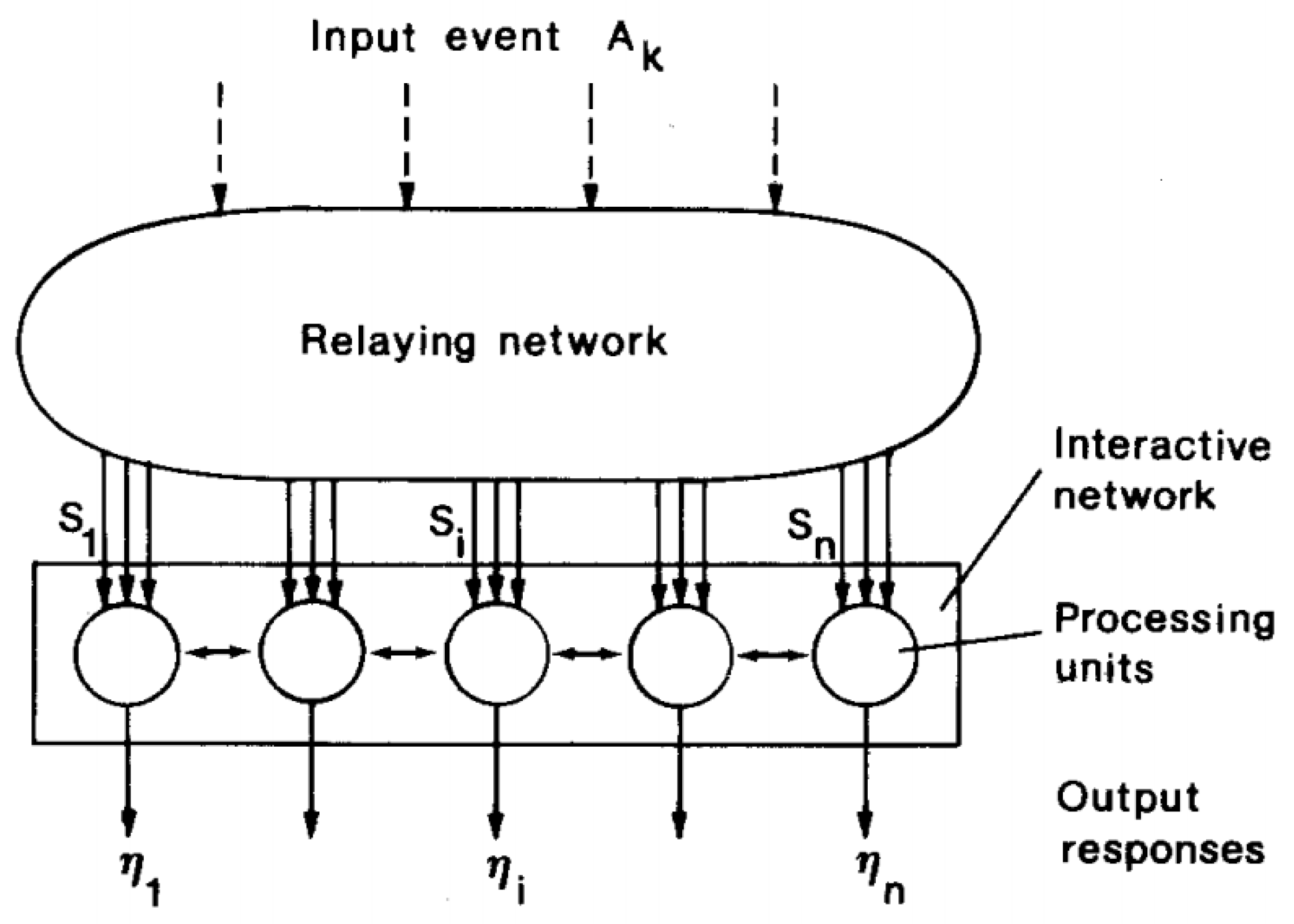
- A set of processor units that receive coherent inputs from the event space and create simple distinguishing functions of their input signals;
- A mechanism that compares distinguishing functions and selects the unit with the highest functional value;
- A kind of local interaction that simultaneously activates the selected drive and its closest neighbors;
- An adaptive process that causes the parameters of activated units to increase their distinguishing functional values related to simultaneous input.
- -
- total assets;
- -
- fixed assets;
- -
- sales;
- -
- operating profit or loss.
4. Results
4.1. Dataset
- Specification of the company: company registration number (IČO), name of the company;
- Information on the company: date of resources, beginning and end of the period, and number of months of the financial statement;
- Financial statements: balance sheet, profit, and loss account (PLL).
4.2. Training of Neural Networks and Its Results
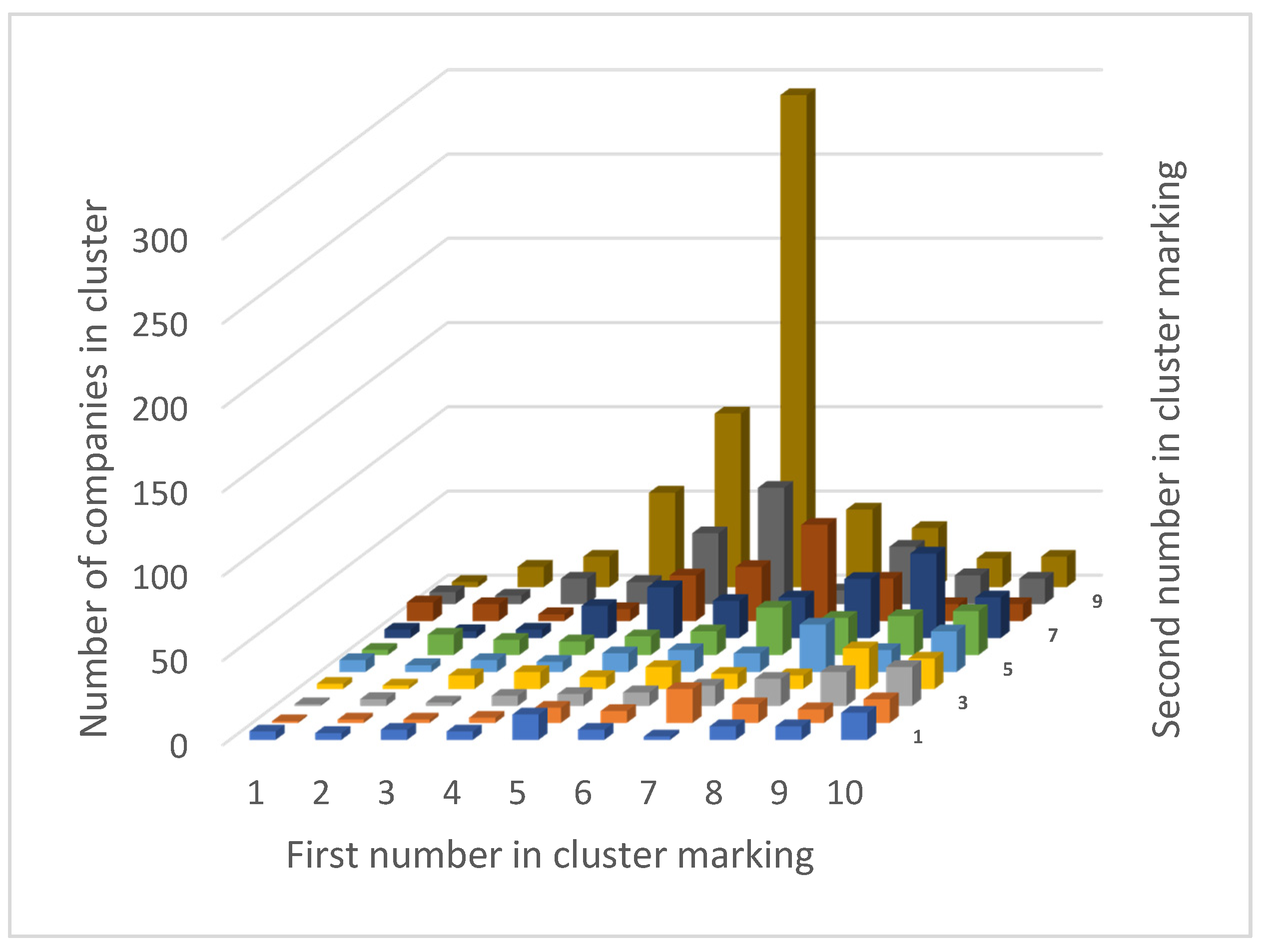
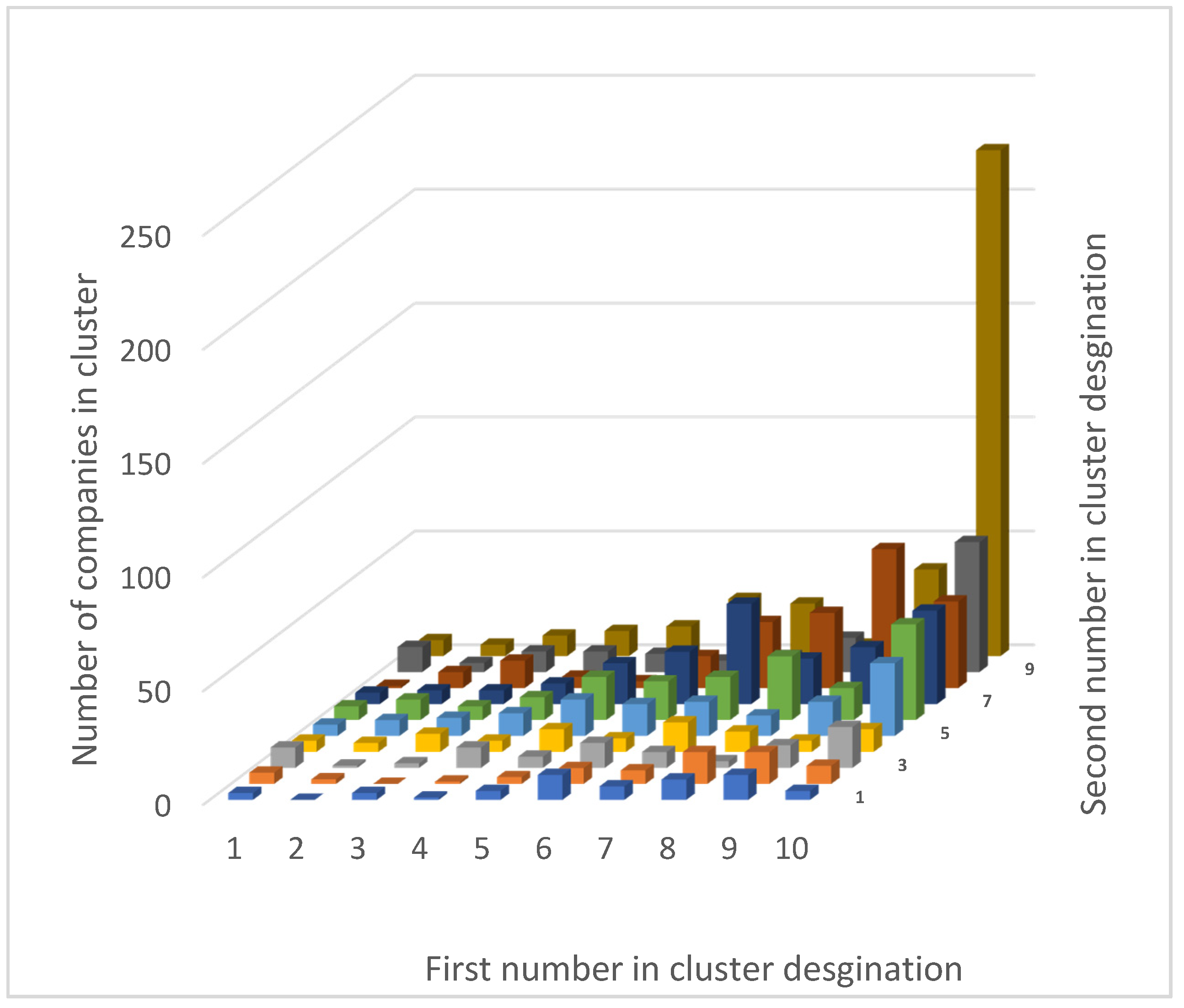
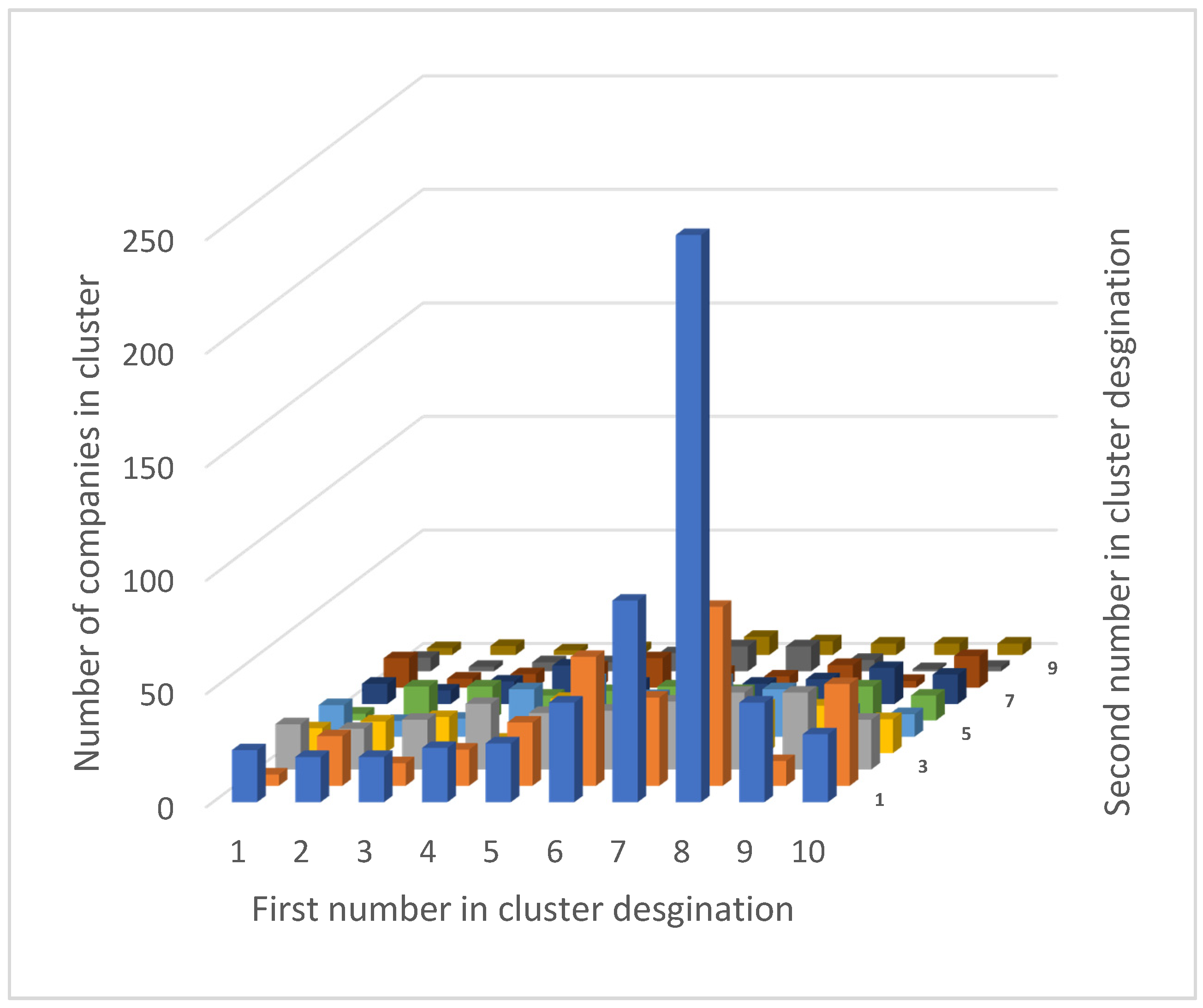
4.3. Analysis of Strongest Cluster
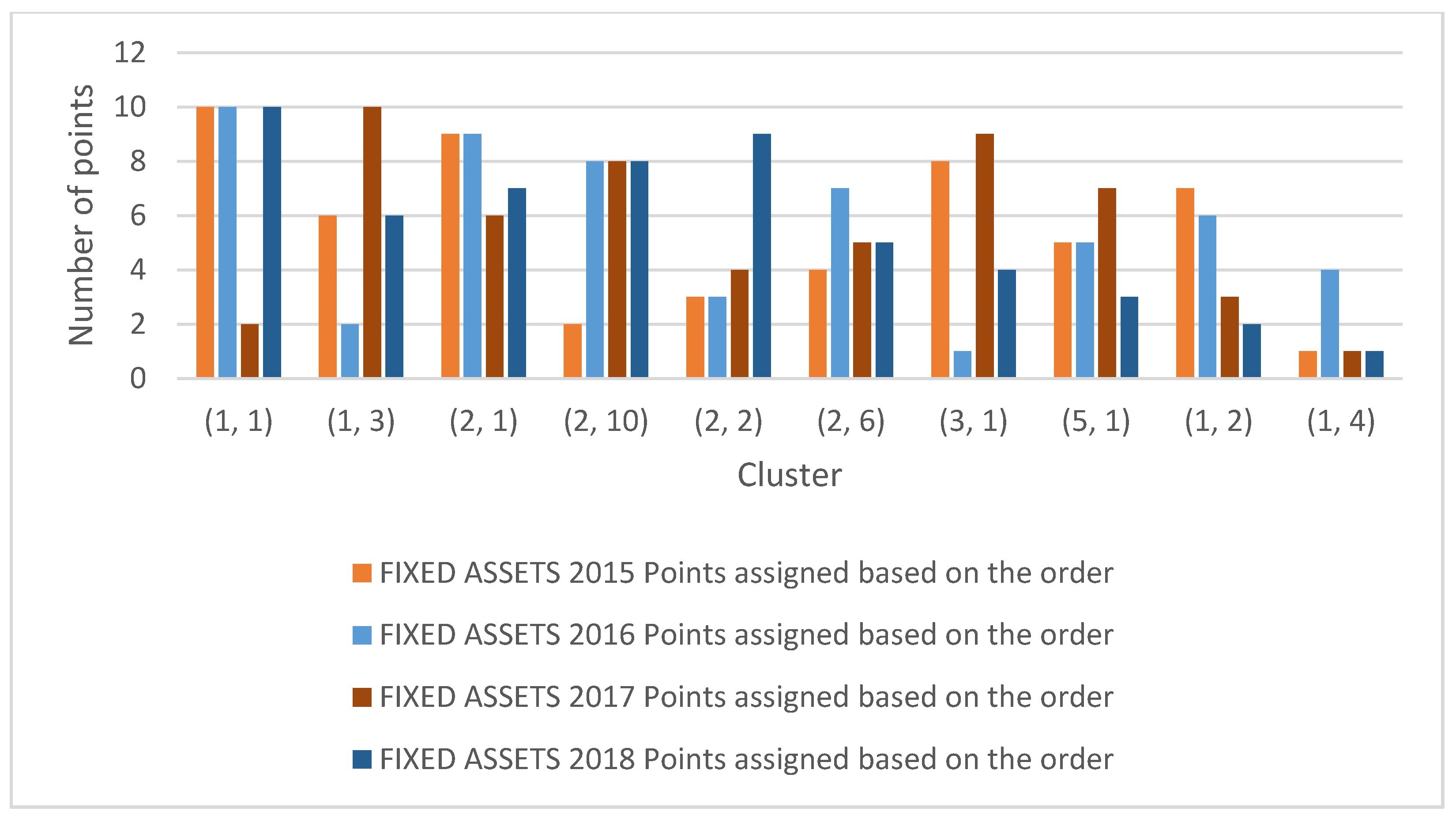
4.4. Order of Clusters and Their Scoring
4.5. The Strongest Cluster of the Overall Ranking
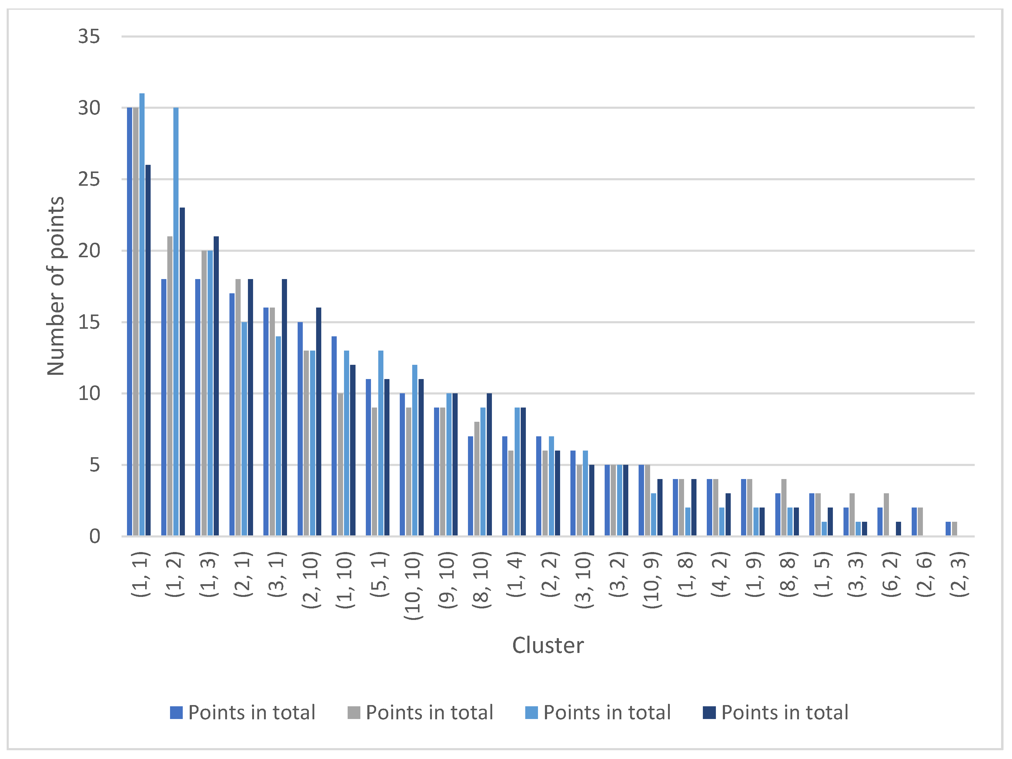
4.6. Ranking of Strongest Clusters
4.6.1. Analysis of Companies in Cluster (1, 1)
4.6.2. Analysis of Selected Companies from Cluster (1, 1) and Their Participation in the Creation of the Selected Components
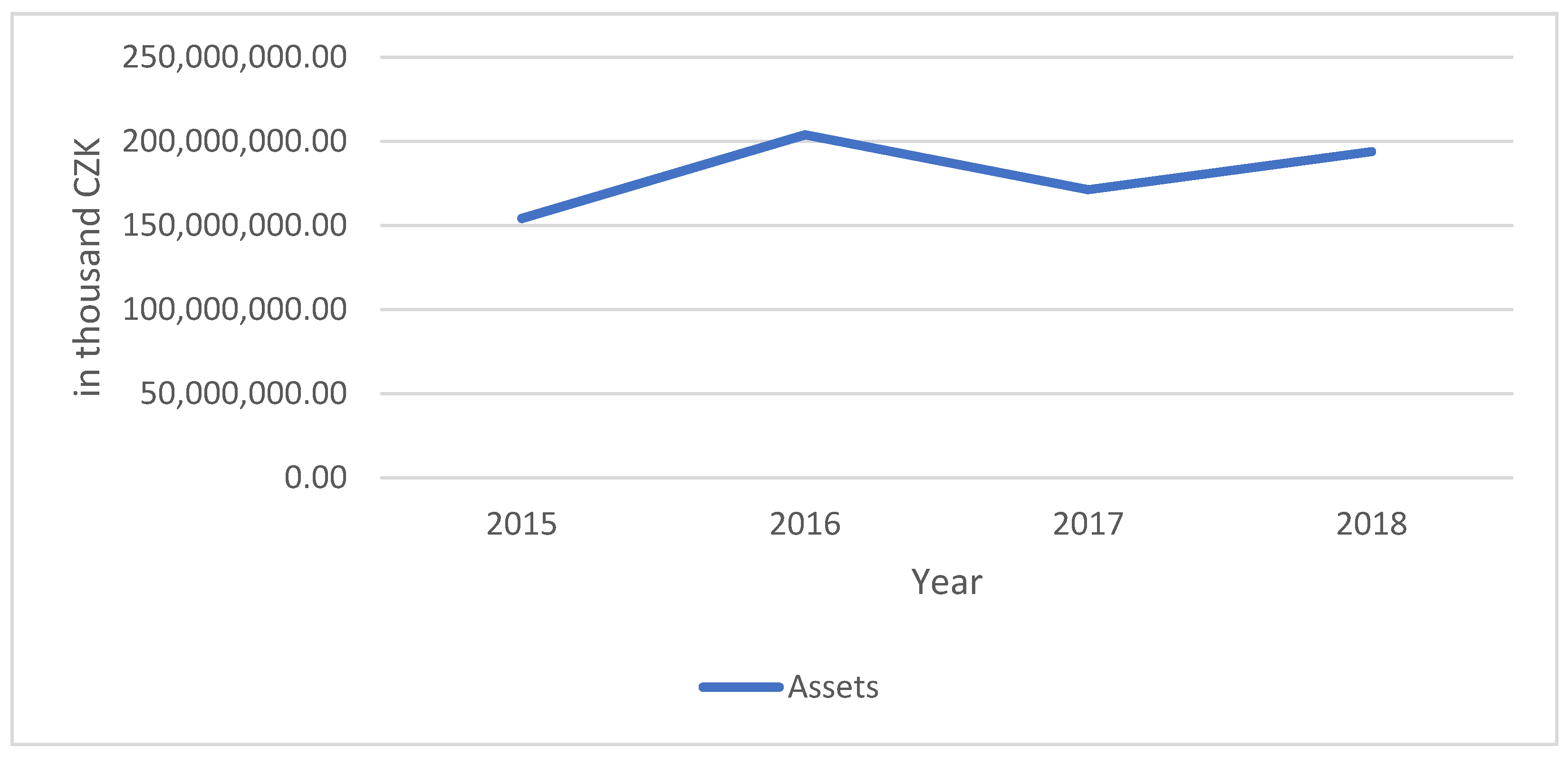
4.7. Financial Analysis of Selected Companies
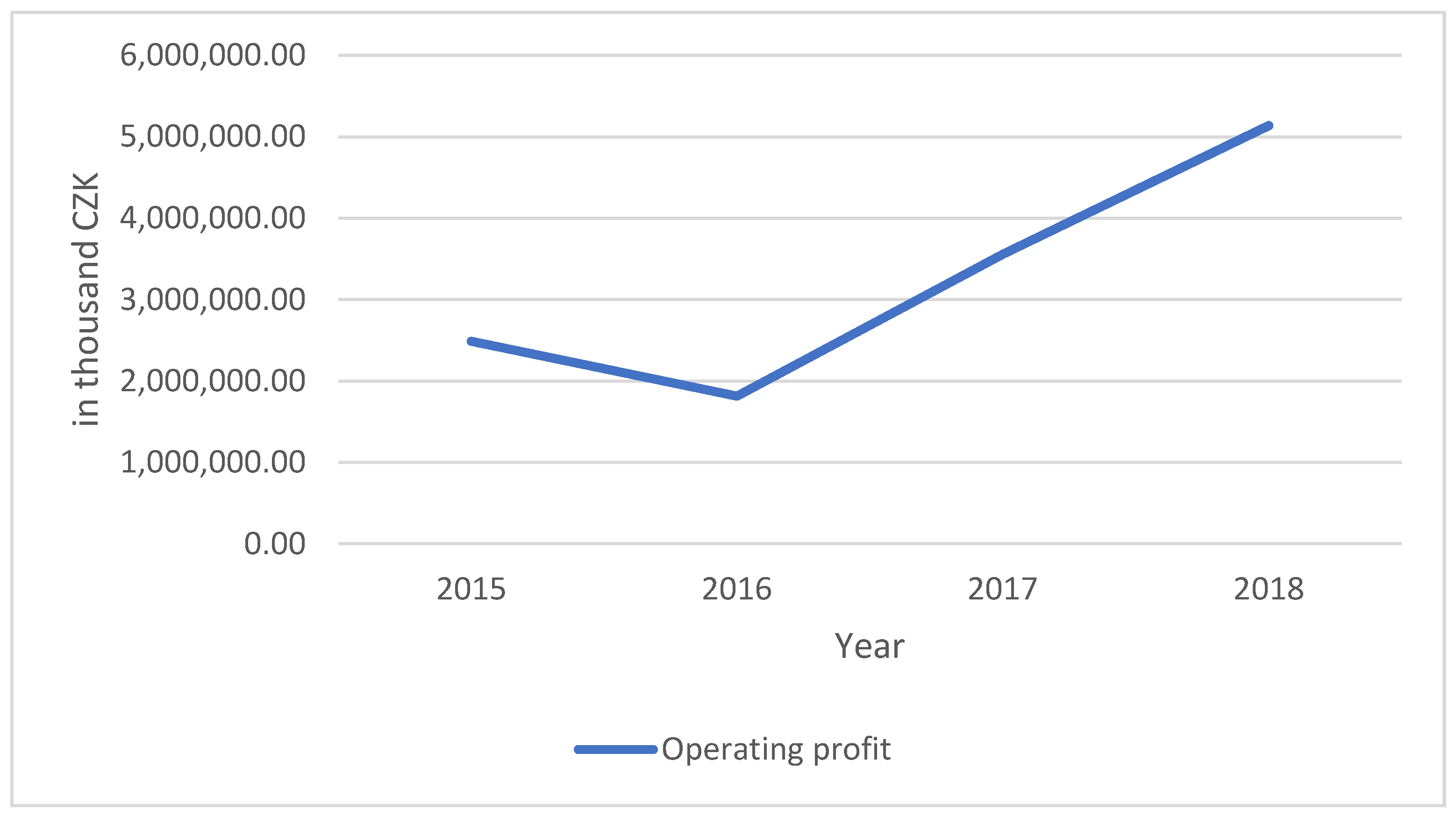
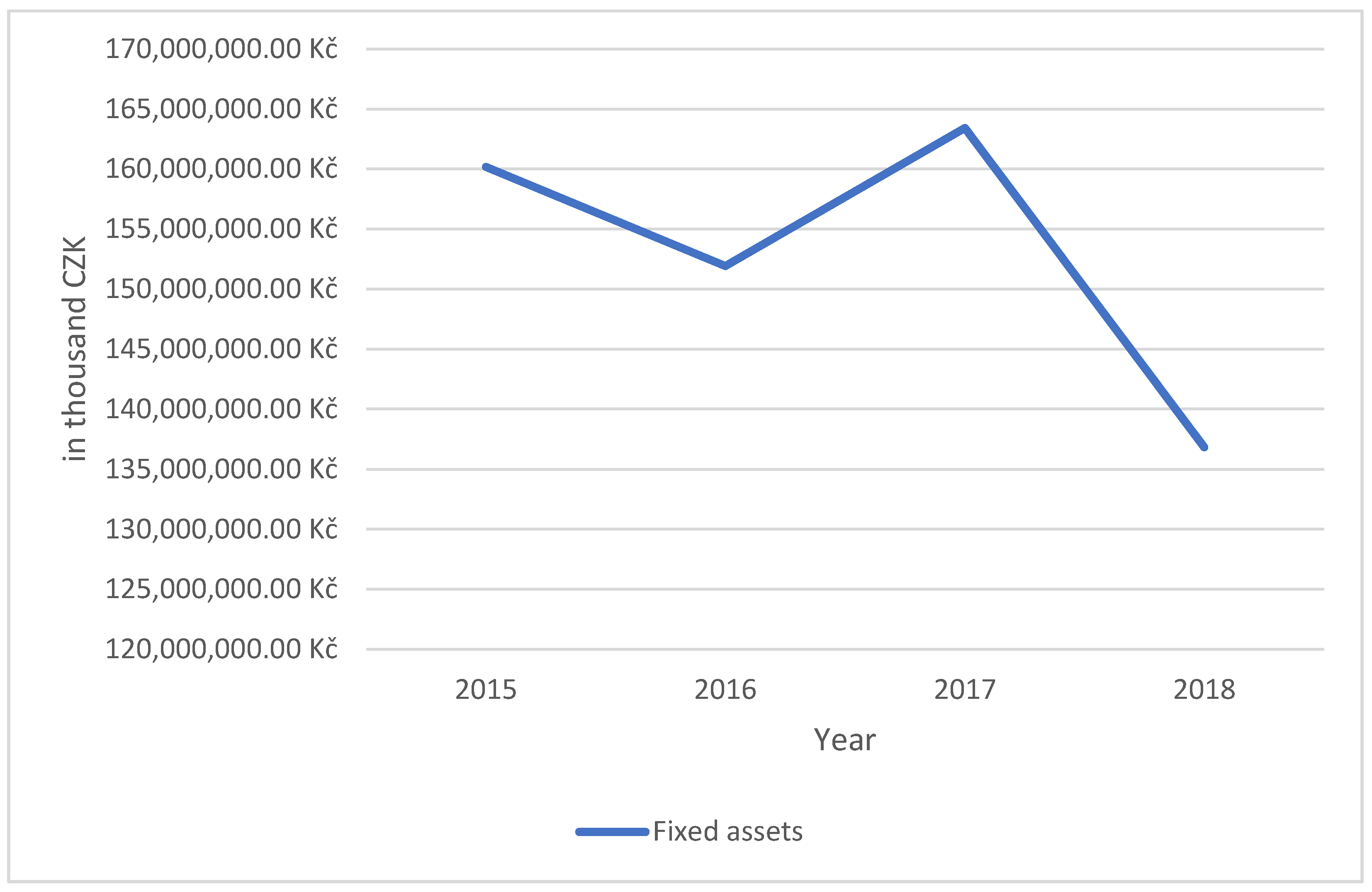
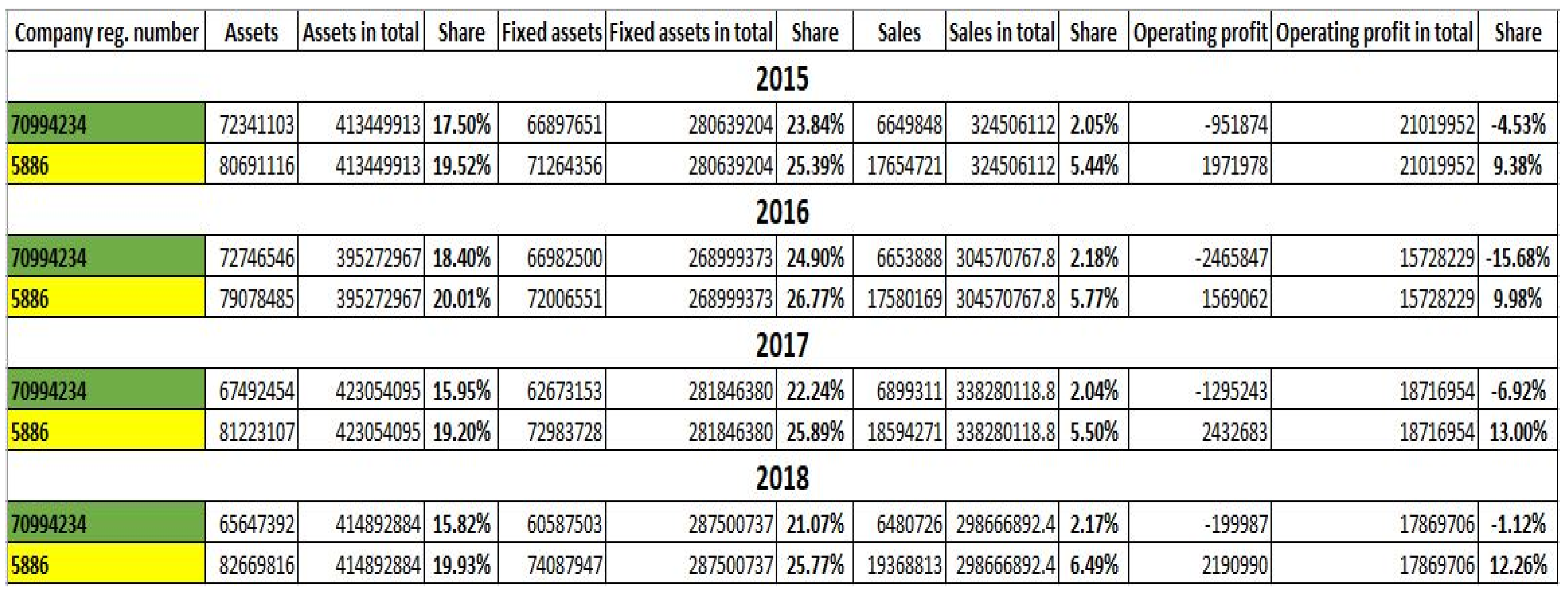
4.7.1. Company with the Registration Number 70994234—Správa Železnic, Státní Podnik
4.7.2. Company with the Registration Number 5886—Dopravní Podnik hl. Města Prahy
5. Discussion
6. Conclusions
Funding
Institutional Review Board Statement
Informed Consent Statement
Data Availability Statement
Acknowledgments
Conflicts of Interest
Appendix A

| Ratio | Unit of Measurement | Year | |||||||||||
|---|---|---|---|---|---|---|---|---|---|---|---|---|---|
| 2008 | 2009 | 2010 | 2011 | 2012 | 2013 | 2014 | 2015 | 2016 | 2017 | ||||
| Number of active companies | 41,785 | 42,094 | 41,873 | 41,232 | 40,064 | 38,944 | 38,610 | 38,159 | 39,016 | 39,791 | |||
| Number of employed persons in total—in natural persons | persons | 305,801 | 292,676 | 284,021 | 279,027 | 267,444 | 262,886 | 264,532 | 271,389 | 281,680 | 287,996 | ||
| From the above: | Average registered number of employees—in natural persons | persons | 261,887 | 248,932 | 240,301 | 234,335 | 225,906 | 220,100 | 221,430 | 227,885 | 236,524 | 242,654 | |
| Average registered number of employees —equivalent | persons | 256,886 | 245,192 | 236,696 | 231,002 | 222,648 | 217,010 | 218,578 | 225,023 | 233,348 | 239,954 | ||
| Average gross monthly wage per natural person | CZK | 22,233 | 22,332 | 22,351 | 22,480 | 22,686 | 22,657 | 23,172 | 23,871 | 24,963 | 26,656 | ||
| Average gross monthly wage per 1 equivalent person | CZK | 22,666 | 22,672 | 22,692 | 22,804 | 23,018 | 22,980 | 23,475 | 24,175 | 25,302 | 26,956 | ||
| Net turnover (Total revenues) | million CZK | 631,182 | 539,302 | 580,318 | 591,781 | 608,224 | 619,828 | 649,497 | 634,861 | 647,091 | 679,345 | ||
| including | Sales of products and services and sales of goods | million CZK | 541,165 | 470,076 | 512,957 | 528,654 | 543,574 | 547,580 | 575,238 | 572,396 | 584,773 | 615,837 | |
| including | Sales of products and services, | million CZK | 455,460 | 399,637 | 438,805 | 449,196 | 449,240 | 447,626 | 476,725 | 499,679 | 516 451 | 547,284 | |
| Sales of goods | million CZK | 85,705 | 70,440 | 74,152 | 79,459 | 94,334 | 99,954 | 98,513 | 72,717 | 68 322 | 68,553 | ||
| Other operating income | million CZK | 73,739 | 57,600 | 52,002 | 54,057 | 56,341 | 61,924 | 67,724 | 56,389 | 52,768 | 53,165 | ||
| Income including trade margin | million CZK | 461,202 | 404,484 | 443,254 | 454,118 | 454,000 | 452,271 | 481,334 | 504,236 | 521,183 | 552,565 | ||
| Costs in total | million CZK | 606,610 | 525,103 | 551,443 | 567,717 | 586,484 | 600,027 | 624,401 | 604,586 | 617,987 | 648,669 | ||
| including | Consumption of material and energy, costs of services | million CZK | 332,138 | 284,139 | 308,370 | 321,987 | 324,396 | 323,289 | 342,302 | 350,662 | 362,646 | 385,880 | |
| Cost of goods sold | million CZK | 81,813 | 66,878 | 70,798 | 75,670 | 91,027 | 96,658 | 95,262 | 69,485 | 65,025 | 64,899 | ||
| Other operational costs | million CZK | 45,756 | 34,619 | 38,149 | 37,427 | 44,507 | 46,209 | 56,728 | 42,652 | 36,932 | 34,525 | ||
| Personnel costs | million CZK | 98,286 | 93,806 | 91,816 | 89,730 | 86,727 | 85,400 | 87,520 | 92,766 | 100,849 | 110,595 | ||
| including | Wages without UN | million CZK | 69,870 | 66,709 | 64,452 | 63,213 | 61,499 | 59,842 | 61,572 | 65,279 | 70,851 | 77,618 | |
| Trade margin | million CZK | 3892 | 3561 | 3354 | 3788 | 3308 | 3295 | 3251 | 3232 | 3297 | 3653 | ||
| Share of trade margin on sales of goods | % | 4.5 | 5.1 | 4.5 | 4.8 | 3.5 | 3.3 | 3.3 | 4.4 | 4.8 | 5.3 | ||
| Added value | million CZK | 129,064 | 120,346 | 134,884 | 132,130 | 129,605 | 128,981 | 139,032 | 153,574 | 158,537 | 166,685 | ||
| Earnings for current accounting year | million CZK | 24,572 | 14,199 | 28,875 | 24,064 | 21,740 | 19,801 | 25,096 | 30,274 | 29,104 | 30,677 | ||
| Net assets | million CZK | 554,067 | 551,091 | 559,267 | 540,713 | 537,802 | 548,815 | 559,505 | 572,898 | 592,724 | 605,721 | ||
| including | Fixed intangible assets (net) | million CZK | 3478 | 3685 | 3576 | 5911 | 5927 | 5716 | 5477 | 5296 | 5714 | 5631 | |
| Fixed tangible assets (net) | million CZK | 344,678 | 348,973 | 346,560 | 328,366 | 334,975 | 326,886 | 331,924 | 335,636 | 338,762 | 340,331 | ||
| Fixed financial assets (net) | million CZK | 29,079 | 28,499 | 29,195 | 27,802 | 22,559 | 28,845 | 31,274 | 33,026 | 33,118 | 34,488 | ||
| Inventories without advances provided (net) | million CZK | 12,140 | 11,005 | 9893 | 10,398 | 10,369 | 9896 | 9971 | 9581 | 10,723 | 10,544 | ||
| receivables (net) | million CZK | 108,115 | 104,888 | 114,827 | 115,860 | 107,675 | 115,193 | 109,395 | 113,498 | 127,337 | 134,200 | ||
| Liabilities | million CZK | 554,067 | 551,091 | 559,267 | 540,713 | 537,802 | 548,815 | 559,505 | 572,898 | 592,724 | 605,721 | ||
| including | equity | million CZK | 342,575 | 343,616 | 352,957 | 317,118 | 308,863 | 310,668 | 284,611 | 293,220 | 312,711 | 323,313 | |
| liabilities | million CZK | 195,036 | 192,106 | 191,197 | 209,726 | 216,818 | 226,346 | 262,906 | 266,519 | 266,689 | 268,377 | ||
| Acquisition of fixed tangible and intangible assets | million CZK | 59,782 | 42,473 | 45,149 | 56,050 | 47,716 | 50,857 | 46,651 | 51,919 | 49,219 | 42,720 | ||
Appendix B
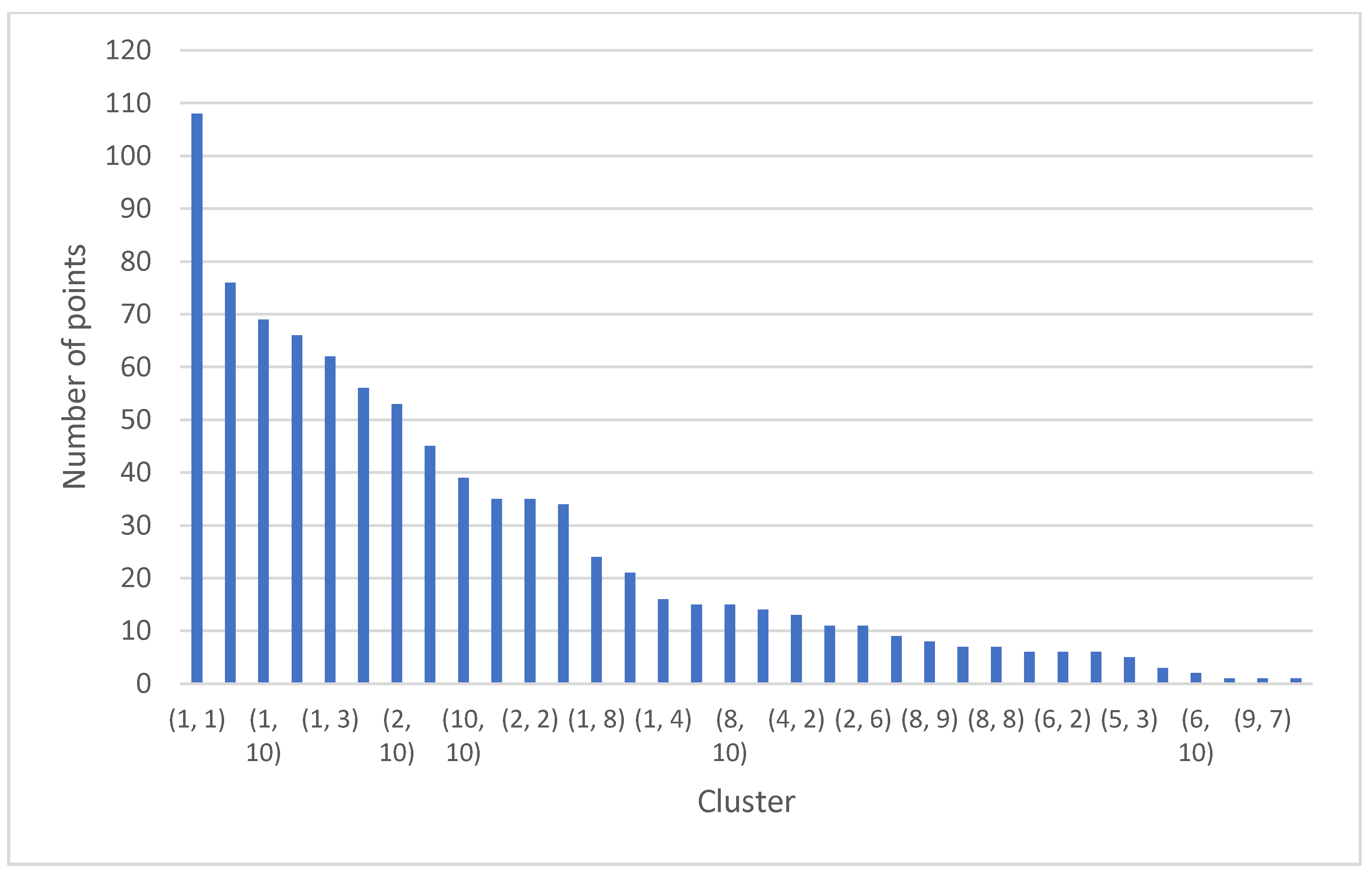
| Clusters | Number of Points in Total |
|---|---|
| (1, 1) | 108 |
| (1, 2) | 76 |
| (1, 10) | 69 |
| (2, 1) | 66 |
| (1, 3) | 62 |
| (3, 1) | 56 |
| (2, 10) | 53 |
| (1, 9) | 45 |
| (10, 10) | 39 |
| (9, 10) | 35 |
| (2, 2) | 35 |
| (5, 1) | 34 |
| (1, 8) | 24 |
| (10, 9) | 21 |
| (1, 4) | 16 |
| (3, 10) | 15 |
| (8, 10) | 15 |
| (1, 5) | 14 |
| (4, 2) | 13 |
| (3, 2) | 11 |
| (2, 6) | 11 |
| (2, 3) | 9 |
| (8, 9) | 8 |
| (2, 9) | 7 |
| (8, 8) | 7 |
| (3, 4) | 6 |
| (6, 2) | 6 |
| (3, 3) | 6 |
| (5, 3) | 5 |
| (2, 4) | 3 |
| (6, 10) | 2 |
| (6, 1) | 1 |
| (9, 7) | 1 |
| (1, 7) | 1 |
References
- Abdelkafi, Inès, Manel Zribi, and Rochdi Feki. 2018. New Classification of Developed and Emerging Countries Based on the Effects of Subprime Crises: Kohonen Map Method. Journal of the Knowledge Economy 9: 908–27. [Google Scholar] [CrossRef]
- Awrejcewicz, Jan, Yu B. Lind, Aigul R. Kabirova, Liana F. Nurislamova, Irek M. Gabaidullin, and Rinat A. Mulyukov. 2011. Prediction of drilling fluids loss during oil and gas wells construction. Paper presented at the 11th Conference on Dynamical Systems—Theory and Applications, Lódz, Poland, December 5–8; pp. 163–70. [Google Scholar]
- Bakoben, Maha, Tony Bellotti, and Niall Adams. 2017. Identification of credit risk based on cluster analysis of account behaviours. Journal of the Operational Research Society 71: 775–83. [Google Scholar] [CrossRef]
- Cahyana, Bambang Eka, Umar Nimran, Hamidah Nayati Utami, and Mohammad Iqbal. 2020. Hybrid cluster analysis of customer segmentation of sea transportation users. Journal of Economics, Finance and Administrative Science 25: 321–37. [Google Scholar] [CrossRef]
- Cho, Sungbin, Jinhwa Kim, and Jae Kwon Bae. 2009. An integrative model with subject weight based on neural network learning for bankruptcy prediction. Expert Systems with Applications 36: 403–10. [Google Scholar] [CrossRef]
- Du Jardin, Philippe, and Eric Séverin. 2012. Forecasting financial failure using a kohonen map: A comparative study to improve model stability over time. European Journal of Operational Research 221: 378–96. [Google Scholar] [CrossRef] [Green Version]
- Feranecova, Adela, Martina Sabolova, and Peter Remias. 2016. Cluster analysis of automotive industry companies. Actual Problems of Economics 182: 95–102. [Google Scholar]
- Harchli, Fidae, ES-Safi Abdelatif, and Ettaouil Mohamed. 2014. Novel method to optimize the architecture of kohonen’s topological maps and clustering. Paper presented at the 2nd IEEE International Conference on Logistics Operations Management, GOL 2014, Rabat, Morocco, June 5–7; pp. 8–14. [Google Scholar] [CrossRef]
- Kohonen, Teuvo. 1982. Self-organized formation of topologically correct feature maps. Biological Cybernetics 43: 59–69. [Google Scholar] [CrossRef]
- Kohonen, Teuvo. 1986. Self-organization, memorization, and associative recall of sensory information by brain-like adaptive networks. International Journal of Quantum Chemistry 30: 209–21. [Google Scholar] [CrossRef]
- Lakhawat, Piyush, and Arun K. Somani. 2017. Big Data Cluster Analysis: A Study of Existing Techniques and Future Directions. In Big Data Analytics: Tools and Technology for Effective Planning, 1st ed. Edited by Arun K. Somani and Ganesh Chandra Deka. New York: Chapman and Hall/CRC, p. 413. [Google Scholar]
- Liashenko, Olena, Tetyana Kravets, and Tetiana Verhai. 2018. Estimation of the Production Potential of Ukraine’s Regions Using Kohonen Neural Network. Paper presented at the CEUR Workshop Proceedings, 2105, ICTERI 2018, Kyiv, Ukraine, May 14–17; pp. 19–34. [Google Scholar]
- Li, Hui, Hong Lu-Yao, Zhou Qing, and Yu Hai-Jie. 2015. The assisted prediction modelling frame with hybridisation and ensemble for business risk forecasting and an implementation. International Journal of Systems Science 46: 2072–86. [Google Scholar] [CrossRef]
- MPO. 2016. Metodika Výpočtu—Analytické Materiály a Statistiky [Online]. Available online: https://www.mpo.cz/assets/cz/rozcestnik/analyticke-materialy-a-statistiky/2016/11/metodika-vypoctu.pdf (accessed on 21 June 2021).
- Rayala, Venkat, and Satyanarayan Reddy Kalli. 2021. Big data clustering using improvised fuzzy C-means clustering. Revue d’Intelligence Artificielle 34: 701–8. [Google Scholar] [CrossRef]
- Rodrigue, Jean-Paul, Claude Comtois, and Brian Slack. 2013. The Geography of Transport Systems, 3rd ed. New York: Routledge, p. 432. [Google Scholar]
- Rowland, Zuzana, and Jaromír Vrbka. 2016. Using artificial neural networks for prediction of key indicators of a company in global world. In Globalization and Its Socio-Economic Consequences, 16th International Scientific Conference Proceedings. Žilina: EDP Sciences, pp. 1896–903. [Google Scholar]
- Stehel, Vojtěch, Jakub Horák, and Marek Vochozka. 2019. Prediction of institutional sector development and analysis of enterprises active in agriculture. E a M: Ekonomie a Management 22: 103–18. [Google Scholar] [CrossRef]
- Svobodová, Hana, Antonín Věžník, and Eduard Hofmann. 2013. Vybrané kapitoly ze socioekonomické geographie České republiky, 1st ed. Brno: Masarykova Univerzita, p. 163. [Google Scholar]
- Tyukhova, Elena, and Dmitry Sizykh. 2019. The cluster analysis method as an instrument for selection of securities in the construction of an investment portfolio. Paper presented at the 2019 12th International Conference “Management of Large-Scale System Development”, MLSD 2019, Moscow, Russia, October 1–3; p. 621. [Google Scholar]
- Vahalík, Bohdan, and Michaela Staníčková. 2016. Key factors of foreign trade competitiveness: Comparison of the EU and BRICS by factor and cluster analysis. Society and Economy 38: 295–317. [Google Scholar] [CrossRef]
- Vochozka Marek. 2020. Metody Komplexního Hodnocení Podniku, 2nd ed. Prague: Grada Publishing. [Google Scholar]
- Vochozka, Marek, and Veronika Machová. 2017. Enterprise value generators in the building industry. SHS Web of Conferences 39: 01029. [Google Scholar] [CrossRef] [Green Version]


| Company ID | Source Date | Beginning of Period | End of Period | Number of Months | Position 2015 |
|---|---|---|---|---|---|
| 5885 | 20160725 | 20150901 | 20151231 | 12 | (1, 1) |
| 28244532 | 20160725 | 20130901 | 20151231 | 12 | (2, 2) |
| 50993531 | 20160725 | 20130001 | 20151231 | 12 | (2, 1) |
| 80753811 | 20150725 | 20150101 | 20151231 | 12 | (1, 2) |
| 24622191 | 20170724 | 20150901 | 20151231 | 12 | (1, 3) |
| 25663135 | 20170115 | 20150901 | 20951231 | 12 | (1, 1) |
| 27092077 | 20150620 | 20130901 | 20151231 | 12 | (2, 1) |
| 25438307 | 20160704 | 20150001 | 20151231 | 12 | (5, 1) |
| 49710571 | 20150815 | 20130001 | 20151231 | 12 | (2, 1) |
| 28396678 | 20150604 | 20150901 | 20951231 | 12 | (1, 1) |
| 25506881 | 20190704 | 20130901 | 20151231 | 12 | (2, 1) |
| 25317075 | 20150101 | 20150901 | 20951231 | 12 | (2, 10) |
| 47134983 | 20150505 | 20150901 | 20151231 | 12 | (1, 1) |
| 28202375 | 20170227 | 20130901 | 20151231 | 12 | (2, 9) |
| 2015 | 2016 | 2017 | 2018 | ||||||||||||
|---|---|---|---|---|---|---|---|---|---|---|---|---|---|---|---|
| Cluster | Company ID | Assets (in Thousand CZK) | Rank | Cluster | Company ID | Assets (in Thousand CZK) | Rank | Cluster | Company ID | Assets (in Thousand CZK) | Rank | Cluster | Company ID | Assets (in Thousand CZK) | Rank |
| (1, 1) | 5 | 193,983,526 | 1 | (1, 1) | 4 | 171,374,111 | 1 | (10, 10) | 5 | 204,003,403 | 1 | (1, 1) | 3 | 154,281,306 | 1 |
| (2, 1) | 4 | 49,520,740 | 2 | (1, 3) | 4 | 34,370,036 | 2 | (9, 10) | 5 | 41,379,275 | 2 | (1, 2) | 5 | 56,310,851 | 2 |
| (3, 1) | 6 | 13,980,772 | 3 | (2, 1) | 2 | 23,429,904 | 3 | (2, 10) | 4 | 13,061,112 | 3 | (3, 1) | 3 | 43,923,622 | 3 |
| (2, 10) | 12 | 10,575,537 | 4 | (1, 10) | 13 | 17,644,871 | 4 | (8, 10) | 5 | 13,044,534 | 4 | (5, 1) | 4 | 32,299,614 | 4 |
| (2, 2) | 2 | 8,418,137 | 5 | (1, 4) | 5 | 10,231,255 | 5 | (3, 10) | 2 | 9,053,831 | 5 | (1, 3) | 9 | 12,570,680 | 5 |
| (1, 2) | 1 | 8,083,333 | 6 | (3, 2) | 6 | 8,736,490 | 6 | (10, 9) | 2 | 8,510,567 | 6 | (1, 10) | 7 | 9,475,552 | 6 |
| (5, 1) | 15 | 7,906,670 | 7 | (1, 2) | 2 | 8,415,907 | 7 | (1, 8) | 13 | 8,065,330 | 7 | (4, 2) | 1 | 6,992,077 | 7 |
| (1, 3) | 1 | 6,402,191 | 8 | (1, 5) | 11 | 7,725,963 | 8 | (8, 8) | 10 | 6,946,246 | 8 | (1, 9) | 11 | 5,517,543 | 8 |
| (2, 6) | 12 | 5,468,181 | 9 | (3, 3) | 14 | 7,274,867 | 9 | (1, 10) | 3 | 6,841,701 | 9 | (6, 2) | 7 | 4,918,045 | 9 |
| (1, 4) | 3 | 5,308,183 | 10 | (2, 3) | 11 | 6,764,269 | 10 | (1, 9) | 6 | 6,641,100 | 10 | (2, 2) | 2 | 4,274,520 | 10 |
| Assets 2015 | ||
|---|---|---|
| Row Labels | Sum of Order | Number of Ranking Points |
| (1, 1) | 1 | 10 |
| (1, 3) | 8 | 3 |
| (1, 4) | 10 | 1 |
| (2, 1) | 2 | 9 |
| (2, 10) | 4 | 7 |
| (2, 2) | 5 | 6 |
| (3, 1) | 3 | 8 |
| (5, 1) | 7 | 4 |
| (1, 2) | 6 | 5 |
| (2, 6) | 9 | 2 |
| 1 | 2 | 3 | 4 | 5 | 6 | 7 | 8 | 9 | 10 | |
|---|---|---|---|---|---|---|---|---|---|---|
| 1 | 5 | 4 | 6 | 5 | 15 | 6 | 2 | 8 | 8 | 16 |
| 2 | 1 | 2 | 2 | 3 | 9 | 7 | 20 | 11 | 8 | 14 |
| 3 | 1 | 4 | 2 | 6 | 7 | 8 | 12 | 16 | 20 | 23 |
| 4 | 3 | 2 | 8 | 10 | 7 | 13 | 9 | 8 | 24 | 18 |
| 5 | 7 | 4 | 7 | 6 | 11 | 13 | 11 | 28 | 13 | 24 |
| 6 | 3 | 12 | 9 | 8 | 11 | 14 | 28 | 22 | 23 | 26 |
| 7 | 5 | 4 | 5 | 19 | 30 | 22 | 24 | 35 | 50 | 24 |
| 8 | 11 | 10 | 4 | 7 | 27 | 32 | 57 | 25 | 10 | 10 |
| 9 | 7 | 5 | 15 | 13 | 42 | 69 | 8 | 34 | 17 | 15 |
| 10 | 3 | 12 | 18 | 56 | 103 | 292 | 46 | 35 | 17 | 18 |
| 1 | 2 | 3 | 4 | 5 | 6 | 7 | 8 | 9 | 10 | |
|---|---|---|---|---|---|---|---|---|---|---|
| 1 | 4 | 2 | 1 | 7 | 4 | 7 | 6 | 10 | 1 | 13 |
| 2 | 2 | 4 | 6 | 4 | 10 | 4 | 3 | 10 | 5 | 7 |
| 3 | 4 | 11 | 14 | 14 | 15 | 11 | 12 | 17 | 4 | 8 |
| 4 | 5 | 18 | 13 | 19 | 25 | 16 | 6 | 22 | 16 | 13 |
| 5 | 11 | 16 | 12 | 26 | 16 | 19 | 11 | 18 | 35 | 7 |
| 6 | 8 | 10 | 18 | 13 | 37 | 32 | 20 | 22 | 23 | 29 |
| 7 | 12 | 22 | 16 | 11 | 10 | 32 | 36 | 47 | 24 | 33 |
| 8 | 12 | 6 | 17 | 10 | 12 | 13 | 16 | 54 | 38 | 38 |
| 9 | 7 | 4 | 15 | 22 | 23 | 31 | 7 | 79 | 31 | 5 |
| 10 | 13 | 8 | 13 | 13 | 26 | 34 | 32 | 220 | 12 | 10 |
| 1 | 2 | 3 | 4 | 5 | 6 | 7 | 8 | 9 | 10 | |
|---|---|---|---|---|---|---|---|---|---|---|
| 1 | 23 | 20 | 20 | 24 | 26 | 44 | 89 | 289 | 44 | 30 |
| 2 | 5 | 22 | 10 | 16 | 28 | 57 | 39 | 79 | 11 | 45 |
| 3 | 20 | 18 | 22 | 29 | 25 | 26 | 30 | 34 | 34 | 22 |
| 4 | 11 | 14 | 16 | 6 | 24 | 12 | 24 | 21 | 21 | 15 |
| 5 | 14 | 7 | 8 | 21 | 25 | 18 | 25 | 21 | 12 | 10 |
| 6 | 3 | 15 | 15 | 11 | 13 | 15 | 13 | 12 | 15 | 11 |
| 7 | 9 | 6 | 10 | 17 | 9 | 17 | 9 | 11 | 16 | 13 |
| 8 | 13 | 4 | 6 | 9 | 13 | 7 | 5 | 10 | 3 | 14 |
| 9 | 6 | 2 | 4 | 4 | 8 | 11 | 11 | 5 | 1 | 2 |
| 10 | 3 | 4 | 2 | 3 | 6 | 8 | 6 | 5 | 5 | 5 |
| 1 | 2 | 3 | 4 | 5 | 6 | 7 | 8 | 9 | 10 | |
|---|---|---|---|---|---|---|---|---|---|---|
| 1 | 3 | 0 | 3 | 1 | 4 | 11 | 6 | 9 | 11 | 4 |
| 2 | 5 | 2 | 0 | 1 | 3 | 7 | 6 | 14 | 14 | 8 |
| 3 | 9 | 1 | 2 | 9 | 5 | 11 | 7 | 3 | 10 | 18 |
| 4 | 5 | 4 | 8 | 5 | 10 | 6 | 13 | 9 | 5 | 10 |
| 5 | 5 | 7 | 8 | 10 | 16 | 14 | 15 | 9 | 15 | 32 |
| 6 | 6 | 9 | 6 | 10 | 19 | 17 | 19 | 28 | 14 | 42 |
| 7 | 5 | 6 | 6 | 9 | 18 | 23 | 44 | 20 | 25 | 41 |
| 8 | 1 | 7 | 12 | 5 | 3 | 14 | 29 | 33 | 61 | 38 |
| 9 | 11 | 4 | 9 | 9 | 8 | 5 | 7 | 15 | 14 | 57 |
| 10 | 7 | 5 | 9 | 11 | 13 | 25 | 23 | 5 | 38 | 222 |
| Clusters | Number of Companies | Sum of Total Assets—Thousand CZK |
|---|---|---|
| (1, 1) | 5 | 193,983,526 |
| (2, 1) | 4 | 49,520,740 |
| (3, 1) | 6 | 13,980,772 |
| (2, 10) | 12 | 10,575,537 |
| (2, 2) | 2 | 8,418,137 |
| (1, 2) | 1 | 8,083,333 |
| (5, 1) | 15 | 7,906,670 |
| (1, 3) | 1 | 6,402,191 |
| (2, 6) | 12 | 5,468,181 |
| Clusters | Number of Companies | Sum of Total Assets—In Thousand CZK |
|---|---|---|
| (1, 1) | 4 | 171,374,111 |
| (1, 3) | 4 | 34,370,036 |
| (2, 1) | 2 | 23,429,904 |
| (1, 10) | 13 | 17,644,871 |
| (1, 4) | 5 | 10,231,255 |
| (3, 2) | 6 | 8,736,490 |
| (1, 2) | 2 | 8,415,907 |
| (1, 5) | 11 | 7,725,963 |
| (3, 3) | 14 | 7,274,867 |
| (2, 3) | 11 | 6,764,269 |
| Clusters | Number of Companies | Sum of Total Assets—Thousand CZK |
|---|---|---|
| (10, 10) | 5 | 204,003,403 |
| (9, 10) | 5 | 41,379,275 |
| (2, 10) | 4 | 13,061,112 |
| (8, 10) | 5 | 13,044,534 |
| (3, 10) | 2 | 9,053,821 |
| (10, 9) | 2 | 8,510,567 |
| (1, 8) | 13 | 8,065,330 |
| (8, 8) | 10 | 6,946,246 |
| (1, 10) | 3 | 6,841,701 |
| (1, 9) | 6 | 6,641,100 |
| Company ID | Name of the Company | Source Date | Beginning of the Period | End of the Period | Number of Months of Financial Statemens | Position 2015 | Position 2016 | Position 2017 | Position 2018 |
|---|---|---|---|---|---|---|---|---|---|
| 70994234 | SŽDC | 20170502 | 20150101 | 20151231 | 12 | (1, 1) | (1, 1) | (10, 10) | (1, 1) |
| 5886 | Dopavní podnik hl. m. Prahy | 20160725 | 20150101 | 20151231 | 12 | (1, 1) | (1, 1) | (10, 10) | (1, 1) |
| Clusters | Number of Companies | Sum of Total Assets—Thousand CZK |
|---|---|---|
| (1, 1) | 3 | 154,281,306 |
| (1, 2) | 5 | 56,310,851 |
| (3, 1) | 3 | 43,923,622 |
| (5, 1) | 4 | 32,299,614 |
| (1, 3) | 9 | 12,570,680 |
| (1, 10) | 7 | 9,475,552 |
| (4, 2) | 1 | 6,992,077 |
| (1, 9) | 11 | 5,517,543 |
| (6, 2) | 7 | 4,918,045 |
| (2, 2) | 2 | 4,274,520 |
| Clusters | Number of Companies | Sum of Fixed Assets—In Thousand CZK |
|---|---|---|
| (1, 1) | 5 | 160,176,338 |
| (2, 1) | 4 | 30,832,486 |
| (3, 1) | 6 | 11,397,642 |
| (1, 2) | 1 | 6,361,529 |
| (1, 3) | 1 | 5,993,084 |
| (5, 1) | 15 | 5,775,456 |
| (2, 6) | 12 | 4,593,348 |
| (2, 2) | 2 | 3,926,090 |
| (2, 10) | 12 | 3,692,457 |
| (1, 4) | 3 | 3,531,139 |
| Clusters | Number of Companies | Sum of Fixed Assets—In Thousand CZK |
|---|---|---|
| (1, 1) | 4 | 151,923,525 |
| (1, 3) | 4 | 27,258,661 |
| (1, 4) | 5 | 7,207,819 |
| (2, 1) | 2 | 6,711,638 |
| (3, 2) | 6 | 6,678,759 |
| (3, 1) | 1 | 5,968,467 |
| (3, 3) | 14 | 5,125,938 |
| (1, 5) | 11 | 4,853,276 |
| (1, 2) | 2 | 4,022,048 |
| (2, 3) | 11 | 3,509,271 |
| Clusters | Number of Companies | Sum of Fixed Assets—In Thousand CZK |
|---|---|---|
| (10, 10) | 5 | 163,426,753 |
| (9, 10) | 5 | 29,441,318 |
| (8, 10) | 5 | 8,776,917 |
| (2, 10) | 4 | 8,669,415 |
| (3, 10) | 2 | 8,580,520 |
| (8, 9) | 5 | 5,531,644 |
| (8, 8) | 10 | 5,310,814 |
| (10, 9) | 2 | 2,887,681 |
| (1, 8) | 13 | 2,241,491 |
| (9, 7) | 16 | 2,125,259 |
| Clusters | Number of Companies | Sum of Fixed Assets—In Thousand CZK |
|---|---|---|
| (1, 1) | 3 | 136,822,241 |
| (1, 2) | 5 | 50,126,671 |
| (5, 1) | 4 | 26,546,120 |
| (3, 1) | 3 | 16,249,671 |
| (1, 3) | 9 | 7,026,354 |
| (4, 2) | 1 | 4,845,555 |
| (6, 2) | 7 | 3,338,331 |
| (5, 3) | 5 | 2,702,552 |
| (1, 5) | 5 | 2,474,129 |
| (1, 10) | 7 | 2,119,050 |
| Clusters | Number of Companies | Sum of Sales of Products and Services—In Thousand CZK |
|---|---|---|
| (1, 1) | 5 | 69,370,150 |
| (2, 10) | 12 | 26,868,472 |
| (1, 10) | 3 | 16,289,368 |
| (2, 1) | 4 | 11,123,704 |
| (2, 2) | 2 | 9,894,425 |
| (1, 9) | 7 | 9,840,673 |
| (1, 8) | 11 | 8,364,450 |
| (3, 4) | 8 | 7,140,208 |
| (2, 9) | 5 | 6,380,794 |
| (1, 2) | 1 | 5,927,997 |
| Clusters | Number of Companies | Sum of Sales of Products and Services—In Thousand CZK |
|---|---|---|
| (1, 1) | 4 | 51,118,919 |
| (1, 10) | 13 | 40,328,857 |
| (2, 1) | 2 | 12,232,248 |
| (1, 3) | 4 | 10,824,087 |
| (1, 2) | 2 | 10,407,169 |
| (2, 3) | 11 | 10,080,753 |
| (1, 9) | 7 | 9,220,336 |
| (2, 2) | 4 | 7,888,608 |
| (2, 4) | 18 | 7,720,079 |
| (1, 8) | 12 | 6,668,351 |
| Clusters | Number of Companies | Sum of Sales of Products and Services—Thousand CZK |
|---|---|---|
| (10, 10) | 5 | 59,077,349 |
| (10, 9) | 2 | 25,728,590 |
| (1, 8) | 13 | 20,212,601 |
| (9, 10) | 5 | 20,043,831 |
| (1, 10) | 3 | 19,716,830 |
| (1, 9) | 6 | 15,135,957 |
| (2, 10) | 4 | 14,996,516 |
| (2, 6) | 15 | 7,661,997 |
| (6, 10) | 8 | 7,547,896 |
| (1, 7) | 9 | 7,451,702 |
| Clusters | Number of Companies | Sum of Sales of Products and Services—In Thousand CZK |
|---|---|---|
| (1, 1) | 3 | 44,758,784 |
| (3, 1) | 3 | 31,104,767 |
| (1, 10) | 7 | 21,032,127 |
| (1, 2) | 5 | 19,486,667 |
| (1, 9) | 11 | 16,032,084 |
| (1, 3) | 9 | 15,311,278 |
| (2, 2) | 2 | 13,777,707 |
| (3, 4) | 8 | 6,205,826 |
| (3, 10) | 9 | 4,795,071 |
| (6, 1) | 11 | 4,498,169 |
| Clusters | Number of Companies | Sum of Operating Results—In Thousand CZK |
|---|---|---|
| (1, 2) | 2 | 1,813,347 |
| (1, 10) | 13 | 1,368,837 |
| (2, 1) | 2 | 1,368,284 |
| (1, 3) | 4 | 1,233,860 |
| (1, 5) | 11 | 825,693 |
| (1, 9) | 7 | 506,888 |
| (2, 2) | 4 | 492,859 |
| (3, 1) | 1 | 440,739 |
| (2, 3) | 11 | 431,646 |
| (2, 4) | 18 | 312,215 |
| Clusters | Number of Companies | Sum of Operating Results—Thousand CZK |
|---|---|---|
| (9, 10) | 5 | 3,556,518 |
| (10, 10) | 5 | 2,753,954 |
| (2, 10) | 4 | 1,508,917 |
| (1, 9) | 6 | 850,809 |
| (1, 10) | 3 | 841,200 |
| (1, 8) | 13 | 621,475 |
| (10, 9) | 2 | 615,782 |
| (8, 9) | 5 | 467,929 |
| (2, 6) | 15 | 386,044 |
| (3, 10) | 2 | 292,488 |
| Clusters | Number of Companies | Sum of Operating Result—In Thousand CZK |
|---|---|---|
| (1, 2) | 5 | 5,138,259 |
| (1, 1) | 3 | 2,000,371 |
| (1, 10) | 7 | 1,690,826 |
| (3, 1) | 3 | 1,332,033 |
| (1, 9) | 11 | 599,075 |
| (5, 1) | 4 | 505,988 |
| (4, 2) | 1 | 406,254 |
| (2, 9) | 4 | 387,415 |
| (5, 3) | 5 | 318,877 |
| (2, 2) | 2 | 299,555 |
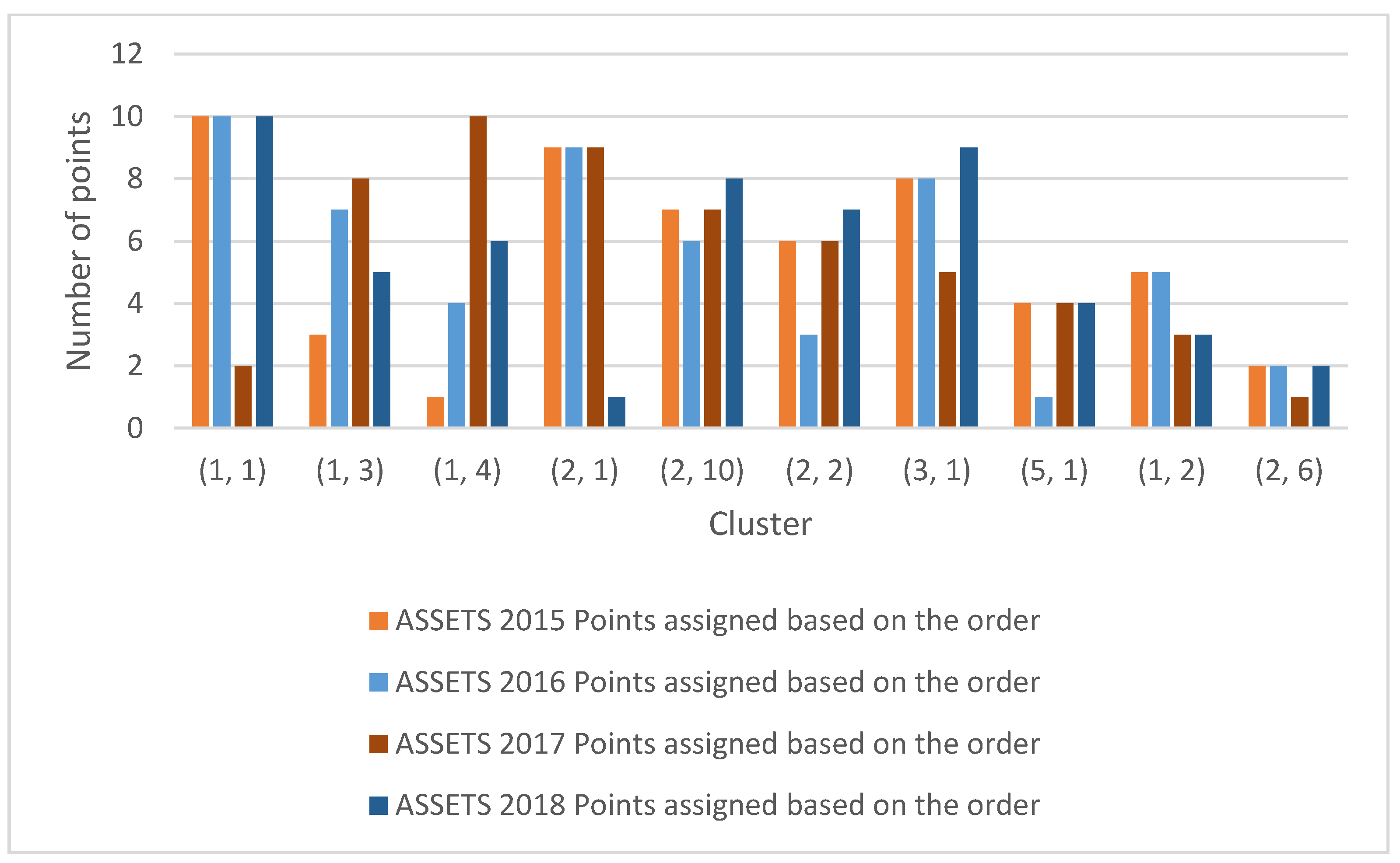
| Assets 2015 | Assets 2016 | Assets 2017 | Assets 2018 | ||||||||
|---|---|---|---|---|---|---|---|---|---|---|---|
| Clusters | Sum of Points Based on the Order | Points Assigned Based on the Order | Clusters | Sum of Points Based on the Order | Points Assigned Based on the Order | Clusters | Sum of Points Based on the Order | Points Assigned Based on the Order | Clusters | Sum of Points Based on the Order | Points Assigned Based on the Order |
| (1, 1) | 1 | 10 | (1, 1) | 1 | 10 | (1, 10) | 9 | 2 | (1, 1) | 1 | 10 |
| (1, 3) | 8 | 3 | (1, 10) | 4 | 7 | (2, 10) | 3 | 8 | (1, 10) | 6 | 5 |
| (1, 4) | 10 | 1 | (1, 2) | 7 | 4 | (10, 10) | 1 | 10 | (1, 3) | 5 | 6 |
| (2, 1) | 2 | 9 | (1, 3) | 2 | 9 | (9, 10) | 2 | 9 | (2, 2) | 10 | 1 |
| (2, 10) | 4 | 7 | (1, 4) | 5 | 6 | (8, 10) | 4 | 7 | (3, 1) | 3 | 8 |
| (2, 2) | 5 | 6 | (1, 5) | 8 | 3 | (3, 10) | 5 | 6 | (5, 1) | 4 | 7 |
| (3, 1) | 3 | 8 | (2, 1) | 3 | 8 | (10, 9) | 6 | 5 | (1, 2) | 2 | 9 |
| (5, 1) | 7 | 4 | (2, 3) | 10 | 1 | (1, 8) | 7 | 4 | (4, 2) | 7 | 4 |
| (1, 2) | 6 | 5 | (3, 2) | 6 | 5 | (8, 8) | 8 | 3 | (1, 9) | 8 | 3 |
| (2, 6) | 9 | 2 | (3, 3) | 9 | 2 | (1, 9) | 10 | 1 | (6, 2) | 9 | 2 |
| Fixed Assets 2015 | Fixed Assets 2016 | Fixed Assets 2017 | Fixed Assets 2018 | ||||||||
|---|---|---|---|---|---|---|---|---|---|---|---|
| Clusters | Sum of Points Based on the Order | Points Assigned Based on the Order | Clusters | Sum of Points Based on the Order | Points Assigned Based on the Order | Clusters | Sum of Points Based on the Order | Points Assigned Based on the Order | Clusters | Sum of Points Based on the Order | Points Assigned Based on the Order |
| (1, 1) | 1 | 10 | (1, 11) | 1 | 10 | (1, 8) | 9 | 2 | (1, 1) | 1 | 10 |
| (1, 3) | 5 | 6 | (1, 2) | 9 | 2 | (10, 10) | 1 | 10 | (1, 3) | 5 | 6 |
| (2, 1) | 2 | 9 | (1, 3) | 2 | 9 | (3, 10) | 5 | 6 | (3, 1) | 4 | 7 |
| (2, 10) | 9 | 2 | (1, 4) | 3 | 8 | (8, 10) | 3 | 8 | (5, 1) | 3 | 8 |
| (2, 2) | 8 | 3 | (1, 5) | 8 | 3 | (8, 8) | 7 | 4 | (1, 2) | 2 | 9 |
| (2, 6) | 7 | 4 | (2, 1) | 4 | 7 | (8, 9) | 6 | 5 | (4, 2) | 6 | 5 |
| (3, 1) | 3 | 8 | (2, 3) | 10 | 1 | (9, 10) | 2 | 9 | (6, 2) | 7 | 4 |
| (5, 1) | 6 | 5 | (3, 1) | 6 | 5 | (2, 10) | 4 | 7 | (5, 13) | 8 | 3 |
| (1, 2) | 4 | 7 | (3, 2) | 5 | 6 | (10, 9) | 8 | 3 | (1, 5) | 9 | 2 |
| (1, 4) | 10 | 1 | (3, 3) | 7 | 4 | (9, 7) | 10 | 1 | (1, 10) | 10 | 1 |
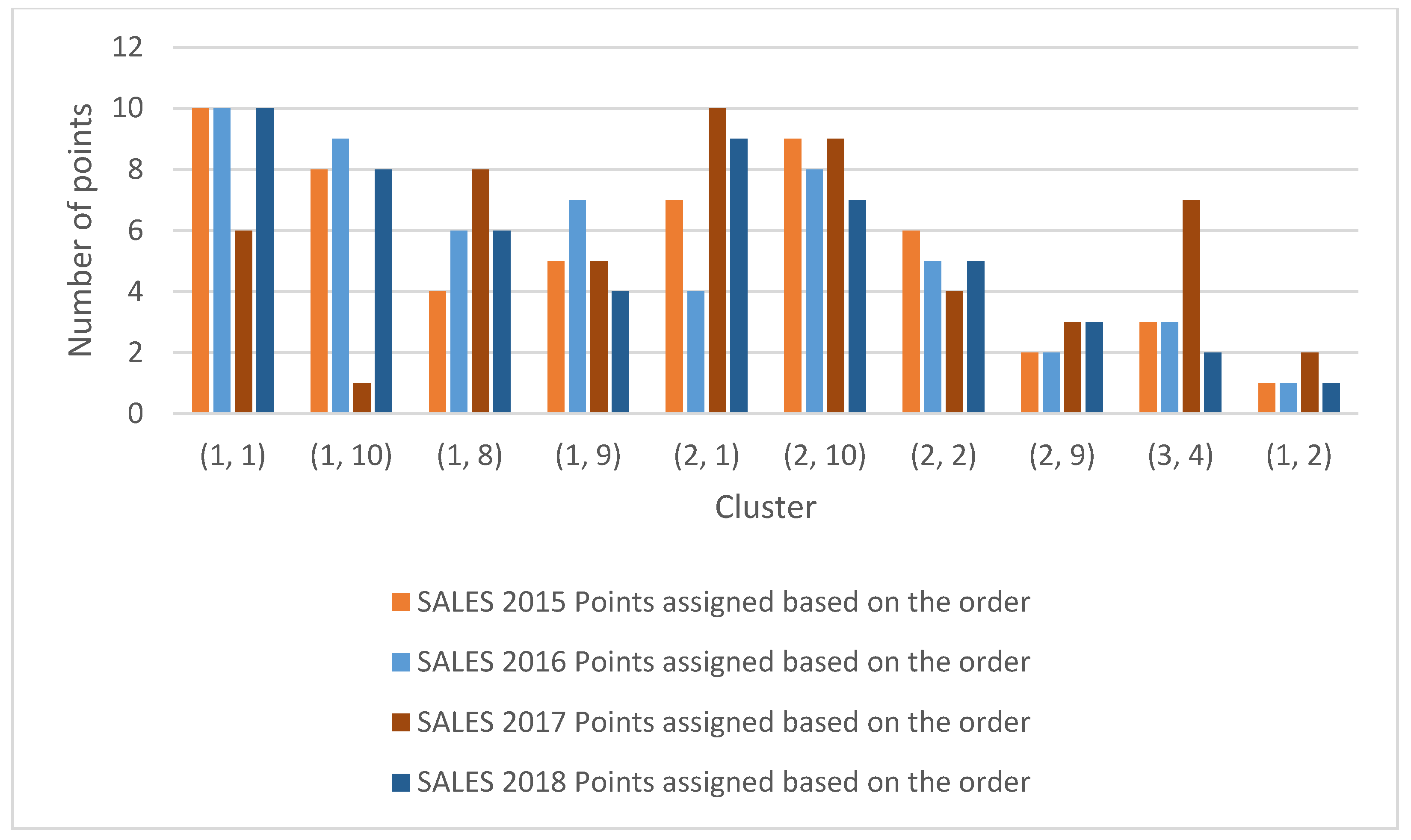
| Sales 2015 | Sales 2016 | Sales 2017 | Sales 2018 | ||||||||
|---|---|---|---|---|---|---|---|---|---|---|---|
| Clusters | Sum of Points Based on the Order | Points Assigned Based on the Order | Clusters | Sum of Points Based on the Order | Points Assigned Based on the Order | Clusters | Sum of Points Based on the Order | Points Assigned Based on the Order | Clusters | Sum of Points Based on the Order | Points Assigned Based on the Order |
| (1, 1) | l | 10 | (l, 1) | l | 10 | (1, 10) | 5 | 6 | (l, l) | l | |
| (1, 10) | 3 | 8 | (1, 10) | 2 | 9 | (1, 7) | 10 | 1 | (1, 10) | 3 | |
| (l, S) | 7 | 4 | (l, 2) | 5 | 6 | (l, S) | 3 | 8 | (l, 9) | 5 | |
| (1, 9) | 6 | 5 | (1, 3) | 4 | 7 | (1, 9) | 6 | 5 | (2, 2) | 7 | |
| (2, 1) | 4 | 7 | (1, 9) | 7 | 4 | (10, 10) | 1 | 10 | (3, 1) | 2 | |
| (2, 10) | 2 | 9 | (2, 1) | 3 | 8 | (10, 9) | 2 | 9 | (1, 2) | 4 | |
| (2, 2) | 5 | 6 | (2, 3) | 6 | 5 | (2, 10) | 7 | 4 | (1, 3) | 6 | |
| (2, 9) | 9 | 2 | (2, 4) | 9 | 2 | (2, 6) | 8 | 3 | (3, 4) | 8 | |
| (3, 4) | 8 | 3 | (2, 2) | 8 | 3 | (9, 10) | 4 | 7 | (3, 10) | 9 | |
| (1, 2) | 10 | 1 | (1, 8) | 10 | 1 | (6, 10) | 9 | 2 | (6, 1) | 10 | |
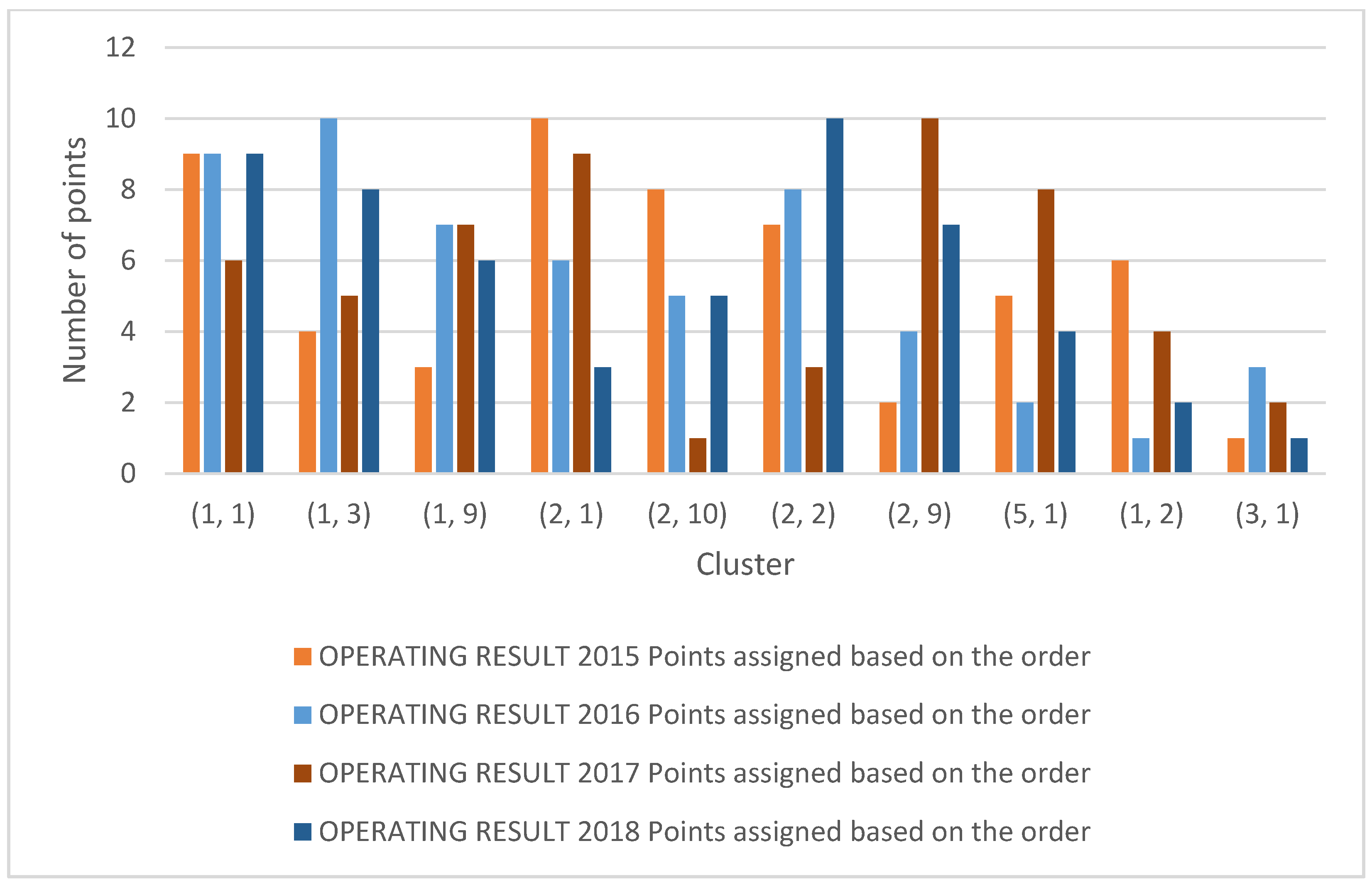
| Operating Results 2015 | Operating Results 2016 | Operating Results 2017 | Operating Results 2018 | ||||||||
|---|---|---|---|---|---|---|---|---|---|---|---|
| Clusters | Sum of Points Based on the Order | Points Assigned Based on the Order | Clusters | Sum of Points Based on the Order | Points Assigned Based on the Order | Clusters | Sum of Points Based on the Order | Points Assigned Based on the Order | Clusters | Sum of Points Based on the Order | Points Assigned Based on the Order |
| (1, 1) | 2 | 9 | (1, 10) | 2 | 9 | (1, 10) | 5 | 6 | (1, 1) | 2 | 9 |
| (1, 3) | 7 | 4 | (1, 2) | 1 | 10 | (1, S) | 6 | 5 | (1, 10) | 3 | 8 |
| (1, 9) | 8 | 3 | (1, 3) | 4 | 7 | (1, 9) | 4 | 7 | (1, 9) | 5 | 6 |
| (2, 1) | 1 | 10 | (1, 5) | 5 | 6 | (10, 10) | 2 | 9 | (2, 9) | 8 | 3 |
| (2, 10) | 3 | 8 | (1, 9) | 6 | 5 | (3, 10) | 10 | 1 | (5, 1) | 6 | 5 |
| (2, 2) | 4 | 7 | (2, 1) | 3 | 8 | (8, 9) | 8 | 3 | (1, 2) | 1 | 10 |
| (2, 9) | 9 | 2 | (2, 2) | 7 | 4 | (9, 10) | 1 | 10 | (3, 1) | 4 | 7 |
| (5, 1) | 6 | 5 | (2, 3) | 9 | 2 | (2, 10) | 3 | 8 | (4, 2) | 7 | 4 |
| (1, 2) | 5 | 6 | (2, 4) | 10 | 1 | (10, 9) | 7 | 4 | (5, 3) | 9 | 2 |
| (3, 1) | 10 | 1 | (3, 1) | 8 | 3 | (2, 6) | 9 | 2 | (2, 2) | 10 | 1 |
| Assets | Fixed Assets | Sales | Operating results | ||||
|---|---|---|---|---|---|---|---|
| Cluster | Points in Total | Cluster | Points in Total | Cluster | Points in Total | Cluster | Points in Total |
| (l, l) | 30 | (l, l) | 30 | (1, 10) | 31 | (l, 2) | 26 |
| (l, 2) | 18 | (l, 3) | 21 | (l, l) | 30 | (l, 10) | 23 |
| (1, 3) | 18 | (3, I) | 20 | (l, 9) | 20 | (1, 9) | 21 |
| (2, 1) | 17 | (1, 2) | 18 | (2, 1) | 15 | (2, 1) | 18 |
| (3, 1) | 16 | (2, l) | 16 | (1, 2) | 14 | (l, 1) | 18 |
| (2, 10) | 15 | (5, 1) | 13 | (2, 2) | 13 | (2, 10) | 16 |
| (1, 10) | 14 | (10, 10) | 10 | (1, S) | 13 | (2, 2) | 12 |
| (5, 1) | 11 | (1, 4) | 9 | (2, 10) | 13 | (3, 1) | 11 |
| (10, 10) | 10 | (2, 10) | 9 | (1, 3) | 12 | (1, 3) | 11 |
| (9, 10) | 9 | (9, 10) | 9 | (10, 10) | 10 | (5, 1) | 10 |
| (8, 10) | 7 | (8, 10) | 8 | (10, 9) | 9 | (9, 10) | 10 |
| (1, 4) | 7 | (3, 2) | 6 | (3, 1) | 9 | (10, 10) | 9 |
| (2, 2) | 7 | (3, 10) | 6 | (9, 10) | 7 | (1, 5) | 6 |
| (3, 10) | 6 | (1, 5) | 5 | (3, 4) | 6 | (1, 8) | 5 |
| (3, 2) | 5 | (4, 2) | 5 | (2, 3) | 5 | (2, 9) | 5 |
| (10, 9) | 5 | (8, 9) | 5 | (2, 6) | 3 | (4, 2) | 4 |
| (1, S) | 4 | (6, 2) | 4 | (3, 10) | 2 | (10, 9) | 4 |
| (4, 2) | 4 | (3, 3) | 4 | (2, 9) | 2 | (8, 9) | 3 |
| (l, 9) | 4 | (2, 6) | 4 | (2, 4) | 2 | (5, 3) | 2 |
| (8, 8) | 3 | (8, 8) | 4 | (6, 10) | 2 | (2, 6) | 2 |
| (1, 5) | 3 | (2, 2) | 3 | (6, l) | 1 | (2, 3) | 2 |
| (3, 3) | 2 | (5, 3) | 3 | (l, 7) | 1 | (2, 4) | 1 |
| (2, 6) | 2 | (10, 9) | 3 | (3, 10) | 1 | ||
| (2, 6) | 2 | (1, 8) | 2 | ||||
| (2, 3) | 1 | (9, 7) | 1 | ||||
| (1, 10) | 1 | ||||||
| (2, 3) | 1 | ||||||
| Clusters | Sum of Points |
|---|---|
| (1, 1) | 108 |
| (1, 2) | 76 |
| (1, 10) | 69 |
| (2, 1) | 66 |
| (1, 3) | 62 |
| (3, 1) | 56 |
| (2, 10) | 53 |
| (1, 9) | 45 |
| (10, 10) | 39 |
| (9, 10) | 35 |
| 2015 | 2016 | 2017 | 2018 |
|---|---|---|---|
| 70,994,234 | 70,994,234 | 70,994,234 | 70,994,234 |
| 25,663,135 | 25,663,135 | 5886 | 25,663,135 |
| 5886 | 5886 | 47,114,983 | 5886 |
| 47,114,983 | 28,196,678 | 60,193,531 | |
| 28,196,678 | 28,196,678 |
| 2015 | 2016 | 2017 | 2018 | |
|---|---|---|---|---|
| Return on assets | −1.46 | −2.89 | −1.62 | −0.81 |
| Return on equity | −1.94 | −3.78 | −2.01 | −0.99 |
| Return on sales | −15.88 | −31.55 | −15.84 | −8.17 |
| Current ratio | 0.73 | 0.86 | 1.05 | 1.09 |
| Quick ratio | 0.63 | 0.8 | 0.93 | 0.99 |
| Cash position ratio | 0.11 | 0.48 | 0.54 | 0.56 |
| Return on assets | 3959.81 | 3990.52 | 3560.83 | 3687.19 |
| Accounts receivable turnover | 184.38 | 103.08 | 87.29 | 106.94 |
| Payables turnover ratio | 264.59 | 362.26 | 238.77 | 258.63 |
| Inventory turnover | 39.14 | 22.57 | 28.34 | 25.93 |
| Debt ratio | 22.82 | 23.43 | 19.23 | 18.08 |
| Debt-to-equity | 30.33 | 30.69 | 23.88 | 22.15 |
| Financial leverage | 1.33 | 1.31 | 1.24 | 1.23 |
| EBITDA | 3,111,929,000 | 1,813,509,000 | 2,939,349,000 | 3,642,561,000 |
| Liability turnover ratio | 496.94 | 666.49 | 502.5 | 540.72 |
| Debtor days ratio | 199.79 | 113.14 | 92.96 | 108.76 |
| Debt coverage ratio | 24.75 | 23.67 | 19.46 | 18.38 |
| Financial debt coverage ratio | 18.22 | 12.79 | 24.2 | 27.92 |
| Fixed asset coverage ratio | 0.93 | 0.94 | 0.96 | 0.98 |
| Bank indebtedness | 7.49 | 4.47 | 1.75 | 0.9 |
| Financial ratio | 0.75 | 0.76 | 0.81 | 0.82 |
| Contribution margin | −76.75 | −85.86 | −85.34 | −117.38 |
| Contribution margin break−even point | 146.80 | 166.71 | 213.53 | |
| Wages/Sales | 135.08 | 138.78 | 141.96 | 162.55 |
| Wages/Added value | −95.06 | −116.23 | −171.06 | −118.28 |
| Cost efficiency ratio | −3.4 | −3.93 | −2.22 | −0.96 |
| Return on investment | 4.16 | 3 | 4.66 | 5.05 |
| 2015 | 2016 | 2017 | 2018 | |
|---|---|---|---|---|
| Return on assets | 1.56 | 2.32 | 2.34 | 1.85 |
| Return on equity | 2.05 | 2.91 | 2.89 | 2.27 |
| Return on sales | 7.11 | 10.44 | 10.22 | 7.89 |
| Current ratio | 0.81 | 0.71 | 0.92 | 1.04 |
| Quick ratio | 0.77 | 0.67 | 0.85 | 0.97 |
| Cash position ratio | 0.66 | 0.56 | 0.65 | 0.78 |
| Return on assets | 1663.57 | 1641.74 | 1589.94 | 1553.53 |
| Accounts receivable turnover | 25.68 | 19.22 | 31.89 | 22.98 |
| Payables turnover ratio | 230.8 | 201.58 | 172.53 | 151.23 |
| Inventory turnover | 8.16 | 9.44 | 11.36 | 10.6 |
| Debt ratio | 23.43 | 19.27 | 18.12 | 17.46 |
| Debt-to-equity | 30.93 | 24.18 | 22.37 | 21.42 |
| Financial leverage | 1.32 | 1.25 | 1.23 | 1.23 |
| EBITDA | 4,970,710,000 | 4,883,945,000 | 5,803,489,000 | 5,598,106,000 |
| Liability turnover ratio | 356.36 | 305.09 | 278.1 | 263.04 |
| Debtor days ratio | 27.72 | 21.37 | 36.16 | 28.86 |
| Debt coverage ratio | 24.27 | 20.28 | 19.01 | 18.52 |
| Financial debt coverage ratio | 22.51 | 33.79 | 35.82 | 34.21 |
| Fixed asset coverage ratio | 0.95 | 0.94 | 0.98 | 0.99 |
| Bank indebtedness | 1.28 | 0 | 0 | 0 |
| Financial ratio | 0.76 | 0.8 | 0.81 | 0.81 |
| Contribution margin | 48.29 | 46.81 | 47.45 | 46.61 |
| Contribution margin break-even point | 38.75 | 60.45 | 65.18 | 63.90 |
| Wages/Sales | 36.05 | 37.6 | 37.79 | 38.51 |
| Wages/Added value | 54.99 | 63.63 | 61.02 | 62.32 |
| Cost efficiency ratio | 6.96 | 8.03 | 8.74 | 6.5 |
| Return on investment | 5.27 | 6.51 | 6.49 | 5.97 |
Publisher’s Note: MDPI stays neutral with regard to jurisdictional claims in published maps and institutional affiliations. |
© 2021 by the author. Licensee MDPI, Basel, Switzerland. This article is an open access article distributed under the terms and conditions of the Creative Commons Attribution (CC BY) license (https://creativecommons.org/licenses/by/4.0/).
Share and Cite
Kalinová, E. Artificial Intelligence for Cluster Analysis: Case Study of Transport Companies in Czech Republic. J. Risk Financial Manag. 2021, 14, 411. https://doi.org/10.3390/jrfm14090411
Kalinová E. Artificial Intelligence for Cluster Analysis: Case Study of Transport Companies in Czech Republic. Journal of Risk and Financial Management. 2021; 14(9):411. https://doi.org/10.3390/jrfm14090411
Chicago/Turabian StyleKalinová, Eva. 2021. "Artificial Intelligence for Cluster Analysis: Case Study of Transport Companies in Czech Republic" Journal of Risk and Financial Management 14, no. 9: 411. https://doi.org/10.3390/jrfm14090411
APA StyleKalinová, E. (2021). Artificial Intelligence for Cluster Analysis: Case Study of Transport Companies in Czech Republic. Journal of Risk and Financial Management, 14(9), 411. https://doi.org/10.3390/jrfm14090411