Article

Testing Housing Markets for Episodes of Exuberance: Evidence from Different Polish Cities

by
Janusz Sobieraj
1 and
Dominik Metelski
2,*
1
Department of Building Engineering, Warsaw University of Technology, 00-637 Warsaw, Poland
2
Faculty of Economics and Management Sciences, University of Granada, 18071 Granada, Spain
*
Author to whom correspondence should be addressed.
J. Risk Financial Manag. 2021, 14(9), 412; https://doi.org/10.3390/jrfm14090412
Submission received: 30 July 2021 / Revised: 26 August 2021 / Accepted: 28 August 2021 / Published: 1 September 2021
(This article belongs to the Section Applied Economics and Finance)

Abstract

:
In the study we use the right-tail unit root test to analyse the presence of mild explosive dynamics (exuberance) in housing prices of the 17 largest Polish cities in the period 2006–2021 (for quarterly data). In terms of real prices from the secondary market, we were able to demonstrate the existence of episodes of mild explosive dynamics for 13 of the 17 cities studied. When we changed the context of the study and performed the same tests for the price-to-income ratio, we found that episodes of price exuberance could be indicated only in the case of two cities. The overall conclusion is that rising average incomes tend to mitigate the explosive dynamics and change the context in which the whole issue of housing bubbles is viewed. The answer to the question of whether there is indeed already a situation of price bubbles in local housing markets in Poland is of course crucial for those interested in buying or selling a housing unit (i.e., the participants of this market), but it must also remain important for the monetary authorities implementing monetary and macroprudential policies in Poland.

1. Introduction

Poland is currently experiencing the second fastest increase in housing prices in Europe (after Luxembourg). At least, this is according to the data published by Eurostat (Eurostat 2021). Taking the average of transaction prices on the secondary market of 10 Polish cities published quarterly by the National Bank of Poland (NBP 2021), the rates of increase in 2018 and 2019 were in double digits (11.8% and 14.5%, respectively) (NBP 2021). In 2020, the rate of increase was already slightly lower, although 8% growth still seems impressive for the period of uncertainty caused by the coronavirus pandemic. So far, 2021 has brought a further continuation and even some acceleration of the strong trend that has been going on for several years (prices rose by 3.65% in the first quarter of 2021 alone) (NBP 2021). From quarter to quarter, real estate prices are marking new all-time highs. Undoubtedly, the rise in property values, caused across Europe by low interest rates and high inflation, is being amplified in Poland by rising housing prices catching up with rising wages. In view of such sharp increases, it is worth asking whether the current market situation is not actually the formation of a price bubble.
It is worth noting that previous evidence shows that loose monetary policy (maintaining low interest rates) undoubtedly favours the formation of bubbles in the long run (Balcerzak 2009; Ciżkowicz and Rzońca 2010; Siwiński 2011; Flotyński 2020). The effects of loose monetary policy are discussed in the studies of Woźniak and Winiecki (2013), Winiecki (2013) and Flotyński (2020). In most cases, low interest rates support the economy only in the short term, while in the long term they prove to be an economic policy mistake and encourage the accumulation of crisis-like developments (Flotyński 2020), for example by leading to a situation of excessive boom in the housing market (Siwiński 2011). It should also be taken into account that the structure of housing demand itself has changed in recent years, in the sense that the value of housing purchases for cash, i.e., without the use of mortgage loans, has increased significantly (Czerniak and Kawalec 2020). This in turn implies that there is now mainly an inflow of portfolio investment into the Polish housing market (in line with speculative demand), which is likely the effect of very low rates of return on alternative forms of capital allocation, such as bank deposits, stock market investments or retail bonds. Czerniak and Kawalec (2020) argue that this situation usually occurs in the declining phases of the housing market boom. According to them, in the early stages of the upward trend in housing markets, purchases are mainly financed by mortgages. In the first half of 2019 alone, the value of cash purchases of residential real estate reached PLN 7.5 billion, which represents a 90% increase compared to the same period in 2015 and 65% more than the value of mortgage demand (excluding own contribution) in the first half of 2019 (NBP 2019; Czerniak and Kawalec 2020). This is hardly surprising given the influx of portfolio investors, as interest rates are close to zero while rates of return (from housing purchases) are either in double digits or near double digits (8% p.a. in 2020). However, it should be borne in mind that portfolio investments are typically speculative in nature, i.e., short-term in nature and aimed at quick returns. The answer to the question of whether there is indeed already a situation of price bubbles on local housing markets in Poland is, of course, crucial for those interested in buying or selling a housing unit (i.e., the participants of this market), but it must also remain important for monetary authorities implementing monetary and macroprudential policies in Poland. A possible collapse of prices in the housing market may lead to sharp economic fluctuations, something that the Polish monetary authorities should be wary of and therefore conduct their monetary policy in such a way as to prevent such a situation (Siwiński 2011; Flotyński 2020). In other words, the NBP should monitor the housing market and take preventive measures against the accumulation of macroeconomic imbalances and the occurrence of sharp economic fluctuations (i.e., preventive measures) that could be caused by a collapse (possible turbulence) in the housing market.
It is worth explaining at this point what a price bubble is in general and how it is defined and presented in the literature. A speculative bubble is a process of unsustainable decline in the market price of a specific asset, subject to a self-perpetuating mechanism (Abolafia and Kilduff 1988). This whole process is coupled with a noticeable market overactivity which is of a transient nature. The very moment of the bursting of an asset bubble is preceded by an intensive boom phase, i.e., a relatively fast rise in prices, which is followed by a meltdown phase, i.e., a sudden collapse of prices (Czerniak and Witkowski 2016). The evolution of this process can be explained by a positive feedback loop mechanism (i.e., the so-called snowball effect) known from the systems theory, which first causes a sharp rise in prices (i.e., reinforces price increases) and then usually leads to an even sharper collapse, introducing a state of disequilibrium, driving the price action out of its equilibrium (Czerniak and Kawalec 2020).
The process of bursting bubbles is accompanied by a decline in wealth of many investors. A speculative bubble is also referred to as a price bubble, speculative balloon, speculative mania, speculative frenzy, “speculative fever”, etc. Typically, housing bubbles occur when property prices rise without any special rational reasons finding their justification in the market, e.g., rising reconstruction values due to material or labour price increases. However, according to Lind (2009), a price bubble should not be defined on a rational–foundational basis, but only in relation to the price action (price evolution) itself. In a nutshell, to identify a bubble in any market, it is enough to indicate periods of rapid increases followed by rapid falls in prices. In contrast, the prospect of assessing valuations through the lens of fundamental analysis, in the context of price discovery alone, should not be considered at all. As Lind (2009) notes, looking at price collapses in terms of fundamental analysis could seem problematic, since the very concept of ‘fundamental analysis’ is an ambiguous and partly discretionary one. Lind (2009) argues that price bubbles usually cannot be explained by a single factor, but are the result of the interaction of many factors. It is however possible to develop whole sets of indicators, although these should only be treated as warning signals. In addition, such a picture can be linked to price evolution, indicating sharp falls in prices after a preceding period of rapid increases—and if such a situation arises, it is reasonable to assume the existence of bubbles. Lind (2009) points to factors such as interest costs relative to household income, supply elasticity, price expectations and credit conditions.
Typically, in a situation of bubble occurrence, psychological factors become dominant, which is based on the expectations of market participants (Czerniak and Kawalec 2020). For example, potential buyers, noticing an established upward trend, and fearing further price increases, are more inclined towards quicker action and decide to make a purchase in order to catch up with further price increases. Bubbles are caused by the overactivity of market participants, which in turn leads to unimaginable increases in asset prices, followed by periods of visible price collapses. The traditional understanding is that housing bubbles occur when housing prices exceed the reconstruction value of a real estate, or in other words the total fair value of all the components required to recreate such real estate in the same location. This in turn is related to the replacement cost or replacement value that an entity would have to pay to replace the housing unit at its face value. Bubble formation occurs when housing owners believe that they can obtain a price that is higher than the fair value (Malkiel 2010). Most often than not, investors are lured into investing at times of bubble formations, which is often irrational and based on pure expectations of a continuation of the prevailing upward trend. Naturally, at some stage of such a rise in prices there must come a point when investors begin to understand the irrationality of the whole situation and they do not expect prices to rise any further, at which point there is a fall in demand and a sudden collapse in prices (Shiller 2003).
Periods of irrational price exuberance in housing markets occur quite frequently. A number of examples of the episodes of price exuberance in housing markets can be found in the paper by Oust and Hrafnkelsson (2017). More than a decade ago, when housing bubbles had burst in many countries, apart from the losses in the real estate sector, it caused turmoil in the whole financial system, and spilled over to other sectors inducing a sharp recession in many countries across the globe. Arguably, there is no need for further evidence demonstrating that housing markets constitute an extremely important element of any economy, and since they are now also highly financialised, they have therefore become an integral part of modern financial markets (Said et al. 2014; Kamiński 2019; Wijburg 2020).
Long-term price increases in housing markets usually lead many participants of these markets to believe that investments in this type of assets are risk-free. Of course, in reality this is not the case, and in certain situations real estate may lose its value in a very dynamic manner. The fact of the matter is that buying property in a bubble price environment involves very high risks, which are often underestimated. The problem is all the more significant because it is not uncommon for a purchasing decision to be accompanied by the launch of a multi-year mortgage financing procedure that can last up to 30 years. The borrower taking out such a mortgage loan over the entire many-year period of its service has to take into account the possibility of the occurrence of a number of recessions, which in turn may worsen his/her financial situation and cause him/her to fail to pay the instalments in a timely manner. If such a situation occurs, the lending institution may foreclose his/her mortgage. This was precisely the situation that caused the subprime crisis in the United States more than a decade ago, when Americans learned the hard way what the bursting of a housing bubble can result in. That crisis was caused by a fall in real estate prices in a heavily financialised housing market, in which purchases of a large percentage of housing were made with the use of mortgage loans, granted to people who did not have sufficient creditworthiness. Nevertheless, the banks were giving them such loans anyway.
The aim of this study is to identify episodes of price exuberance in the housing markets of various Polish cities, relying on two different sets of data, i.e., the real housing prices and the price-to-income ratio. In the study, we rely on quarterly housing price data (from the secondary market) published by the NBP, covering the period from the third quarter of 2006 to the first quarter of 2021. The study will allow us to determine whether we can identify periods of mild explosive dynamics with regards to real housing prices or the price-to-income ratio. Furthermore, our study will help to indicate the existence of bubbles at the regional level, and the research method on which the study is based allows for testing and date-stamping periods of explosiveness (or exuberance) in time series, and provides more accurate results than standard econometric studies based on, for example, the augmented Dickey–Fuller (ADF) tests. Viewed from this perspective, we expect that our study will further add to the abundant practical evidence already existing in the literature in this regard.
Indeed, it is unarguable that housing prices in most Polish cities have recently risen to such an extent that some have referred to it as a nascent bubble, yet this claim remains formally unproven to this day. The hypothesis we put forward in our study can be reduced to postulating that in the case of many Polish cities there can be found episodes of price exuberance (especially in the last 5 years), but given certain foundations and purchasing power parity, the situation may look very different. In other words, looking from the perspective of changes in housing prices, we can expect the occurrence of explosive dynamics, looking through the prism of the generalised sup Augmented Dickey–Fuller supremum augmented Dickey–Fuller (SADF) and generalised sup Augmented Dickey–Fuller (GSADF) research methods, however, should we take into account a much bigger increase in average incomes than in housing prices themselves, most likely, when applying the same method, we will not be able to demonstrate the occurrence of as many episodes of explosiveness as in the case of the change in real housing prices. Our aim is also to present a panel approach, by means of which we will be able to unambiguously assess changes in real prices and the price-to-income ratio for 17 Polish largest cities.
This paper contributes to the global literature by extending the empirical evidence on testing episodes of price exuberance by including the most recent results for local housing markets in Poland. In addition to applying the right-tailed unit root test procedure to recent quarterly data on transactional secondary market housing prices covering 17 major Polish cities, the study shows the practical application of the GSADF panel test to all of these markets. The paper also shows that the same method of assessing housing price action (price trends for raw data) and data reflecting changes in housing prices in relation to changes in the average income of residents in these local markets yield different results.
The structure of the paper is very straightforward. In the following part we review different approaches for studying housing bubbles discussed in the literature. In the subsequent empirical part, we focus on the analytical aspects, methodology, the results and a discussion. The paper ends with the final conclusions.

2. Literature Review

The housing market fulfils an important function in the global economy, and fluctuations in real estate prices translate into the financial health of banks and the financial sector as a whole. Clearly, it is not only the housing market that affects the economy, but economic downturns also have an impact on housing price fluctuations (Quigley 2002). In other words, housing markets and the economy are systems of two-sided interconnectedness. Housing markets affect macroeconomic and financial stability, if only because of the size of these markets and the wealth effect they create1. The perception of growing wealth (affluence) translates into higher levels of confidence and increases household spending. In such a favourable environment, households are more likely to take out loans and increase their consumption, which is associated, of course, with increasing housing prices. As a result, rising housing prices lead to a redistribution of wealth.
Sobieraj (2020) argues that not only is the wealth effect created by the housing bubble superior to that of the stock bubble, but the eventual bursting of the housing bubble may have more dangerous consequences on the overall economy as opposed to the bursting of the stock bubble. Individual consumption is more responsive to changes in housing prices versus changes in stock prices. This is due to the fact that housing-related assets find a much higher representation in total household wealth. Besides, it is important to remember that real estate is used as collateral for a large part of the total mass of other bank loans. Property owners whose prices go up will inherently be inclined to consume more, since their belief about their own wealth is more strongly ingrained in them.
Machaj (2016) points out that the expansion of the mortgage market, facilitated by low interest rates, contributes to the housing bubble. This is because housing is largely financialised through mortgage loans provided by the banking sector and, in addition, this area of financial institutions’ activity accounts for a large share of their total activity. What is more, there is an ever-increasing share of debt instruments used for financing housing purchases (Sobieraj 2020). It is also important to note that such purchases are most often financed with the use of financial leverage, which in this category of purchases is incomparably higher as opposed to other asset classes. This causes the amounts of loans given by banks to be very high when considering their face value.
By the same token, the housing market is extremely sensitive to price fluctuations. A growing real estate market is accompanied by an increase in the share of purchased housing financed by mortgage loans; this is because in a growing real estate market financial institutions are typically more eager to facilitate access to housing loans. Such was the case, for example, in the US during the period preceding the subprime crisis.
Xiao and Devaney (2016) point to the relationship between prices and lending and the assumption of consumer rationality in this regard, which determines the prevailing theoretical models of housing prices and borrowing. The authors stress that local markets are structurally different and the specifications of every estimated housing market model should vary across different regions. Moreover, Xiao and Devaney (2016) investigated differences in the price–credit relationship for different regions of the UK in an attempt to capture asymmetric market behaviour and turning points based on Markov switching regimes. The results of their study show that credit abundance had a large impact on housing prices. More specifically, there may be some positive feedback effects in housing markets following previous price movements. Therefore, the credit effect and the feedback loop effect have to be seen in terms of the system dynamics. Additionally, Xiao and Devaney (2016) argue that market turning points and bubble probabilities can be distinguished with the use of a discrete Kalman filter. Xiao and Devaney (2016) point to the relationship between the amount of mortgage interest relative to the risk-free rates and every household individual mortgage situation, or in other words, the association between the amount of collateralised credit and individual financial standing of the mortgage borrower. Typically, bubbles form in environments where housing buyers misinterpret the base price due to insufficient information. In this context, market efficiency expresses the extent to which market prices reflect all available, relevant information. If we assume that housing markets are efficient, it would mean that we take for granted that all information is already factored into prices, which we know is not the case. The inefficiency of housing markets has been confirmed in studies using a framework that considers both temporal and spatial dimensions (Tirtiroǧlu 1992). However, in efficient financial markets, over time prices revert to their fundamental levels.
The fact of the matter is that prices in real estate markets can remain above the baseline for a relatively long time, or at least as long as optimistic investors remain in this market and there is an adequate financing in place. This situation can also be influenced by construction delays insofar as new housing is concerned, thereby controlling supply and particularly fostering price increases and the formation of bubbles. Eventually, however, price increases become very noticeable and a feedback-loop mechanism kicks in, bringing valuations to more realistic levels.
Zhao et al. (2017) argue that a comprehensive analysis of the relationship between housing market and finance makes it easier to predict an upcoming burst in a bubble economy. They suggest that a financial crisis often emerges from a weak financial system which is too closely linked to the country’s housing sector. These linkages allow housing crises to transform into financial crises. In turn, these financial crises balloon into macroeconomic crises. Moreover, Zhao et al. (2017) explain the formation of bubbles by the fact that nominal asset prices are misaligned with underlying values and short-term incentives for economic agents differ from long-term benefits.
De Bandt et al. (2010) point out that the natural state of housing markets is a long-term upward move which is largely attributable to some inconsistencies in a technological progress between housing and other sectors of the economy. Paries and Notarpietro (2008) attribute the reasons for the upward trend in real house prices over the last few decades to technological progress in the housing sector, partly also to monetary factors (around 20 per cent). Brunnermeier and Julliard (2008) argue that there is a certain persistency in the upward tendency of prices in the housing market, which encourages an increase in transaction volume and props up higher valuations. Previous experiences show that booms in this market may be sustained over many years. Iacoviello (2010) accentuated the importance of the housing sector to the overall economy. He indicated a number of stylised facts about the importance of housing to macroeconomic performance. He pointed to the growing importance of financial intermediation, the role of economic policy and labour markets, among other things.
However, it cannot be ignored that the interconnectedness between housing and financial markets has become increasingly strong in recent years and the housing markets themselves have therefore to a large extent become financialised in their nature (Said et al. 2014; Kamiński 2019; Wijburg 2020). Wijburg (2020) notices that housing financialisation, or the increased dominance of financial markets in the housing sector, has not stopped in the wake of the crisis. Rather, it has reinforced and rescaled itself, expanding into new market segments and urban territories. This obviously increases the risk of future financial crises as a result of housing bubbles (Leijten and de Bel 2020).
It should be noted that mortgages created for banks through the lending channel are reflected on banks’ balance sheets, which always carries certain risks (Allen and Carletti 2013; Zhang and Bezemer 2014). Let us assume for the sake of argument that housing prices would suddenly collapse. Then, when preparing the next balance sheet, revaluations would have to be made in accordance with certain accounting standards, which in turn would reveal certain capital shortfalls for the banks. This, in turn, would entail a systemic risk that could spread to other sectors of the economy through the credit channel. Hence the need for strong risk-based capital requirements for mortgage loans held in the portfolios of financial institutions (Calem and LaCour-Little 2004). The whole economy is a system of interconnected vessels, and a lack of liquidity in the system can affect many different sectors. When a housing bubble bursts, the collapse of the financial system is reflected not only in the property sector, but usually also in other sectors (Elliott and Neil Baily 2009). In general, the lack of liquidity in the banking system results in limited lending activities, affecting the whole economy, and particularly credit-driven economies (Vogiazas and Alexiou 2017).
Housing markets represent an important component of local economies, and history shows that they play an important part in the creation of financial sector bubbles. This is largely due to the fact that any wealth that is created from an increase in housing prices is many times greater than the wealth effect from an increase in the prices of other assets, and consequently a collapse in the housing market results in more destructive effects for the economy as a whole as opposed to a similar collapse in other asset markets, such as stock markets, for example. This is precisely why the operations that take place in this market should be carefully monitored by governments, in terms of the financial stability of the whole system and systemic risk (Czerniak and Kawalec 2020). It is worth noting that housing frictions are becoming more frequently incorporated into different economic models, such as the dynamic stochastic general equilibrium (DSGE) models (Paries and Notarpietro 2008; Iacoviello 2010; Iacoviello and Neri 2010; Sobieraj and Metelski 2021), accounting for important characteristics of the housing market. Although DSGE models are not a tool for detecting bubbles, they do a good job of explaining their causes (which is why they are worth mentioning). For example, Ng (2015) estimated a DSGE model to study the sources of housing market dynamics in China and found that monetary shocks explain 12–32% of the variance in housing prices. Rubio and Carrasco-Gallego (2016) took a DSGE model and showed how different shocks contributed to the increase in housing prices in the context of European countries. As far as their study is concerned, the DSGE model helped to understand the interaction between liquidity and the shocks with housing prices. Moreover, a DSGE model allows characterising conditions for the existence of rational bubbles, taking into account the fundamental value of the underlying assets (Wang and Wen 2012).
In the literature there are many theoretical and empirical studies on housing bubbles. Diba and Grossman (1984, 1988) and Hamilton and Whiteman (1985) tested the existence of rational bubbles by examining the stationarity of asset prices and observable fundamental factors. Ardila et al. (2013) studied the existence of bubbles in the Swiss housing market between 2005 and 2013. To this end, they relied on the log periodic power law (LPPL) model. Their results showed the existence of bubbles in a number of districts of the country. Basco (2014) studied the links between globalisation and the formation of rational bubbles in housing markets. According to him, globalisation has intensified the formation of such bubbles. Basco (2014) has also shown that the probability of a bubble is larger in environments of highly globalised and financialised markets and it increases with the degree of financial development of such markets. Zeren and Ergüzel (2015) studied the occurrence of bubbles in the housing markets of Turkey’s three largest cities, i.e., Istanbul, İzmir and Ankara, between January 2010 and June 2014. More specifically, they based their study on the SADF and GSADF recursive unit root methods developed by Phillips et al. (2011). Their results showed that while above-normal increases (price increases above the average) usually occur in short periods, they are not sustained in the long term. Zeren and Ergüzel (2015) refer to the studied housing markets in the context of the efficient market hypothesis, which in their view finds positive validation, making these markets much more resilient to housing mortgage crises similar to the one from 2008/2009. Their findings demonstrate the stability of the Turkish housing market, which they attribute to the right pricing policy following the crisis.
Caspi (2016) studied the presence of housing bubbles in the Israeli market between 2008 and 2013. For that market, price exuberance seemed to be evidenced by a 10% average real annual growth rate in housing prices in the period under study (around 50% in real terms, with some Israeli regions experiencing an increase of nearly 60%). The author relied on Gordon’s dynamic growth model and on the explosive episodes detection models proposed by Phillips et al. (2011), Phillips et al. (2015b) and Homm and Breitung (2012), which he employed to quality-corrected housing prices data. However, for the Israeli data the null hypothesis of no exuberance failed to be rejected. The results proved robust across different model specifications, i.e., taking into account financial leverage and mortgage rates. Caspi (2016) examined the responsiveness to the selection of the lag length across various model specifications. Ultimately, he came to the conclusion that housing price increases are driven by changes in fundamental factors, i.e., rental rates and interest rates.
Engsted et al. (2016) analysed price exuberance in housing markets in Organisation for Economic Cooperation and Development (OECD) countries over the period 1970–2013 (for quarterly data). To this end, they applied Vector autoregression (VAR) procedures (Engsted and Nielsen 2012) for testing for explosive dynamics and a one-factor, right-tailed unit root test (Phillips et al. 2015a, 2015b) on price-to-rent ratios at the country level. Their results provided evidence of episodes of explosive dynamics in many OECD housing markets. More specifically, their findings supported the hypothesis of price exuberance, i.e., the existence of bubbles in these markets. Martori et al. (2016) took six major metropolitan regions in Spain and analysed the spatial structure of excessive growth in the construction sector between 2001 and 2011. To this end, they used a method known as the Explanatory Spatial Data Analysis (ESDA) and showed that housing bubbles have increased spatial autocorrelation in the period under study, most notably in large Spanish cities such as Madrid and Barcelona. Solak and Kabaday (2016) examined the causes of rising housing prices in Turkey between 1964 and 2014 and found evidence indicating that the driving force behind an increase in housing prices is associated with household real income. Furthermore, they pointed to a positive relationship between prices and demand for housing, as measured by the total number of square metres of sold housing units. This in turn may indicate that housing units may also be viewed as investment goods. More specifically, the authors relied on such research methods as recursive unit root tests, integration tests, which they employed for testing the stationary properties of the time series data.
Xiao and Devaney (2016) studied differences in the price–credit relationship for 12 UK regions. To show asymmetric market behaviour and tipping points they relied on Markov regime switching research method. In this way, they showed that credit abundance plays a role in terms of changing housing prices. The authors also demonstrated a strong positive feedback loop effect resulting from past housing price movements. It appears that a strong positive feedback loop effect arising from past lending activity may also be evident in the credit dynamics. Additionally, the study by Xiao and Devaney (2016) provides evidence showing that market tipping points can be detected with the use of a discrete Kalman filter.
Coskun et al. (2020) sought episodes of price exuberance in Turkish housing market in the period 2007–2014. They captured the determinants of housing prices using the Bounds test as well as other research methods such as Ordinary Least Square (OLS), Fully Modified OLS (FMOLS), Dynamic OLS (DOLS), Kalman filter and AutoRegressive Integrated Moving Average (ARIMA) models, and came to the conclusions that although Turkish housing market was overvalued, there were no signs of a bubble in that market. In the latter case, the aim was to examine whether rising housing prices were justified by fundamentals. The results of the Bound test provided evidence of a long-term cointegration between housing prices indices and housing rentals, construction costs and the real mortgage rates. The Coskun et al.’s (2020) study provides evidence of an overvaluation of the Turkish housing market in the studied periods, although no support was found to support the price exuberance hypothesis. Shi (2017) studied the occurrence of speculative bubbles in the US over a period of almost three decades (1978–2015), and more specifically in national and regional housing markets (21 regions). She proposed a new method for examining exuberance in housing markets in real time, based on screening the fundamentals of housing market valuations against changes in macroeconomic indicators, including employment, changes in population size, interest rates, per capita income, etc. This method eliminates periodically collapsing bubbles in that it significantly reduces the chance of a false positive identification of the episodes of explosiveness, overcoming the shortcomings of other approaches such as those proposed by Phillips et al. (2015a, 2015b). In the case of the US market, Shi (2017) identified one bubble episode throughout the sample period in the national housing market, namely in the early to mid-2000s. On the other hand, at the regional level, she identified two episodes of explosive price dynamics.
Vogiazas and Alexiou (2017) studied the relationship between housing prices and the business cycle in seven advanced OECD economies over the period 2002–2015. Their study relied on the panel research method developed by Phillips et al. (2011, 2015a, 2015b). The panel framework allowed them to identify the determinants of housing prices (i.e., real gross domestic product, bank credit growth, long-term bond yields and real effective exchange rates), while the bubble detection tests provided evidence of the linkage between credit action and the propagation of housing booms. The findings of the study by Vogiazas and Alexiou (2017) may serve as a tool that detects formation of housing bubbles. Escobari et al. (2015) examined the existence of bubbles in 15 US metropolitan areas at the time of the 2008/2009 housing bubble. They proposed a new method (empirical time series test) to identify episodes of exuberance in housing markets. The research method developed by Escobari et al. (2015) identifies explosive dynamics as structural breaks in the difference between appreciation rates of Case-Shiller price levels.
Shi et al. (2016) tested for explosive dynamics in housing price-to-rent ratios in Australian capital cities. To this end, they adopted the Phillips et al.’s (2015a, 2015b) approach, and their results for the period 1995–2015 indicated a varying degree of speculative behaviour in capital cities in the 2000s, before the Global Financial Crisis (GFC) of 2008 engulfed various housing markets. More specifically, the authors provide significant evidence of exuberance in housing prices relative to rents in Sydney. The method developed by Phillips et al. (2015a, 2015b) can be treated as an early warning indicator for detecting housing bubbles in various markets.
Greenaway-McGrevy and Phillips (2016) provide evidence showing price exuberance in the New Zealand housing market in the period of the last two decades. The authors used statistical methods to test for and stamp-date price exuberance in housing (Phillips et al. 2015a, 2015b). They also examined the spillover of the housing bubble from Auckland to other metropolitan centres (the so-called bubble contagion effect to other centres). They argued that expensive nature of New Zealand housing relative to potential rental incomes was the result of some sustained market exuberance that had produced a broad-based housing price bubble over the past decades2. Pedersen and Schütte (2020) applied bootstrap test to examine the existence of housing bubbles in OECD countries, however, they found much weaker evidence for housing bubbles compared to prior evidence. Wei et al. (2020) assessed housing bubbles in 140 US cities by identifying the formation of bubbles and their subsequent bursting between 1989 and 2017. To evaluate regional housing bubbles in the US, the authors employed the generalised supremum augmented Dickey–Fuller (GSADF) test, which is an innovative and powerful method for detecting bubbles. The results of their study allowed them to identify housing bubbles in nearly 30% of studied locations (or, more precisely, in 45 out of 140). They also reached some conclusions of a more evolutionary-structural nature concerning specific regions, which allow for a better understanding of the market dynamics and evolutionary patterns of housing bubbles.
As for the Polish context, there are not many studies dedicated to assessing whether bubbles have occurred in the Polish housing market. The most recent ones include a study by Żelazowski (2018), followed by the work of Czerniak and Kawalec (2020). Regarding the former, Żelazowski (2018) assessed changes in household purchasing power in 17 local housing markets (using quarterly data from 2003 to 2016) based on the GSADF test proposed by Phillips et al. (2011, 2015a, 2015b). According to the test results in Żelazowski’s (2018) study, the bubble phenomenon was experienced in all local housing markets. The author attributed the reason for the occurrence of price bubbles mainly to macroeconomic conditions. Among the cities with exceptionally high price increases in relation to household income, Żelazowski (2018) refers to Białystok, Łódź, Opole and Kielce. Czerniak and Kawalec (2020), in turn, base their study on statistical measures calculated according to the methods developed by Bordo and Jeanne (2002) and Czerniak (2014). Their results suggest the presence of price bubbles in the Polish housing market, especially in the secondary market. More specifically, they indicated episodes of price exuberance in 15 and 17 cities (out of 17 studied), depending on the method used. The authors used quarterly data covering the period from 2006 to 2019. In turn, according to Korzeb (2019), who also studied the presence of bubbles in the Polish housing market, the analysis of two economic indicators, i.e., the ratio of household housing loans to GDP, expressed in growth rates, and housing price growth rates, does not suggest that there is currently a speculative bubble on the Polish housing market. Additionally, Slavata (2018) compared housing prices and its availability (affordability) in Poland, Czech Republic and other EU countries (using July 2018 data), and taking three categories of data (raw data, Price-to-Income, Price-to-Rent), he concluded that housing is much cheaper in Poland than in Czech Republic or in most EU countries. The author also showed valuations and undervaluations of housing units in the studied regions, and as it turns out, Polish houses seem to be much cheaper compared to those of the Czech Republic (the Małopolska region was a single exception).

3. Materials and Methods

3.1. Data Descritpion

While there are many sources of data on housing prices in the Polish primary and secondary housing markets, most of them mainly refer to list prices in several major cities and usually come from the records of a particular broker or developer (Czerniak and Kawalec 2020). The most reliable lists are published quarterly by the Central Statistical Office (GUS) and the National Bank of Poland (NBP). Both the GUS and the NBP collect quarterly data on transaction prices, including prices on the primary and secondary markets. However, Czerniak and Kawalec (2020) point out the superiority of the NBP data, partly due to the fact that their database covers a longer time series, i.e., from the third quarter of 2006 to the most recent quarter; the data are available for 17 voivodship cities. The GUS data, on the other hand, cover only the last 10 years. As Czerniak and Kawalec (2020) correctly note, the data from GUS are therefore unsuitable for studies of price bubbles because they cover too short a period; a much longer data set covering at least a full cycle in the housing market is needed to study episodes of price exuberance. This seems especially important when different time windows are chosen, e.g., 8, 10 or 12 periods, as is the case in this study. Therefore, this study relies on quarterly transaction data on housing prices from the secondary market provided by the National Bank of Poland.
The price-to-income ratio is the relationship between market prices for housing and average wages. Average gross monthly wages for voivodeship cities were taken from the database of Central Statistical Office (GUS). The use of the average price of residential real estate in the calculation of the price-to-income ratio imposes a certain burden on the obtained results. According to the literature, the analysis of price trends in the real estate market using simple measures based on the mean or median does not take into account the changes in the qualitative and quantitative characteristics of traded real estate in subsequent periods (Trojanek 2008; Widłąk 2010; Żelazowski 2018). More effective solutions in this respect are, for example, the hedonic index of housing prices of the National Bank of Poland.
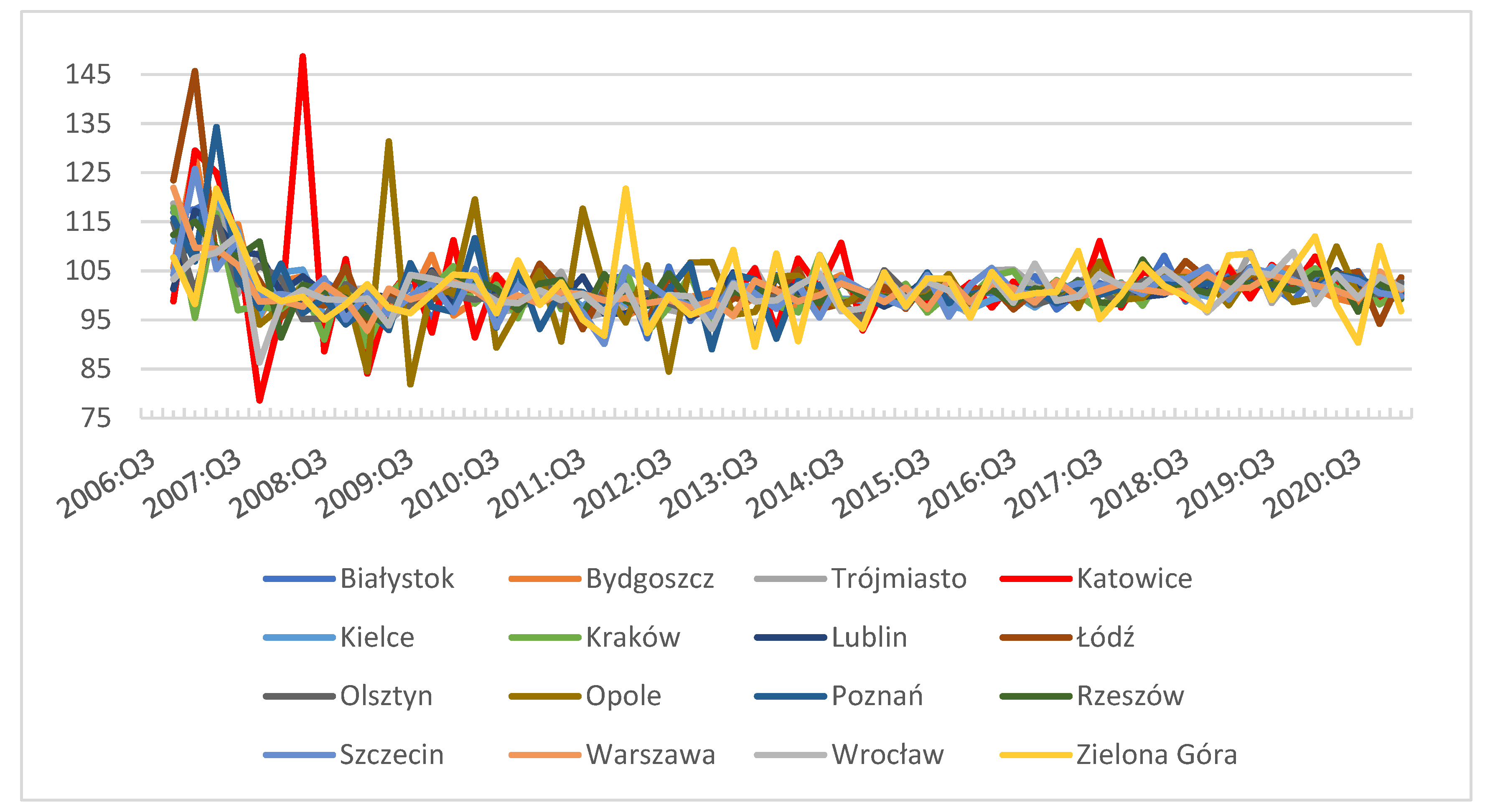
Figure 1 shows that for a number of years (practically for the whole decade), real housing prices in Polish largest cities remained in a sideways trend (apart from 2008 to 2009, when the real estate crisis took place, which initially started in the United States—as a subprime crisis, and then spread around the world), and in the last 5 years, prices broke out of this sideways trend and started a runaway upward move.
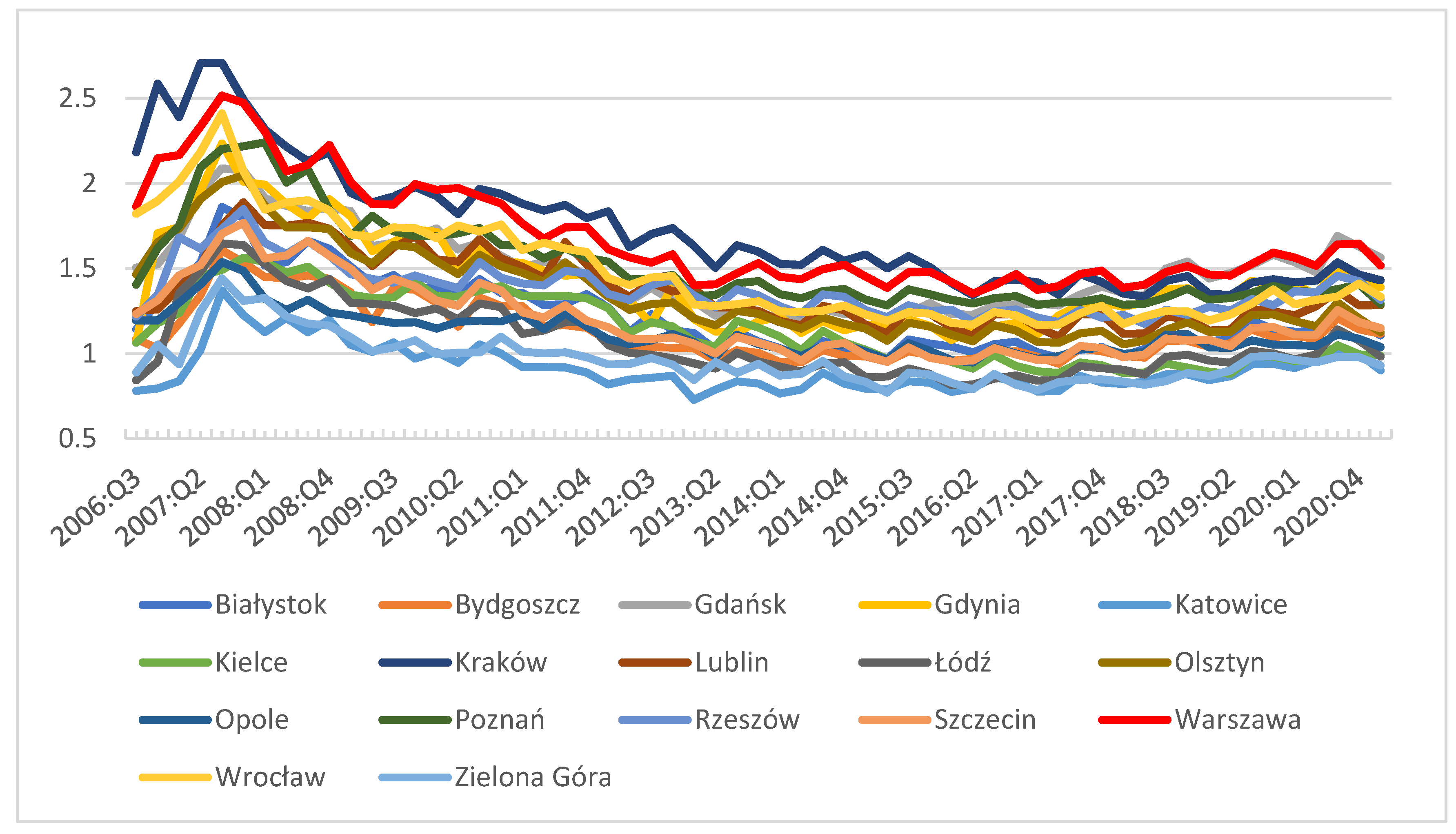
An even better insight can be gained by examining Figure 2 (hedonic price index), which shows quarter-to-quarter (q-o-q) price changes. It shows that, more or less until the fourth quarter of 2015, quarter-on-quarter changes had both large upward and downward swings, i.e., they exhibited a stochastic behaviour. Subsequently, with minor exceptions e.g., Zielona Góra, prices started to rise.
The case of the price-to-income ratio is completely different (see Figure 3). This ratio has been decreasing for a number of years, i.e., from the first quarter of 2008 to the first quarter of 2016. Therefore, it can be observed that the decrease in the price-to-income ratio can be associated with a relatively stable period in terms of changes in real housing prices. Reaching a certain threshold for average income growth at the regional level may have been the catalyst for the start of a mini bull market in housing. Since most asset prices have a tendency to the so-called volatility clustering, the started trend usually lasts for a number of years.
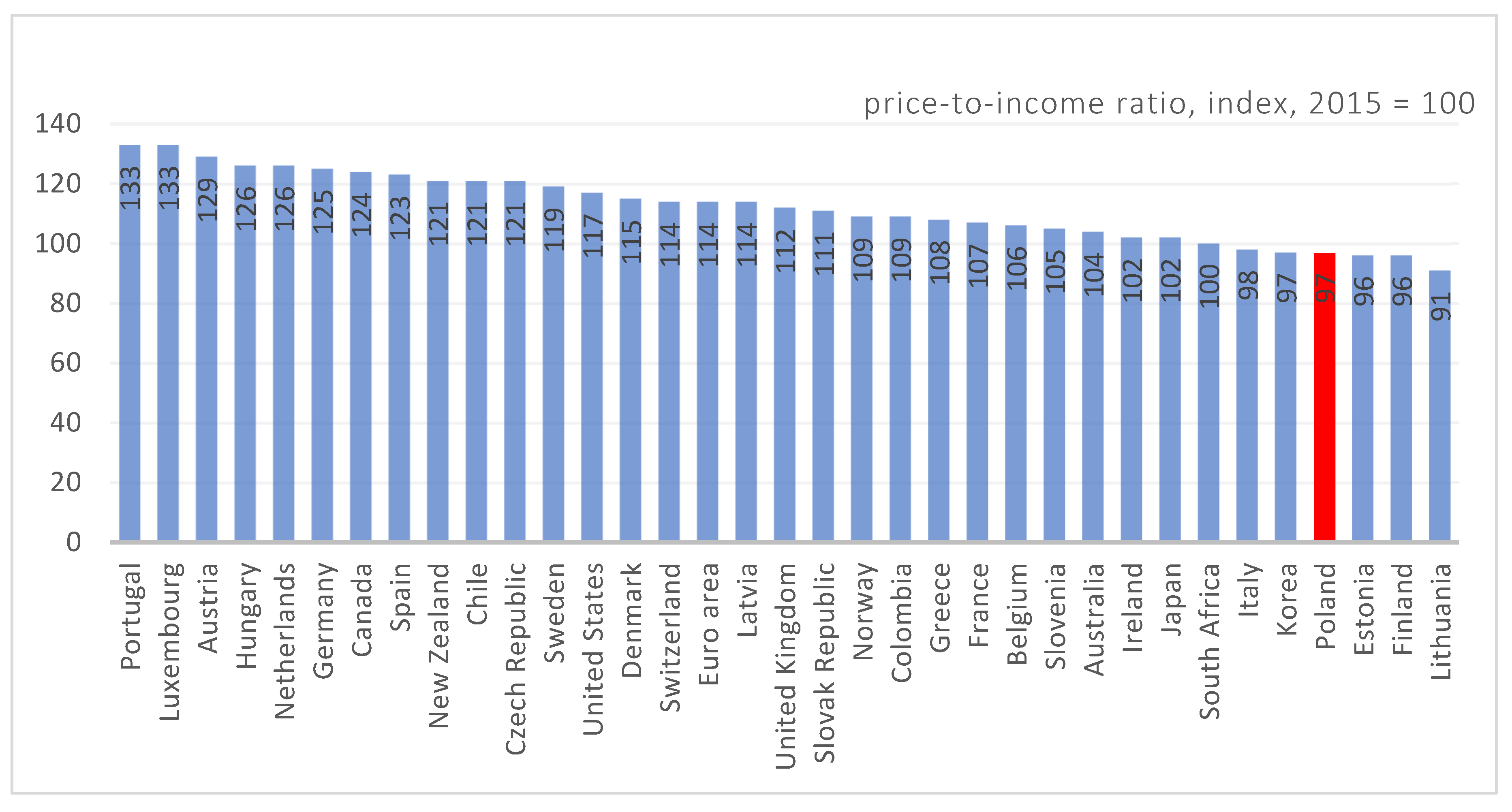
Figure 4 shows that compared to other EU countries, housing prices in Poland still seem to be cheap. The price-to-income ratio by OECD of 97 places has Poland in one of the last positions in Europe (only Estonia, Finland and Lithuania have lower ratios), which shows that housing prices are still relatively cheap compared to other EU countries.

3.2. Different Approaches for Detecting Explosive Dynamics

There are many research methods in the literature for identifying price bubbles; some of them are simple statistical analyses, but there are also a whole range of complex econometric models, including nonparametric models (European Central Bank 2010; Czerniak and Kawalec 2020). Many of these models are used to build so-called early warning systems (EWS) (Dreger and Kholodilin 2013). A complete and effective EWS supports four main functions: Risk Analysis, Monitoring and Warning, Dissemination and Communication, and Responsiveness. Visco (2005) argues that any method/approach is unreliable to some extent and episodes of price exuberance can only be detected after prices have collapsed, i.e., after the bubble has dissolved. Therefore, it can never be unequivocally established that bubbles exist before a price collapse occurs (Gürkaynak 2008; Czerniak and Kawalec 2020). According to Czerniak and Kawalec (2020), price developments in a given market should be assessed in terms of the likelihood of bubbles forming, with particular attention to whether the current macroeconomic and institutional situation justifies the conclusion that bubbles are forming in a given market.
The literature provides a variety of different approaches for detecting explosive dynamics in time series data, such as:
A brief overview of the selected methods is presented below in Table 1.
In the paper we test and date-stamp periods of mildly explosive dynamics (exuberance) in housing prices time series data for 17 largest Polish cities. The study comprises the results of the supremum ADF (SADF) test, the generalised SADF (GSADF) and the panel GSADF tests (Phillips et al. 2011, 2015a, 2015b; Pavlidis et al. 2016). We employ the Monte Carlo and bootstrap methods, by means of which we simulate (generate) critical values for a finite sample. The whole procedure of conducting such tests is based on a recursive least squares algorithm that uses matrix inversion lemma3. We also adopt appropriate date-stamping procedures. We provide an empirical demonstration of the method using time series data and a panel of local/regional housing prices in Poland.
The detection of periods in which the evolutionary process of a specific macroeconomic or financial variable is characterised by mild explosive dynamics can be carried out by means of econometric exuberance tests performed on asset prices (Martínez-García et al. 2020). Exuberance tests allow us to gain a completely new perspective on the functioning of asset markets, i.a., by providing the possibility of actively monitoring these markets with regards to risks.
In addition to assessing housing valuations, exuberance tests also work well for testing bubbles in stock prices, exchange rates, precious metals, cryptocurrencies, bond yield spreads and government debt, etc.
Initially, testing for exuberance was performed with standard right-tailed augmented Dickey–Fuller (ADF) unit root tests. These, however, have been criticised for their poor performance in detecting episodes of explosive dynamics, manifested by difficulties in handling nonlinear dynamics and by addressing periodic collapsing of prices (in time-series) resulting from the construction of the ADF test (Evans 1991). This failure to deal with non-linear dynamics in time series often creates a problem of spurious stationarity which does not actually occur. The SADF and GSADF tests address the shortcomings of the prior models. They are based on a recursively evolving algorithm which uses subsamples of the data to estimate ADF regressions (Equation (1). This mitigates the problem of the impact of price collapse in the time series data, which is reflected in the results.
The SADF procedure is based on a forward expanding window and sequential testing of explosive dynamics. On the other hand, Caspi (2016) noted that through its greater complexity, the recursive SADF test procedure results in more sensitive results depending on the assumptions about the minimum window size. The GSADF, on the other hand, relies on all possible subsamples of the time series data under study (assuming some minimum window size defined a priori), and it tests for price exuberance in these subsamples. The benefits of the GSADF method are that it reduces the impact of earlier boom-and-bust episodes on ongoing testing results by identifying the most recent explosive dynamics episodes. In other words, the GSADF approach shows a certain indifference to multiple regime shifts and at the same time presents a certain consistency across different regimes. There is a considerable body of evidence showing that, when compared to other tests, GSADF is significantly more powerful (Homm and Breitung 2012; Phillips et al. 2015a; Pavlidis et al. 2016). Furthermore, the GSADF procedure allows for stamp-dating of exact periods exhibiting explosive dynamics. GSADF not only makes it easier to identify episodes of exuberance in historical data, but works well for day-to-day market monitoring. Therefore, it should be used by government institutions established to supervise housing markets (also by policymakers, etc.).
The SADF and GSADF procedures are univariate, and allow for inference at the individual level. The panel GSADF employs cross-sectional data and a sieve bootstrapping procedure and allows examining the occurrence of simultaneous episodes of explosive dynamics (Pavlidis et al. 2016). This results in a significant improvement in the accuracy of the results as opposed to univariate tests.
The estimation of price exuberance test statistics requires the use of Monte Carlo simulation or bootstrap methods.
The subsequent Section 3.3 provides a description of the econometric methodologies on which we rely in the empirical part of the study.

3.3. Econometric Research Method

In this section we present an overview of the econometric methodologies and procedures we plan to use in our study, discussing their technical details and practical applications.

3.3.1. Univariate Right-Tailed Tests: SADF, GSADF and Panel GSADF

To perform our study, we employ the SADF, GSADF and panel GSADF econometric procedures, which rely on the ADF regression equation,
Δ y t = a r 1 , r 2 + γ r 1 , r 2 y t 1 + j = 1 k ψ r 1 , r 2 j Δ y t j + ϵ t
In Equation (1) y t represents the time series and Δ y t j denotes their lagged first-differences with lags j = 1, …, k, which address the serial correlation ϵ t ~ N ( 0 , σ r 1 , r 2 2 ) . The regression coefficients are expressed as a r 1 , r 2 , γ r 1 , r 2 and ψ r 1 , r 2 j . Subsamples of the total sample size with T observations are represented by r 1 and r 2 .
The null hypothesis points to the presence of a unit root H 0 : γ r 1 , r 2 = 0 and the related alternative hypothesis refers to the existence of explosive episodes in the time series y t , H 1 : γ r 1 , r 2 > 0 . The null hypothesis is tested by means of the ADF test statistic:
A D F r 1 r 2 = γ ^ r 1 , r 2 / s . e . ( γ ^ r 1 , r 2 )

3.3.2. The Standard ADF Test

Performing regression (Equation (1)) for the entire set of observations, we obtain the ADF test statistic (Equation (2)). For the null hypothesis of a unit root H 0 : γ r 1 , r 2 = 0 , we employ the limit distribution of A D F 0 1 , which is expressed as 0 1 W d W ( 0 1 W 2 ) 1 / 2 , with W reflecting the Wiener process. When testing for the presence of explosive dynamics we simply compare the A D F 0 1 statistic with the right-tailed critical value derived from the limit distribution of A D F 0 1 . For this specification procedure, the subsamples of the whole sample with T observations are given by r 1 and r 2 , respectively ( r 1 = 0 and r 2 = 1). The alternative hypothesis is understood in this case as the existence of price exuberance in the whole sample. However, the standard ADF test is ineffective in detecting episodes of price exuberance due to its inconsistency with regime shifts. The problem is due to the fact that episodes of explosive dynamics are distinguished by their non-linear dynamics, and therefore this particular method often fails in detecting stationarity, e.g., the ADF test statistic may indicate stationarity even when such stationarity is non-existent.

3.3.3. The SADF Test

The recursive test procedure, proposed by Phillips et al. (2011), comprises the implementation of a right-tailed unit root test and the sup test, which allow identifying single boom and bust episodes. The strength of this method (testing procedure) is its discriminatory nature, in a sense that it eliminates periodically collapsing bubbles, overcoming the shortcomings of earlier applications of unit root tests when testing for explosive dynamics in time-series data.
The whole procedure involves an estimation of Equation (1) by extending the sample forward, while maintaining the starting point of the subsample constant (that is, the level r 1 = 0 ), and only extending the ending point of the sample r 2 from the size that characterises the minimum window size r 0 to the level that covers the whole sample period. Hence, we perform the recursive estimation of Equation (1), which produces a sequence of A D F 0 r 2 statistics. The procedure proposed by Phillips et al. (2011) is relatively easy to implement in practical applications, and offers a new limit theory for mild explosive processes. The supremum of the aforementioned sequence of A D F 0 r 2 statistics, yields the SADF statistic, which can be expressed as S A D F ( r 0 ) = sup r 2 [ r 0 , 1 ] A D F 0 r 2 , with a limit distribution sup r 2 [ r 0 , 1 ] 0 r 2 W d W ( 0 r 2 W 2 ) 1 / 2 . The standard ADF test examines the presence of explosive dynamics over the entire sample period, whereas the SADF test only in a specific sample period. When the SADF statistic is greater than the critical value from the right tail of the limit distribution, we reject the null hypothesis of the existence of a unit root in favour of the alternative hypothesis (as with other tests, such as the standard ADF), concluding that there are explosive dynamics in some of the time series data.

3.3.4. The Generalized SADF (GSADF) Test

The next step in developing a robust research method for testing price exuberance was to expand the number of sub-samples, which led to extending the SADF test and proposing the GSADF test (Phillips et al. 2015a, 2015b).
In the GSADF procedure regression, Equation (1) is estimated based on all possible subsamples (for the minimum window size r 0 ), where both the ending point ( r 2 ) and the starting point ( r 1 ) change. This gives GSADF, as compared to SADF, a significant increase in power and does a much better job in identifying multiple regime shifts. The GSADF statistic can be expressed as follows:
G S A D F ( r 0 ) = sup r 2 [ r 0 , 1 ] , r 1 [ 0 , r 2 r 0 ] A D F r 1 r 2
with a limit distribution and an expanding window size denoted as r w = r 2 r 1 . The limit distribution can be expressed as follows:
sup r 2 [ r 0 , 1 ] , r 1 [ 0 , r 2 r 0 ] { 1 2 r w [ W ( r 2 ) 2 W ( r 1 ) 2 r w ] r 1 r 2 W ( r ) d r [ W ( r 2 ) W ( r 1 ) ] r w 1 / 2 { r w r 1 r 2 W ( r ) 2 d r [ r 1 r 2 W ( r ) d r ] 2 } 1 / 2 }
As with other tests, the null hypothesis (against the alternative hypothesis about price exuberance) is rejected for a test statistic greater that the critical value from the right tail from its limit distribution.

3.3.5. Date-Stamping Strategies

The SADF and GSADF approaches make it possible to indicate a chronology of the episodes of exuberance (or, to be more precise, estimations of the beginning and ending points of a booming period). The stamp-dating procedure for a single period of explosive dynamics in the y t time series (with the use of SADF method) is explained in the paper by Phillips et al. (2011), and for one or two explosive periods (based on the GSADF procedure) in the paper by Phillips et al. (2015a, 2015b). Insofar as the SADF method is concerned, the determination of a price exuberance can be conducted with the use of BADF statistic (which is the recursive, backward ADF statistic), which is then contrasted against the critical value from the right tail from the Dickey–Fuller distribution. Hence, assuming that the starting and ending dates are r e and r f , respectively, the stamp-dating estimates can be inferred from:
r ^ e = inf r 2 [ r 0 , 1 ] { r 2 : A D F 0 r 2 > c u r 2 α }   and   r ^ f = inf r 2 [ r ^ e , 1 ] { r 2 : A D F 0 r 2 > c u r 2 α }
with the critical value for the ADF statistic given by c u r 2 α and the significance level α .
The starting and ending dates of the episodes of exuberance are determined by the sequence of backward SADF statistics B S A D F r 2 ( r 0 ) = sup r 1 [ 0 , r 2 r 0 ] S A D F r 1 r 2 , which can be expressed as follows:
r ^ e = inf r 2 [ r 0 , 1 ] { r 2 : B S A D F r 2 ( r 0 ) > s c u r 2 α }   and   r ^ f = inf r 2 [ r ^ e , 1 ] { r 2 : B S A D F r 2 ( r 0 ) > c u r 2 α }
with s c u r 2 T α representing the critical value ( 100 ( 1 α ) % ) for the SADF statistic, and r 2 T indicating the number of observations.

3.3.6. Technical Details

For the GSADF procedure, obtaining a sequence of recursive unit root test statistics requires specifying the minimum window size r 0 and the length of autoregressive lag k. The length of the window size makes a difference, and translates into later results, in a sense that it turns out to be cointegrated with the lengths of the episodes of exuberance. If the length of the window is too long, it makes it virtually impossible to identify those shorter episodes of price exuberance, should they actually exist. Therefore, window size has to be properly selected so that even these short periods of explosive dynamics can be detected4. In turn, the length of the autoregressive lag k, should take a small value, i.e., 0 or 1. The application of the right-tailed unit root test implies the use of limit distributions and critical values. Furthermore, it is important to remember that the limit distributions of the SADF, GSADF and BSADF test statistics all depend on the minimum window size, and critical values are obtained by Monte Carlo simulations or bootstrapping.

3.3.7. The Panel GSADF Procedure

The SADF and GSADF tests are one-dimensional procedures and therefore work well for a single time series; however, the GSADF test can be extended to multi-dimensional panel data (Im et al. 2003; Pavlidis et al. 2016) and thereby formulate inference on heterogeneity (exploit the panel nature of different macroeconomic and financial data sets). In panel terms, the regression Equation (1) can be formulated as follows,
Δ y i , t = a i , r 1 , r 2 + γ i , r 1 , r 2 y i , t 1 + j = 1 k ψ i , r 1 , r 2 j Δ y i , t j + ϵ i , t
In the above regression Equation (5), the panel index is expressed as i = 1,…, N5. For the GSADF testing procedure applied to panel data, we accept the null hypothesis of a unit root occurrence (H0) in all N series, against the alternative hypothesis (H1) of explosive behaviour in a subset of series i. To test for periods of exuberance we average the individual BSADF statistics over each period, and our null hypothesis is H 0 : γ i , r 1 , r 2 = 0 vs. the alternative hypothesis H 1 : γ i , r 1 , r 2 > 0 about explosive dynamics in the time series data— y t 6
Panel B S A D F r 2 ( r 0 ) = 1 N i = 1 N B S A D F i , r 2 ( r 0 )
In contrast, the panel GSADF statistic can be expressed as the supremum from the panel BSADF,
Panel G S A D F ( r 0 ) = sup r 2 [ r 0 , 1 ] Panel B S A D F r 2 ( r 0 )
Testing for and stamp-dating episodes of price exuberance using the panel approach follows the same procedure as with univariate routines. For the panel procedure, the GSADF and BSADF statistics are contrasted with the critical values from the right tail of the limit distribution. However, in the case of the panel procedure, it must be taken into account that the limit distribution of the panel unit root tests, which relies on mean unit root statistics, is subject to changes and depends on the cross-sectional dependence of the error terms. In other words, the application of a similar procedure to one-dimensional methods cannot take place in this case (Maddala and Wu 1999). This problem is solved by the use of a sieve bootstrap scheme, which allows for the existence of cross-sectional error dependence or, put differently, it remains invariant to cross-sectional error dependence (Pavlidis et al. 2016).

4. Results

Table 2 presents the results of ADF, SADF and GSADF tests for the lag length (k = 1) and different minimum window size values ( r 0 )—8, 10, 12, respectively. While the ADF and SADF tests by their nature are very conservative in the context of detecting episodes of explosive dynamics, the situation with GSADF is quite different. When it comes to real housing price changes, the GSADF method allowed us to indicate periods of price exuberance in 13 out of 17 cases. However, when we examined changes in the price-to-income ratio, which reflect the parity of buyers’ purchasing power resulting from their financial capacity (rising average incomes translate into rising creditworthiness, etc.), the GSADF tests indicated the existence of explosive dynamics in only 2 out of 17 cases.
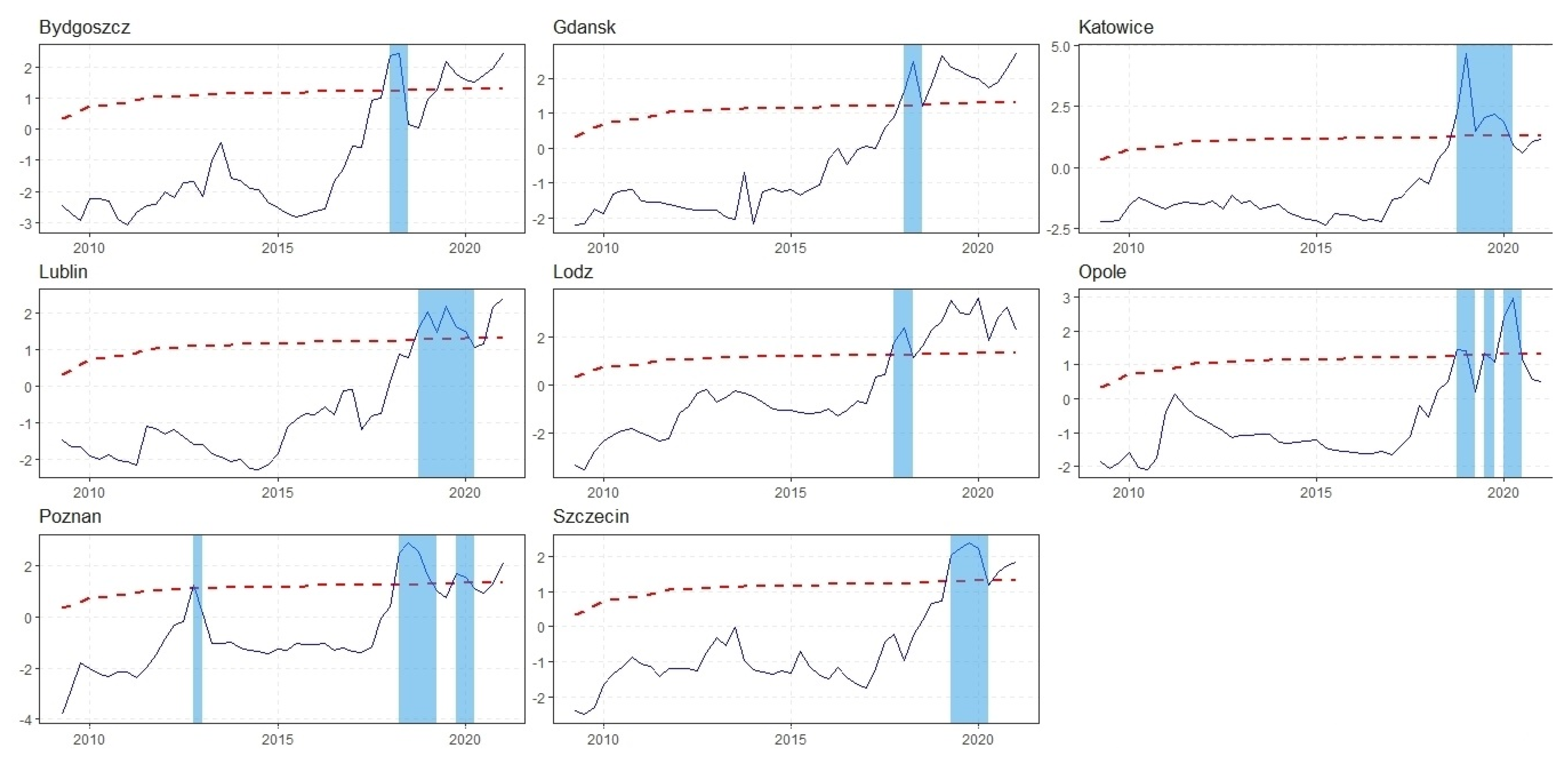
In Figure 5 we see a graphical representation of the episodes of price exuberance for a selection of eight Polish cities.
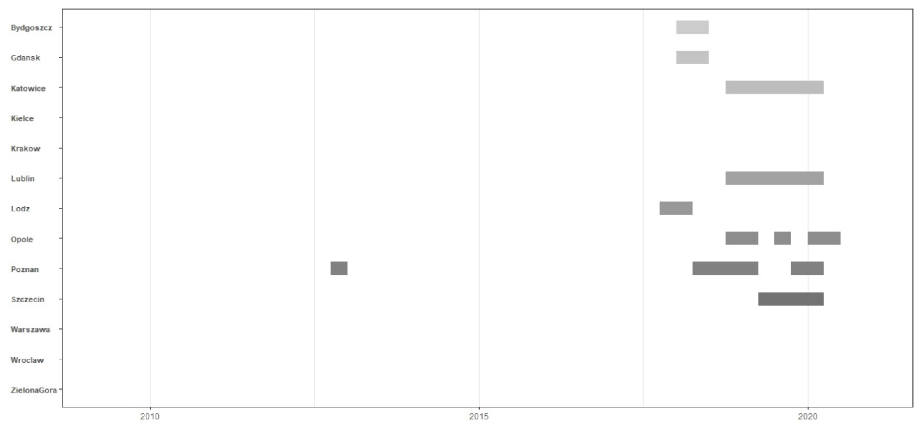
In turn, Figure 6 illustrates the chronology of the identified periods of exuberance in housing prices for a selection of different Polish cities. It shows a cluster of periods of price exuberance from 2017 onwards. Clustering results over our sample period indicate the possibility that some common factor may have contributed to the spread of explosive dynamics in housing prices across different Polish cities.
For panel data of real housing prices, the results indicate that the null hypothesis of a unit root can be rejected at all conventional levels, providing strong evidence of mild explosive dynamics in housing prices time series (see Table 3). In contrast, there is no evidence of exuberance in housing prices for the price-to-income ratio.

5. Discussion

The results provide empirical evidence for the existence of episodes of exuberance in the housing markets of most of the Polish cities under study (13 out of 17), when taking into account the real housing prices. The situation looks differently when the same research method is applied to the price-to-income ratio. In the latter case, mild explosive dynamics in housing prices time series were observed only in two instances, i.e., for Gdynia and Rzeszów. Insofar as other cities are concerned, there is no evidence of any exuberance of housing prices in the period under study. Looking through the prism of purchasing power parity and the increasing creditworthiness of housing purchasers—on the one hand, rising incomes are a catalyst for growth in housing markets, but on the other hand, they mitigate the emergence of price bubbles by correcting them through their internal dynamics.
In the study, we aimed at examining whether there is price exuberance in the housing markets of major Polish cities by testing two different sets of data (time series), i.e., the real rate of change of housing prices and the price-to-income ratio. For this purpose, we applied the SADF and GSADF testing methods used to identify mild explosive dynamics in time series, i.e., methods based on Monte Carlo simulations or bootstrapping. In our study, this simulation consisted of 2000 replications for each observation. The SADF and GSADF test statistics for price-to-income ratio were found to be statistically insignificant in the vast majority of cases (13 out of 17 cases). In other words, following Phillips et al. (2015a), the results of the study provide empirical evidence of speculative bubbles in the case of real housing prices, while no similar episodes of explosiveness (or exuberance) were observed for the price-to-income ratio. Moreover, the SADF and GSADF tests and the date-stamping approach indicate that periods of price exuberance predominantly started to occur only after 2017, i.e., coinciding with the beginning of the dynamic upward trend in these markets (see Figure 1).
The answer to the question of whether there is indeed already a situation of price bubbles in local housing markets in Poland is of course crucial for the participants of this market, but it must also remain important for the monetary authorities implementing monetary and macroprudential policies in Poland. The results show that when analysing changes in housing prices through the lens of rising average incomes, which in many cases have risen faster than housing prices themselves, there is no indication of the emergence of bubbles.
In recent years, there has been an ongoing debate about the formation of housing bubbles (Żelazowski 2018; Korzeb 2019; Czerniak and Kawalec 2020). Housing values have been rising, but this is unlikely to have resulted in a macroeconomic expansion effect. With the increased wealth of Poles due to rising incomes, there has been some price realignment, which should not be surprising given the increase in housing prices worldwide. When assessing the Polish housing markets, one should not forget about the international context, which always creates a certain demand pressure in competitive markets. In this regard, there is evidence of episodic bubbles in many housing markets, including New Zealand (Greenaway-McGrevy and Phillips 2016), Australia (Shi et al. 2016), the United States and the United Kingdom (Kholodilin and Michelsen 2018). In part, this situation results from the artificial creation of money, which, to some degree, also finds its way into the system of housing markets. The blame for this state of affairs should be attributed to the US Federal Reserve, which for the past 12 years has been implementing the monetary policy of “printing money” (Vogiazas and Alexiou 2017). Vogiazas and Alexiou (2017) point to the impact of excessive liquidity and credit financing on the formation of housing bubbles. Indeed, housing bubbles are a product of poor government policies that perpetuate an environment of rising housing prices, making houses unattainable for many young adults (Thornton 2009). Moreover, there are country-specific factors that significantly increase the demand for housing in Poland. The average number of dwellings per 1000 inhabitants (352), currently places Poland in the penultimate place in the EU, and in this respect, Poland is second only to Slovakia (Sobieraj 2020). More importantly, the median age of the population in Poland (40.8) is estimated at a level far below the European average (43.1), which will also, at least for some time, be a source of demand for housing among young people. Of course, the process of rural–urban migration, and the urban transformation that this phenomenon entails, is still ongoing. According to demographic forecasts for Poland until 2030, over the next 10 years metropolises will grow and villages will become even more depopulated. In addition, the Polish government focuses very intensively on infrastructure investments, especially in transportation (construction of a motorway network), but it also supports housing construction in the form of various programmes (Sobieraj 2020). For example, programmes such as: “Family on its own”, and “Flats for newlyweds”, etc. (Sobieraj 2020). This means that the aspect of some government support is also important (Bryx 2017). In addition, there is also speculative demand, which is fuelled by near-zero interest rates and the resulting lack of alternatives for capital investment. Of course, one can hope that the coronavirus pandemic will reverse some of these trends and cause people to move out of city centres, but for the time being it is too early to make any generalisations in this respect.
Finally, comparing this study with Żelazowski’s (2018), it is worth noting that Żelazowski’s study covers the period until 2016, when a significant upward trend in the Polish real estate market was just beginning. More specifically, this study covers the period of the last 59 quarters, the last of which is the first quarter of 2021, so the data already cover the period of a robust upward trend that started in 2016. Importantly, the bubbles we have detected relate mainly to this period. Before that, we were actually dealing with stable prices over a long period of time. The data Żelazowski relies on in his study practically does not cover the last bull market that started (outside Żelazowski’s data window). Unlike him, we present a comparison that clearly shows that in the case of the real prices data (transactional secondary market housing prices) we are dealing with bubbles on a large scale. In contrast, when we look at fundamentals, these bubbles are no longer visible. We also show this in a panel approach, which Żelazowski does not. Our goal is to shed light on this. After all, the debate about whether or not we are dealing with bubbles has been going on in public discourse for years. Moreover, Żelazowski does not call attention to the issue of sensitivity of GSADF tests to window length. We shed light on this issue and present tests for three window lengths, i.e., for 8, 10 and 12 periods. Again, some differences can be seen. For example, the GSADF tests performed for the price-to-income ratio show the existence of an episode of price exuberance in Gdynia, but only for a window length of eight periods. Although, in fact, the window length of 10 periods chosen by Żelazowski seems appropriate.

6. Conclusions

The aim of the study was to examine the occurrence of episodes of exuberance in housing prices across major Polish cities, taking into account quarterly data from Q3 2006 to Q1 2021. In addition to the evolution of real housing prices, we applied the same research method to evaluate time series capturing the changes in prices in relation to average incomes. Disagreeing with the line of reasoning presented by Lind (2009), who believed that bubbles should be defined solely in terms of the price action (i.e., price evolution), we sought to determine whether a fundamental perspective that takes into account purchasing power parity significantly affects the results and changes the context in which these markets are appraised. With regard to real prices from the secondary market, we were able to demonstrate the existence of episodes of price exuberance for 13 of the 17 studied cities. When we changed the context of the study and performed the same tests for the price-to-income ratio, we found that episodes of price exuberance could only be indicated in 2 cases out of the 17. The overall conclusion is that rising average incomes tend to mitigate explosive dynamics, and change the context in which the whole issue of housing bubbles is viewed.
When we look at the results of the SADF and GSADF tests, there are significant differences. As far as the former is concerned, rejections of the null hypothesis have not occurred at all. In contrast, for the GSADF tests, the null hypothesis of a unit root was rejected for 13 out of 17 cities, at different levels of significance, i.e., 1%, 5% or 10%. Thus, we are dealing with evidence for the existence of explosiveness (or exuberance) in real housing prices. In general, the GSADF tests for real housing prices are indicative of the existence of episodes of mild explosive dynamics, while the same statement will not be valid for the price-to-income ratio. In the case of the latter, we were able to provide empirical evidence for the existence of periods of exuberance in real house prices in only two cases, i.e., for Gdynia and Rzeszów.
As for the future direction of the research, it is worthwhile to perform a comparative analysis of several methods presented in Table 1, e.g., LPPL, ARDL bound test, GSADF, bivariate coexplosive VAR, Markov regime switching, Kalman filter and GMM, etc. It is also worth considering the use of disposable income as it determines the real purchasing power of buyers; nominal income may grow and those interested in purchasing a home may have limited unallocated resources with which to pay their obligations, such as those related to mortgage repayments, in a timely manner. It would likely provide better control for housing market fundamentals, and thereby would likely significantly reduce the likelihood of false positive identification.

Author Contributions

Conceptualization, J.S.; methodology, D.M.; validation, J.S. and D.M.; investigation, J.S. and D.M.; resources, D.M.; data curation, D.M.; writing—original draft preparation, J.S. and D.M.; writing—review and editing, J.S. and D.M.; visualization, D.M.; supervision, J.S. All authors have read and agreed to the published version of the manuscript.

Funding

This research received no external funding.

Institutional Review Board Statement

Not applicable.

Informed Consent Statement

Not applicable.

Data Availability Statement

The data presented in this study were from NBP (National Bank of Poland) and the Central Statistical Office (GUS).

Conflicts of Interest

The authors declare no conflict of interest.

Notes

1
The wealth effect is a behavioral economic theory suggesting that people spend more as the value of their assets rise. The idea is that consumers feel more financially secure and confident about their wealth when their homes or investment portfolios increase in value.
2
Irrational exuberance is defined as a rise in asset prices to levels that are not fundamentally justified. It happens as a result of investors’ excessive enthusiasm dictated by their inexplicable market optimism, which has no real basis in fundamental valuation. Such excessive enthusiasm is due to psychological factors.
3
This method is based on recursive ADF regression estimation, employing the Sherman-Morrison-Woodbury formula to efficiently update the least squares estimates as the subsample size changes.
4
It is recommended that the minimum window size should be r 0 = 0.01 + 1.8 / T (Phillips et al. 2015a, 2015b).
5
The remaining variables are defined as in the previous sub-section.
6
The overall assumption is that γ i , r 1 , r 2 may vary from panel to panel as opposed to canonical approaches.

References

  1. Abolafia, Mitchel Y., and Martin Kilduff. 1988. Enacting market crisis: The social construction of a speculative bubble. Administrative Science Quarterly 1: 177–93. [Google Scholar] [CrossRef]
  2. Allen, Franklin, and Elena Carletti. 2013. Systemic risk from real estate and macro-prudential regulation. International Journal of Banking, Accounting and Finance 5: 28–48. [Google Scholar] [CrossRef]
  3. Anderson, Theodore Wilbur, and Cheng Hsiao. 1981. Estimation of Dynamic Models with Error components. Journal of the American Statistical Association 76: 598–606. [Google Scholar] [CrossRef]
  4. Ardila, Diego, Peter Cauwels, Dorsa Sanadgol, and Didier Sornette. 2013. Is There a Real Estate Bubble in Switzerland? arXiv arXiv:1303.4514. [Google Scholar]
  5. Arellano, Manuel, and Stephen Bond. 1991. Some tests of specification for panel data: Monte Carlo evidence and an application to employment equations. The Review of Economic Studies 58: 277–97. [Google Scholar] [CrossRef] [Green Version]
  6. Arellano, Manuel, and Olympia Bover. 1995. Another look at instrumental variable estimation of error component models. Journal of Econometrics 68: 29–51. [Google Scholar] [CrossRef] [Green Version]
  7. Balcerzak, Aadam P. 2009. Wpływ polityki monetarnej Stanów Zjednoczonych na powstanie przyczyn światowego kryzysu gospodarczego z roku 2008. Acta Universitatis Nicolai Copernici Ekonomia 40: 131–46. [Google Scholar]
  8. Basco, Sergi. 2014. Globalization and financial development: A model of the Dot-Com and the Housing Bubbles. Journal of International Economics 92: 78–94. [Google Scholar] [CrossRef]
  9. Blanchard, Olivier, and Mark W. Watson. 1982. Bubbles, Rational Expectations and Financial Markets. In Crises in the Economic and Financial Structure. Edited by Paul Wachter. Lexington: Lexington Books, pp. 295–315. [Google Scholar]
  10. Bond, Stephen. 2002. Dynamic Panel Data Models: A Guide to Micro Data Methods and Practice. Portuguese Economic Journal 1: 141–62. [Google Scholar] [CrossRef]
  11. Bordo, Michael D., and Olivier Jeanne. 2002. Boom-Busts in Asset Prices, Economic Instability, and Monetary Policy (National Bureau of Economic Research Working Paper Series no. w8996). Cambridge: NCBR. [Google Scholar]
  12. Bordo, Michael D., and John Landon-Lane. 2013. Does Expansionary Monetary Policy Cause Asset Price Booms; Some Historical and Empirical Evidence (National Bureau of Economic Research Working Paper Series no. w19585). National Bureau of Economic Research. Cambridge: NCBR. [Google Scholar]
  13. Brunnermeier, Markus, and Christian Julliard. 2008. Money illusion and housing frenzies. The Review of Financial Studies 21: 135–80. [Google Scholar] [CrossRef]
  14. Bryx, Marek. 2017. Market Protection of Flat Buyers as a Part of Housing Policy in Poland. World of Real Estate Journal 102: 75–80. [Google Scholar]
  15. Calem, Paul, and Michael LaCour-Little. 2004. Risk-based capital requirements for mortgage loans. Journal of Banking & Finance 28: 647–72. [Google Scholar]
  16. Caselli, Francesco, Gerardo Esquivel, and Fernando Lefort. 1996. Reopening the Convergence Debate: A New Look At Cross-Country Growth Empirics. Journal of Economic Growth 1: 363–89. [Google Scholar] [CrossRef] [Green Version]
  17. Caspi, Itamar. 2016. Testing for a housing bubble at the national and regional level: The case of Israel. Empirical Economics 51: 483–516. [Google Scholar] [CrossRef] [Green Version]
  18. Ciżkowicz, Piotr, and Adrzej Rzońca. 2010. Stopy procentowe bliskie zera nie muszą być dobrą odpowiedzią na kryzys (BRE Bank—CASE Seminar Proceedings, No. 111). In Banki centralne w zarządzaniu kryzysem finansowym—Strategie wyjścia. Edited by Piotr Ciżkowicz, Andrzej Rzońca and Dobiesła Tymoczko. Warsaw: Center for Social and Economic Research (CASE). [Google Scholar]
  19. Coskun, Yener, and Arvydas Jadevicius. 2017. Is there a housing bubble in Turkey. Real Estate Management and Valuation 25: 48–73. [Google Scholar] [CrossRef] [Green Version]
  20. Coskun, Yener, Ünal Seven, Hasan Murat Ertugrul, and Ali Alp. 2020. Housing price dynamics and bubble risk: The case of Turkey. Housing Studies 35: 50–86. [Google Scholar] [CrossRef]
  21. Czerniak, Adam. 2014. Wpływ cech Społeczno-Kulturowych Społeczeństw na Powstawanie Baniek Cenowych na Rynku Mieszkaniowym. Warsaw: Warsaw School of Economics. [Google Scholar]
  22. Czerniak, Adam, and Stefan Kawalec. 2020. Is a Bubble Inflating on Poland’s Housing Market? mBank-CASE Seminar Proceedings No. 164/2020. Warsaw: CASE—Centrum Analiz Społeczno-Ekonomicznych—Fundacja Naukowa. [Google Scholar]
  23. Czerniak, Adam, and Bartosz Witkowski. 2016. Model Wczesnego Ostrzegania Przed Bańkami Cenowymi na Rynku Mieszkaniowym (Materiały i Studia Narodowego Banku Polskiego Numer 326.). Warsaw: NBP (Narodowy Bank Polski). [Google Scholar]
  24. De Bandt, Olivier, Thomas Knetsch, Juan Peñalosa, and Francesco Zollino. 2010. Housing Markets in Europe: A Macroeconomic Perspective. Berlin: Springer. [Google Scholar]
  25. Diba, Behzad T., and Herschel I. Grossman. 1984. Rational Bubbles in the Price of Gold (No. w1300). Cambridge: National Bureau of Economic Research. [Google Scholar]
  26. Diba, Behzad T., and Herschel I. Grossman. 1988. Explosive rational bubbles in stock prices? The American Economic Review 78: 520–30. [Google Scholar]
  27. Dreger, Christian, and Konstantin A. Kholodilin. 2013. An early warning system to predict speculative house price bubbles. Economics 7: 20130008. [Google Scholar] [CrossRef] [Green Version]
  28. Elliott, Douglas J., and Martin Neil Baily. 2009. Telling the Narrative of the Financial Crisis: Not Just a Housing Bubble. Washington, DC: Brookings Institution. [Google Scholar]
  29. Engsted, Tom, and Bent Nielsen. 2012. Testing for rational bubbles in a coexplosive vector autoregression. The Econometrics Journal 15: 226–54. [Google Scholar] [CrossRef] [Green Version]
  30. Engsted, Tom, Simon Juul Hviid, and Thomas Quistgaard Pedersen. 2016. Explosive bubbles in house prices? Evidence from the OECD countries. Journal of International Financial Markets, Institutions and Money 40: 14–25. [Google Scholar] [CrossRef]
  31. Escobari, Diego, Damian S. Damianov, and Andres Bello. 2015. A time series test to identify housing bubbles. Journal of Economics and Finance 39: 136–52. [Google Scholar] [CrossRef] [Green Version]
  32. European Central Bank. 2010. Asset Price Bubbles and Monetary Policy Revisited (Monthly Bulletin, November). Frankfurt am Main: European Central Bank. [Google Scholar]
  33. Eurostat. 2021. House Prices—Quarterly and Annual Rates of Change, 2019Q4-2020Q3 (%). Available online: https://ec.europa.eu/eurostat/statistics-explained/index.php?title=File:House_Prices_%E2%80%93_Quarterly_and_annual_rates_of_change,_2019Q4-2020Q3_(%25).png (accessed on 24 August 2021).
  34. Evans, George W. 1991. Pitfalls in testing for explosive bubbles in asset prices. The American Economic Review 81: 922–30. [Google Scholar]
  35. Flotyński, Marcin. 2020. Działania Narodowego Banku Polskiego na rzecz utrzymania stabilności ekonomicznej w czasie kryzysu wywołanego pandemią koronawirusa w świetle uwarunkowań makroekonomicznych. In Przedsiębiorstwo, Gospodarka i Społeczeństwo w Kręgu Zainteresowania Ekonomistów. Edited by Ryszard Kamiński. Poznań: Wydawnictwo Polskiego Towarzystwa Ekonomicznego Oddział w Poznaniu. [Google Scholar]
  36. Greenaway-McGrevy, Ryan, and Peter C. B. Phillips. 2016. Hot property in New Zealand: Empirical evidence of housing bubbles in the metropolitan centres. New Zealand Economic Papers 50: 88–113. [Google Scholar] [CrossRef]
  37. Gürkaynak, Refet S. 2008. Econometric tests of asset price bubbles: Taking stock. Journal of Economic Surveys 22: 166–86. [Google Scholar] [CrossRef]
  38. Hall, Stephen G., Zacharias Psaradakis, and Martin Sola. 1999. Detecting periodically collapsing bubbles: A Markov-switching unit root test. Journal of Applied Econometrics 14: 143–54. [Google Scholar] [CrossRef]
  39. Hamilton, James D., and Charles H. Whiteman. 1985. The observable implications of self-fulfilling expectations. Journal of Monetary Economics 16: 353–73. [Google Scholar] [CrossRef]
  40. Holtz-Eakin, Douglas, Whitney Newey, and Harvey S. Rosen. 1988. Estimating vector Autoregressions with panel data. Econometrica: Journal of the Econometric Society 56: 1371–95. [Google Scholar] [CrossRef]
  41. Homm, Ulrich, and Jörg Breitung. 2012. Testing for speculative bubbles in stock markets: A comparison of alternative methods. Journal of Financial Econometrics 10: 198–231. [Google Scholar] [CrossRef]
  42. Iacoviello, Matteo. 2010. Housing in DSGE models: Findings and new directions. In Housing Markets in Europe. Berlin/Heidelberg: Springer. [Google Scholar]
  43. Iacoviello, Matteo, and Stefano Neri. 2010. Housing market spillovers: Evidence from an estimated DSGE model. American Economic Journal: Macroeconomics 2: 125–64. [Google Scholar] [CrossRef] [Green Version]
  44. Im, Kyung So, Mohammad Hashem Pesaran, and Yongcheol Shin. 2003. Testing for unit roots in heterogeneous panels. Journal of Econometrics 115: 53–74. [Google Scholar] [CrossRef]
  45. Jadevicius, Arvydas, and Simon Huston. 2015. ARIMA modelling of Lithuanian house price index. International Journal of Housing Markets and Analysis 8: 135–47. [Google Scholar] [CrossRef]
  46. Kamiński, Maciej. 2019. The Theoretical Model of Polish Housing Policy between 2002 and 2016. Folia Oeconomica Stetinensia 19: 20–30. [Google Scholar] [CrossRef] [Green Version]
  47. Kholodilin, Konstantin, and Claus Michelsen. 2018. Signs of new housing bubble in many OECD countries: Lower risk in Germany. DIW Weekly Report 8: 275–85. [Google Scholar]
  48. Kim, Kyung-Hwan. 2004. Housing and the Korean economy. Journal of Housing Economics 13: 321–41. [Google Scholar] [CrossRef]
  49. Kivedal, Bjørnar Karlsen. 2013. Testing for rational bubbles in the US housing market. Journal of Macroeconomics 38: 369–81. [Google Scholar] [CrossRef]
  50. Korzeb, Zbigniew. 2019. The Real Estate and Credit Bubble in Spain. Implications for Poland. Problems of World Agriculture 19: 77–88. [Google Scholar] [CrossRef] [Green Version]
  51. Leijten, Ingrid, and Kaisa de Bel. 2020. Facing financialization in the housing sector: A human right to adequate housing for all. Netherlands Quarterly of Human Rights 38: 94–114. [Google Scholar] [CrossRef]
  52. LeRoy, Stephen F., and Richard D. Porter. 1981. The Present-Value Relation: Tests Based on Implied Variance Bonds. Econometrica 49: 555–74. [Google Scholar] [CrossRef]
  53. Lin, Li, Ruoen Ren, and Didier Sornette. 2009. A Consistent Model of’Explosive’Financial Bubbles with Mean-Reversing Residuals. Swiss Finance Institute Research Paper, (09–14). Zürich: Swiss Finance Institute. [Google Scholar]
  54. Lind, Hans. 2009. Price bubbles in housing markets: Concept, theory and indicators. International Journal of Housing Markets and Analysis. International Journal of Housing Markets and Analysis 2: 78–90. [Google Scholar] [CrossRef]
  55. Machaj, Mateusz. 2016. Can the Taylor Rule be a good guidance for policy? The case of 2001–2008 real estate bubble. Prague Economic Papers 25: 381–95. [Google Scholar] [CrossRef]
  56. Maddala, Gangadharrao Soundalyarao, and Shaowen Wu. 1999. A comparative study of unit root tests with panel data and a new simple test. Oxford Bulletin of Economics and Statistics 61: 631–52. [Google Scholar] [CrossRef]
  57. Malkiel, Burton G. 2010. Bubbles in Asset Prices (CEPS Working Paper No. 200). Brussels: Centre for European Policy Studies. [Google Scholar]
  58. Martinez-Garcia, Enrique, Efthymios (Themis) Pavlidis, and Kostas Vasilopoulos. 2020. Exuber: Recursive Right-Tailed Unit Root Testing with R (No. w383). Dallas: Globalization and Monetary Policy Institute. [Google Scholar]
  59. Martori, Joan Carles, Rafa Madariaga, and Ramon Oller. 2016. Real estate bubble and urban population density: Six Spanish metropolitan areas 2001–2011. The Annals of Regional Science 56: 369–92. [Google Scholar] [CrossRef]
  60. NBP. 2019. Information on Housing Prices and the Situation on the Residential Real Estate Market in Poland in the Second Quarter of 2019. Warsaw: Narodowy Bank Polski (NBP). [Google Scholar]
  61. NBP. 2021. Cykliczne Materiały Analityczne NBP. Available online: https://www.nbp.pl/home.aspx?f=/publikacje/rynek_nieruchomosci/index2.html (accessed on 21 August 2021).
  62. Ng, Eric C. 2015. Housing market dynamics in China: Findings from an estimated DSGE model. Journal of Housing Economics 29: 26–40. [Google Scholar] [CrossRef]
  63. Oust, Are, and Kjartan Hrafnkelsson. 2017. What is a housing bubble? Economics Bulletin 37: 806–36. [Google Scholar]
  64. Paries, Matthieu Darracq, and Alessandro Notarpietro. 2008. Monetary Policy and Housing Prices in an Estimated DSGE Model for the US and the Euro Area. Frankfurt: European Central Bank. [Google Scholar]
  65. Pavlidis, Efthymios, Alisa Yusupova, Ivan Paya, David Peel, Enrique Martínez-García, Adrienne Mack, and Valerie Grossman. 2016. Episodes of exuberance in housing markets: In search of the smoking gun. The Journal of Real Estate Finance and Economics 53: 419–49. [Google Scholar] [CrossRef] [Green Version]
  66. Pedersen, Thomas Quistgaard, and Erik Christian Montes Schütte. 2020. Testing for explosive bubbles in the presence of autocorrelated innovations. Journal of Empirical Finance 58: 207–25. [Google Scholar] [CrossRef]
  67. Pesaran, Mohammad Hashem, and Yongcheol Shin. 1999. An autoregressive distributed lag modelling approach to cointegration analysis. In Econometrics and Economic Theory in the 20th Century: The Ragnar Frisch Centennial Symposium. Edited by Steinar Strom. Cambridge: Cambridge University Press. [Google Scholar]
  68. Pesaran, Mohammad Hashem, Yongcheol Shin, and Richard J. Smith. 2001. Bounds testing approaches to the analysis of level relationships. Journal of Applied Econometrics 16: 289–326. [Google Scholar] [CrossRef]
  69. Phillips, Peter C. B., Yangru Wu, and Jun Yu. 2011. Explosive behavior in the 1990s Nasdaq: When did exuberance escalate asset values? International Economic Review 52: 201–26. [Google Scholar] [CrossRef] [Green Version]
  70. Phillips, Peter C. B., Shuping Shi, and Jun Yu. 2014. Specification sensitivity in right-tailed unit root testing for explosive behaviour. Oxford Bulletin of Economics and Statistics 76: 315–33. [Google Scholar] [CrossRef]
  71. Phillips, Peter C. B., Shuping Shi, and Jun Yu. 2015a. Testing for multiple bubbles: Historical episodes of exuberance and collapse in the S&P 500. International Economic Review 56: 1043–78. [Google Scholar]
  72. Phillips, Peter C. B., Shuping Shi, and Jun Yu. 2015b. Testing for multiple bubbles: Limit theory of real-time detectors. International Economic Review 56: 1079–134. [Google Scholar] [CrossRef] [Green Version]
  73. Quigley, John M. 2002. Real estate prices and economic cycles. International Real Estate Review 2: 1–20. [Google Scholar]
  74. Rubio, Margarita, and José A. Carrasco-Gallego. 2016. Liquidity, interest rates and house prices in the euro area: A DSGE analysis. Journal of European Real Estate Research 9: 4–25. [Google Scholar] [CrossRef] [Green Version]
  75. Said, Rosli, Alaistair Adair, Stanley McGreal, and Rohayu Majid. 2014. Inter-relationship between the housing market and housing finance system: Evidence from Malaysia. International Journal of Strategic Property Management 18: 138–50. [Google Scholar] [CrossRef] [Green Version]
  76. Samirana, Sanja. 2020. Testing for bubbles in the Indian housing market: And ARDL bounds testing approach. Journal of International Money, Banking and Finance 1: 87–107. [Google Scholar]
  77. Shi, Shuping. 2013. Specification sensitivities in the Markov-switching unit root test for bubbles. Empirical Economics 45: 697–713. [Google Scholar] [CrossRef]
  78. Shi, Shuping. 2017. Speculative bubbles or market fundamentals? An investigation of US regional housing markets. Economic Modelling 66: 101–11. [Google Scholar] [CrossRef] [Green Version]
  79. Shi, Shuping, and Yong Song. 2015. Identifying speculative bubbles using an infinite hidden Markov model. Journal of Financial Econometrics 14: 159–84. [Google Scholar] [CrossRef] [Green Version]
  80. Shi, Shuping, Abbas Valadkhani, Russell Smyth, and Farshid Vahid. 2016. Dating the timeline of house price bubbles in Australian capital cities. Economic Record 92: 590–605. [Google Scholar] [CrossRef]
  81. Shiller, Robert J. 1981. Do Stock Prices Move Too Much to be Justified by Subsequent Changes in Dividends? American Economic Review 71: 421–36. [Google Scholar]
  82. Shiller, Robert J. 2003. From efficient markets theory to behavioral finance. Journal of Economic Perspectives 17: 83–104. [Google Scholar] [CrossRef] [Green Version]
  83. Siwiński, Włodzimierz. 2011. Globalny kryzys gospodarczy i jego implikacje dla polityki pieniężnej. Master of Business Administration 19: 10–29. [Google Scholar]
  84. Slavata, David. 2018. The Comparison of Housing Affordability of Czech and Polish Regions. In Development and Administration of Border Areas of the Czech Republic and Poland, Support for Sustainable Development, Proceedings of the 2nd International Scientific Conference (VŠB-TU Ostrava), Ostrava, Czech Republic, 11–12 September 2018. Ostrava: VŠB-TU Ostrava. [Google Scholar]
  85. Sobieraj, Janusz. 2020. Investment Project Management on the Housing Construction Market. Madrid: Aurum Universitas Grupo Hespérides. [Google Scholar]
  86. Sobieraj, Janusz, and Dominik Metelski. 2021. Application of the Bayesian New Keynesian DSGE Model to Polish Macroeconomic Data. Engineering Economics 32: 140–53. [Google Scholar] [CrossRef]
  87. Solak, Ali Osman, and Burhan Kabaday. 2016. Bounds Testing Approaches to Housing Demand in Turkey: Is There a Real Estate Bubble? International Journal of Economics and Financial Issues 6: 1132–35. [Google Scholar]
  88. Sornette, Didier. 2004. Why stock markets crash: Critical events in complex financial systems. Physics Today 57: 78–79. [Google Scholar]
  89. Thornton, Mark. 2009. The economics of housing bubbles. In Housing America: Building out of a Crisis. Edited by Randall G. Holcombe and Benjamin Powell. New Brunswick: Transaction Publishers. [Google Scholar]
  90. Tirole, Jean. 1985. Asset Bubbles and Overlapping Generations. Econometrica 53: 1499–528. [Google Scholar] [CrossRef]
  91. Tirtiroǧlu, Doǧan. 1992. Efficiency in housing markets: Temporal and spatial dimensions. Journal of Housing Economics 2: 276–92. [Google Scholar] [CrossRef]
  92. Trojanek, Radosław. 2008. Wahania cen na rynku mieszkaniowym. Poznań: Wydawnictwo Akademii Ekonomicznej w Poznaniu. [Google Scholar]
  93. Visco, Ignazio. 2005. Comments on Recent Experiences with Asset Prices Bubbles. In Asset Price Bubbles: The Implications for Monetary Policy, Regulatory, and International Policies. Edited by William Curt Hunter, George G. Kaufman and Michael Pomerleano. Cambridge: The MIT Press, pp. 165–71. [Google Scholar]
  94. Vogiazas, Sofoklis, and Constantinos Alexiou. 2017. Determinants of housing prices and bubble detection: Evidence from seven advanced economies. Atlantic Economic Journal 45: 119–31. [Google Scholar] [CrossRef] [Green Version]
  95. Wang, Pengfei, and Yi Wen. 2012. Speculative bubbles and financial crises. American Economic Journal: Macroeconomics 4: 184–221. [Google Scholar] [CrossRef]
  96. Wang, Lipo, Fung Foong Chan, Yaoli Wang, and Qing Chang. 2016. Predicting public housing prices using delayed neural networks. Paper presented at the 2016 IEEE TENCON Region 10 Conference, Singapore, November 22–26. [Google Scholar]
  97. Wei, Yigang, Yan Li, Jing Li, Yang Wang, and Zeyu Qiang. 2020. Regional and longitudinal disparity of housing bubbles in US markets: Evidence from GSADF tests. Journal of Urban Planning and Development 146: 1–14. [Google Scholar] [CrossRef]
  98. Widłąk, Marta. 2010. Dostosowanie Indeksów Cenowych do Zmian Jakości. Metoda Wyznaczania Hedonicznych Indeksów Cen i Możliwości Ich Zastosowania dla Rynku Mieszkaniowego (Materiały i Studia NBP, 247). Warsaw: Narodowy Bank Polski (Departament Edukacji i Wydawnictw). [Google Scholar]
  99. Wijburg, Gertjan. 2020. The de-financialization of housing: Towards a research agenda. Housing Studies, 1–18. [Google Scholar] [CrossRef]
  100. Winiecki, Jan. 2013. Świat darmowego pieniądza i jego dotychczasowe konsekwencje. BRE Bank-CASE Papers 129: 21–25. [Google Scholar]
  101. Woźniak, Przemysław, and Jan Winiecki. 2013. Długofalowe Skutki Polityki Niskich Stóp i Poluzowania Polityki Pieniężnej. Warsaw: Center for Social and Economic Research (CASE). [Google Scholar]
  102. Xiao, Qin, and Steven Devaney. 2016. Are mortgage lenders guilty of the housing bubble? A UK perspective. Applied Economics 48: 4271–90. [Google Scholar] [CrossRef]
  103. Żelazowski, Konrad. 2018. Identyfikacja baniek cenowych na lokalnych rynkach mieszkaniowych w Polsce z wykorzystaniem testu GSADF. Świat Nieruchomości 2: 5–10. [Google Scholar]
  104. Zeren, Feyyaz, and Oylum Şehvez Ergüzel. 2015. Testing for bubbles in the housıng market: Further evidence from Turkey. Financial Studies 19: 40–52. [Google Scholar]
  105. Zhang, Lu, and Dirk Bezemer. 2014. How the Credit Cycle Affects Growth: The Role of Bank Balance Sheets (SOM Research Reports; Vol. 14026-GEM). Groningen: University of Groningen, SOM Research School. [Google Scholar]
  106. Zhao, Xiaobin, Hongyu Zhan, Yanpeng Jiang, and Wenjun Pan. 2017. How big is China’s real estate bubble and why hasn’t it burst yet? Land Use Policy 64: 153–62. [Google Scholar] [CrossRef]
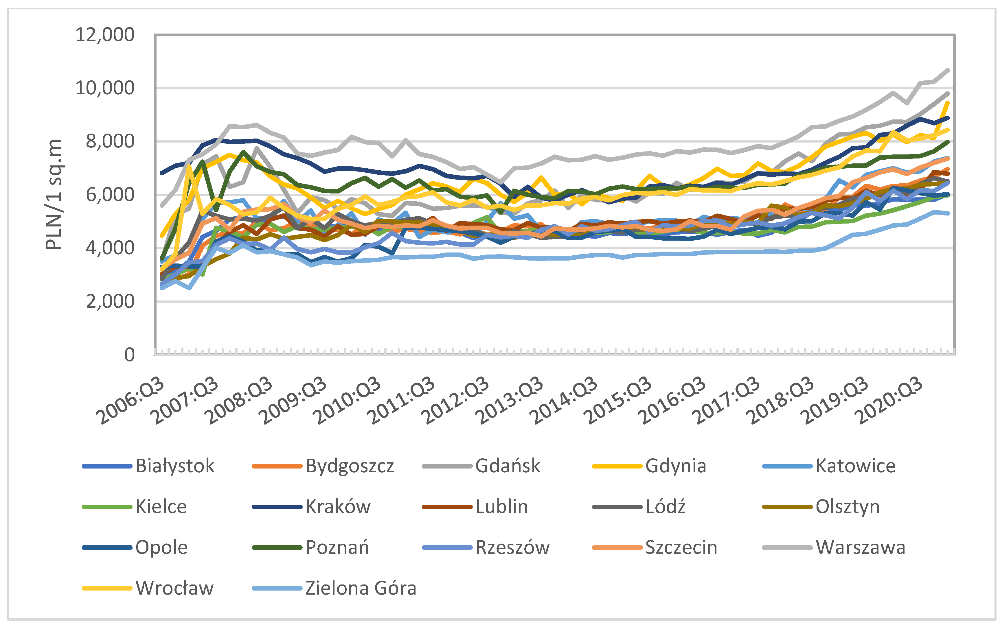
Figure 1. Transaction prices on secondary market—17 Polish cities.
Jrfm 14 00412 g001
Figure 2. Hedonic price index (q-o-q). Secondary market—16 cities.
Jrfm 14 00412 g002
Figure 3. Price-to-income ratio—17 Polish cities.
Jrfm 14 00412 g003
Figure 4. Price-to-income ratio around the World (2020:Q4 or latest available index, 2015 = 100). Source: Organisation for Economic Co-operation and Development.
Jrfm 14 00412 g004
Figure 5. Graphical representation of episodes of price exuberance for a sample of eight Polish cities.
Jrfm 14 00412 g005
Figure 6. Date-stamping periods of exuberance in local housing markets.
Jrfm 14 00412 g006
Table 1. Different research methods in the literature for identifying price bubbles.
MethodCharacteristic of the Scientific MethodApplied by Authors
log-periodic power law (LPPL)LPPL is the fundamental equation that describes the temporal growth of prices before a crash and it has been proposed in different forms in various papers, see e.g., Sornette (2004) and Lin et al. (2009) and references therein.Sornette (2004); Lin et al. (2009); Ardila et al. (2013)
variance bound tests, e.g., Autoregressive Distributed Lag (ARDL) bound testViolation of variance bounds could be attributed to the presence of bubbles. ARDL models have come to play an important role in the modelling of non-stationary time-series data. In particular, they are used to implement the so-called “Bounds Tests” (Pesaran and Shin 1999; Pesaran et al. 2001), to see if long-run relationships are present when we have a group of time-series, some of which may be stationary, while others are not.Shiller (1981); LeRoy and Porter (1981); Blanchard and Watson (1982); Tirole (1985); Pesaran and Shin (1999); Pesaran et al. (2001); Solak and Kabaday (2016); Samirana (2020)
fixed effects ordinary least squares (OLS) regression modelOLS regression is a type of linear least squares method for estimating the unknown parameters in a linear regression model. For example, Basco (2014) conducted a linear regression of house prices on the housing supply elasticity for different sub-periods.Basco (2014)
right-tailed unit root tests (ADF, SADF, GSADF)In statistics, a unit root test tests whether a time series variable is non-stationary and possesses a unit root. The null hypothesis is generally defined as the presence of a unit root and the alternative hypothesis is either stationarity, trend stationarity or explosive root depending on the test used. Right-tailed unit root tests have proved promising for detecting exuberance in economic and financial activities (Phillips et al. 2011, 2014, 2015a, 2015b). Similar to left-tailed tests, the limit theory and test performance are sensitive to the null hypothesis and the model specification used in parameter estimation.Phillips et al. (2014); Zeren and Ergüzel (2015); Caspi (2016); Coskun and Jadevicius (2017);
bivariate coexplosive vector autoregressionThe coexplosive model arises as a restriction to the vector autoregressive model. It allows for common random walk trend and a common explosive stochastic component with explosive root ρ .Engsted and Nielsen (2012); Kivedal (2013); Engsted et al. (2016)
esploratory spatial data analysis ESDAESDA is a set of tools and techniques that allow you to gain insight into your data and construct better interpolation models. Exploratory spatial data analysis (ESDA) is the extension of exploratory data analysis (EDA) to the problem of detecting spatial properties of data sets where, for each attribute value, there is a locational datum. This locational datum references the point or the area to which the attribute refers.Martori et al. (2016)
Markov Regime Switching modelMarkov-switching is introduced to capture asymmetric market behaviours and turning points.Hall et al. (1999); Shi (2013); Shi and Song (2015); Xiao and Devaney (2016)
Ordinary Least Square (OLS), Fully Modified OLS (FMOLS), Dynamic OLS (DOLS)Ordinary Least Square (OLS), Fully Modified OLS (FMOLS), Dynamic OLS (DOLS) can be used to investigate the long-term static and dynamic coefficients between house prices and its determinants. Coskun et al. (2020)
ARIMA modelARIMA models and the selection of forecast performances, can be used, for example, to compare actual and fundamental house prices to determine the existence of a bubble formation. Jadevicius and Huston (2015) applied the ARIMA technique to assess Lithuanian house prices and forecasted 8 per cent house price inflation in the coming year.Jadevicius and Huston (2015); Coskun et al. (2020)
Kalman FilterThe Kalman filter is an efficient recursive filter that estimates the internal state of a linear dynamic system from a series of noisy measurements. It is a “state observer” that minimises the mean square estimation error, meaning that the algorithm estimates the internal state of the object based on measurements of its input and output, and the state estimate is statistically optimal. Originally the Kalman filter is designed to work with linear systems, but with minor modifications it is also possible to work with non-stationary (whose model changes in time) and nonlinear systems.Kim (2004); Coskun et al. (2020)
VAR modelVector autoregression allows modelling the relationship between multiple variables that change over time. This method is used for multivariate forecasting to show how two or more time series affect each other. A VAR can also be considered as a model of a stochastic process. The advantage of this method is that it can take into account information from outside the housing market and account for aggregate economic conditions (Shi 2017).Shi (2017)
generalised method of moments (GMM)Generalised method of moments (GMM) is a good method especially when dealing with a dynamic dimension of a model. GMM was first introduced by Holtz-Eakin et al. (1988) and further developed by Arellano and Bond (1991) and Arellano and Bover (1995). The GMM methodological framework is known to be very effective when dealing with estimation issues such as: bi-directional causality between variables; the possible endogeneity of explanatory variables, as well as omitted variable biases; time invariant country characteristics (fixed effects), that may be correlated with the explanatory variables; and the presence of autocorrelation (Anderson and Hsiao 1981; Caselli et al. 1996; Bond 2002). In addition to the two-step system GMM, we also generate estimates using the standard ordinary least squares (OLS) and fixed effects (or within) specifications.Holtz-Eakin et al. (1988); Arellano and Bond (1991); Arellano and Bover (1995); Vogiazas and Alexiou (2017)
Deviation from the moving average by a certain parameterBordo and Jeanne (2002) proposed a method to detect periods of price exuberance when the three-year moving average of real annual price dynamics exceeds the standard deviation of this moving average multiplied by a parameter of 1.3 for the entire time series. Czerniak (2014), in turn, extended the method of Bordo and Jeanne (2002) by optimising the critical value for the housing market beyond which a price bubble occurs; this value is 1.5% for the 12-quarter moving average of real price dynamics on a quarterly basis. In addition, Bordo and Landon-Lane (2013) developed an indicator that signals the presence of a price bubble when real annualised price growth exceeds 5% for two consecutive years.Bordo and Jeanne (2002); Czerniak (2014); Bordo and Landon-Lane (2013)
Hodrick-Prescott filterThe method based on the Hodrick-Prescott filter can be used to measure whether the deviation of current real housing prices from the trend exceeds a certain critical value. The Hodrick-Prescott filter is one of the most popular mathematical tools in macroeconomics (Sobieraj and Metelski 2021). It can be used to smooth a time series and remove cyclical fluctuations and one-time disturbances from it. For example, Dreger and Kholodilin (2013) developed a method to compute the trend for the logarithm of the real price level using the Hodrick-Prescott filter with a lambda parameter equal to the standard value for a quarterly series (1600), followed by the cyclical component. According to the method of Dreger and Kholodilin (2013), those periods in which the current value of the cyclical component exceeds the standard deviation of the entire time series of this component are called periods of price exuberance. A modification of this method was worked out by Czerniak (2014), who adopted a higher lambda parameter for the Hodrick-Prescott filter, i.e., at the level of 10 to the power of 5.Dreger and Kholodilin (2013); Czerniak (2014); Czerniak and Kawalec (2020)
artificial neural network (ANN)For static ANNs, the neural network model is able to map the non-linear relationship between resale price and those housing characteristics that influence the housing price.Wang et al. (2016)
Table 2. Results for the Univariate ADF, SADF and GSADF Tests.
City/Region Real Housing PricesPrice-to-Income Ratio
ADFSADFGSADFADFSADFGSADF
Panel A: Test Statistics (lag length k = 1 , minimum window size r 0 —8, 10, 12, respectively)
Białystok r 0 = 8 −2.60−2.551.75−1.58−1.010.637
r 0 = 10 −2.60−2.601.75−1.58−1.010.637
r 0 = 12 −2.60−2.601.75−1.58−1.010.637
Bydgoszcz r 0 = 8 −1.56−1.562.46 **−1.77−1.320.548
r 0 = 10 −1.56−1.562.46 **−1.77−1.320.0622
r 0 = 12 −1.56−1.562.46 **−1.77−1.320.0622
Gdańsk r 0 = 8 −0.297 *−0.2972.88 **−1.51−0.8040.926
r 0 = 10 −0.297−0.2972.74 **−1.51−0.8040.828
r 0 = 12 −0.297−0.2972.74 ***−1.51−0.8040.812
Gdynia r 0 = 8 −0.580−0.5800.862−1.44−0.4293.81 ***
r 0 = 10 −0.580−0.5800.862−1.44−0.4290.892
r 0 = 12 −0.580−0.5800.862−1.44−0.4290.892
Katowice r 0 = 8 −1.14−1.144.67 ***−2.42−1.700.437
r 0 = 10 −1.14−1.144.67 ***−2.42−1.700.437
r 0 = 12 −1.14−1.143.64 ***−2.42−1.700.437
Kielce r 0 = 8 −2.82−1.263.87 ***−1.07−0.6241.44
r 0 = 10 −2.82−1.603.87 ***−1.07−0.6241.08
r 0 = 12 −2.82−1.913.87 ***−1.07−0.6240.517
Kraków r 0 = 8 −0.0327 *−0.03272.91 **−2.150.07490.611
r 0 = 10 −0.0327−0.03272.91 **−2.150.07490.447
r 0 = 12 −0.0327−0.03272.91 ***−2.15−0.4720.447
Lublin r 0 = 8 −1.11−0.4782.41 *−1.74−1.270.775
r 0 = 10 −1.11−1.112.41 **−1.74−1.27−0.259
r 0 = 12 −1.11−1.112.41 **−1.74−1.27−0.259
Łódź r 0 = 8 −1.66−1.513.61 ***−1.96−1.54−0.0511
r 0 = 10 −1.66−1.513.61 ***−1.96−1.54−0.0511
r 0 = 12 −1.66−1.513.61 ***−1.96−1.54−0.0511
Olsztyn r 0 = 8 −1.62−1.151.38−1.40−0.7450.0971
r 0 = 10 −1.62−1.551.38−1.40−0.745−0.00214
r 0 = 12 −1.62−1.551.38−1.40−0.745−0.00214
Opole r 0 = 8 −0.949−0.5642.98 **−1.85−1.20−0.0125
r 0 = 10 −0.949−0.5642.98 ***−1.85−1.20−0.136
r 0 = 12 −0.949−0.5642.98 ***−1.85−1.20−0.170
Poznań r 0 = 8 −3.52−3.312.89 **−1.31−0.9500.976
r 0 = 10 −3.52−3.522.89 **−1.31−0.9500.976
r 0 = 12 −3.52−3.522.89 ***−1.31−0.9500.976
Rzeszów r 0 = 8 −1.01−1.011.01−2.07−1.683.21 **
r 0 = 10 −1.01−1.011.01−2.07−1.683.21 **
r 0 = 12 −1.01−1.011.01−2.07−1.683.21 ***
Szczecin r 0 = 8 −0.614−0.6142.38 *−1.39−0.6350.0582
r 0 = 10 −0.614−0.6142.38 **−1.39−0.635−0.266
r 0 = 12 −0.614−0.6142.38 **−1.39−0.635−0.266
Warszawa r 0 = 8 −0.347 *−0.3474.31 ***−1.73−0.4620.507
r 0 = 10 −0.347 *−0.3474.31 ***−1.73−0.4620.507
r 0 = 12 −0.347 *−0.3474.31 ***−1.73−0.4620.507
Wrocław r 0 = 8 −1.99−1.994.68 ***−1.60−0.8251.45
r 0 = 10 −1.99−1.994.68 ***−1.60−0.8251.45
r 0 = 12 −1.99−1.994.68 ***−1.60−0.8251.45
Zielona Góra r 0 = 8 −0.760−0.5924.89 ***−1.79−1.080.725
r 0 = 10 −0.760−0.5924.10 ***−1.79−1.080.260
r 0 = 12 −0.760−0.5924.08 ***−1.79−1.080.260
Panel B: Critical Values
90% r 0 = 8 −0.4081.052.04−0.4271.082.04
r 0 = 10 −0.4081.021.85−0.5050.9971.81
r 0 = 12 −0.3710.8141.55−0.4890.9381.63
95% r 0 = 8 −0.03251.352.42−0.09461.382.39
r 0 = 10 −0.03251.322.13−0.1471.262.06
r 0 = 12 −0.03831.091.89−0.1021.271.98
99% r 0 = 8 0.7352.153.610.3591.913.19
r 0 = 10 0.7352.132.960.5371.903.05
r 0 = 12 0.6511.672.650.6331.802.51
Note: *, ** and *** denote statistical significance at the 10, 5 and 1 percent significance level, respectively. All results are for autoregressive lag length k = 1.
Table 3. Results of the univariate estimation of panel test statistics (GSADF PANEL).
GSADF Panel Test Statistic
Real Housing Prices2.18
Price-to-Income Ratio−0.56
Critical Value
1%5%10%
GSADF PANEL0.3470.2340.218
Publisher’s Note: MDPI stays neutral with regard to jurisdictional claims in published maps and institutional affiliations.