1. Introduction
Volatility is an unobservable variable, unlike returns.
Andersen and Bollerslev (
1998) propose using realized volatility (RV) as a proxy variable for true volatility. This is because there is a theoretical background that RV converges in probability to true volatility when the logarithmic price of assets is a semi-martingale (
Barndorff-Nielsen and Shephard 2002). RV is calculated as the sum of the squares of returns observed frequently during the day. For RV forecasting, various time series models have been suggested per the heterogeneous market hypothesis proposed by
Müller et al. (
1997) and the discovery of the RV’s long-term memory characteristics by
Andersen et al. (
2003), such as the fractionally integrated autoregressive moving average (ARFIMA) model proposed by
Andersen et al. (
2001) and the heterogeneous autoregressive (HAR) model proposed by
Corsi (
2009). The ARFIMA model is well known as a long-term memory process model. In contrast, the HAR model is not a long-term memory process model but well approximates the long-term memory process with a few explanatory variables, which are past daily, weekly and monthly RV, in a linear modeling framework.
Baillie et al. (
2019) report that RV series are quite complex and can involve both HAR components and long memory components.
Watanabe (
2020) remarks that the HAR model is the most commonly used model in recent years for RV time-series modeling as the HAR model can predict RV with high prediction accuracy because of few explanatory variables.
Qiu et al. (
2019) remarked that the HAR model has computational simplicity (e.g., ordinary least squares method) and excellent out-of-sample performance compared to ARFIMA. Various previous studies have followed
Corsi (
2009), expanding and generalizing the HAR model in many directions (
Andersen et al. 2007;
Ubukata and Watanabe 2014;
Bekaert and Hoerova 2014;
Bollerslev et al. 2016;
Luong and Dokuchaev 2018;
Qiu et al. 2019;
Motegi et al. 2020;
Watanabe 2020). In particular,
Luong and Dokuchaev (
2018) introduced a nonlinear model using the random forest method, which is a well-known machine learning method introduced by
Breiman (
2001). They apply the random forest method for forecasting the direction (“up” or “down”) of RV in a binary classification problem framework using a technical indicator of RV.
Linton and Mahmoodzadeh (
2018) report that high-frequency trading (HFT) is the predominant feature in current financial markets due to technological advances and market structure development.
Iwaisako (
2017) reports that HFT has become an essential function in the stock markets of developed countries since the latter half of the 2000s. According to
Iwaisako (
2017), there were 81 academic papers related to HFT between 2000 and 2010, but it increased to 334 from 2011 to 2016. In the Japanese stock market, as well as in other developed countries’ stock markets, the influence of high-frequency traders (HFTs) is being watched. There are some previous studies to examine the relationship between HFTs and volatility (
Zhang 2010;
Haldane 2011;
Benos and Sagade 2012;
Caivano 2015;
Myers and Gerig 2015;
Kirilenko et al. 2017;
Malceniece et al. 2019). These existing studies report that HFTs effects on volatility. In addition, HFTs can overamplify volatility and disrupt the market with system errors. Considering the situation, the Japanese Financial Services Agency introduced the high-frequency trade participants registration system in 2018 to carefully observe these influences (
The Japanese Government Financial Services Agency 2018). According to a report issued by the Japanese Financial Services Agency in August 2020, 55 investors were registered as HFT participants. In addition, 54 of the 55 investors are foreign investors. This ratio may be surprising but is only natural because about 70% of the trading in the Japanese stock market is executed by overseas investors, such as hedge funds and they adopt HFT as an edgy investment strategy.
This study analyzes the importance of the Tokyo Stock Exchange Co-Location dataset (TSE Co-Location dataset) to forecast the RV of Tokyo stock price index futures. Existing studies define the HFTs to analyze the impact of the HFTs on the volatility (
Zhang 2010;
Haldane 2011;
Benos and Sagade 2012;
Caivano 2015;
Myers and Gerig 2015;
Kirilenko et al. 2017;
Malceniece et al. 2019). However, these existing studies may have limitation in terms of generalization. Because there is no correct answer in the definition of the HFTs (
Iwaisako 2017) and the definition ambiguity remains. In this study, we respond to this problem by using the TSE Co-Location dataset. The TSE Co-Location dataset is detailed information on HFT taken by the participants who trade via a server located in the TSE Co-Location area. This server only allows participants to perform HFT. Hence, the TSE Co-Location dataset is generated with no ambiguity in the definition of HFTs. This is the only dataset that can show the actual situation of HFT of stocks in Japan. Although the HFT research is becoming more important, no analysis has been performed using the TSE Co-Location dataset. To the best of our knowledge, this study is the first to use the TSE Co-Location dataset.
We propose a new framework for forecasting the RV direction (“up” or “down”) of Tokyo stock price index (TOPIX) futures in Tokyo time (9:00–15:00) using the random forest method inspired by
Luong and Dokuchaev (
2018). Including Loung and Dokuchaev, most of the previous studies in RV forecast use only explanatory variables related to RV directly (e.g., viewed over different time horizons of RV, technical indicator of RV). However, in our framework, we use the past viewed RV and the TSE Co-Location dataset, stock full-board dataset and market volume dataset as explanatory variables. In particular, the TSE Co-Location dataset is one of the main characteristics of our model. The TSE Co-Location dataset is a new dataset provided by the Japan Exchange Group. This is the only dataset that can determine the activity status of HFTs in the Japanese stock market. The stock full-board dataset provides information on the potential of market liquidity and the strength of demand and supply. The market volume dataset is used as a proxy for liquidity and is recognized as important financial information. By expanding the explanatory variable space by adding these three datasets, we show that our model yields a higher out-of-sample accuracy (hereafter, we simply refer to as accuracy) of the direction of RV forecast than the HAR model through experimental results.
In summary, our main contributions of this study are as follows: First, we experimentally show the importance of the TSE Co-Location dataset to forecast the RV of TOPIX. To the best of our knowledge, this study is the first to use the TSE Co-Location dataset and show its importance. Second, our proposed model provides higher forecast accuracy than the HAR model. This is beneficial to both researchers and practitioners because it allows them to make a better selection toward the financial problem in advances. Third, we found that the random forest method framework works effectively and can be superior to the linear model in the framework of RV forecast, which is in line with the previous studies that used the random forest method for building bankruptcy models of companies (
Tanaka et al. 2016,
2018a,
2018b,
2019). Our study uses a sufficiently long observation period (2012 to 2019) to consider the change in market quality affected by the HFT system and participants. Our observation period contains an essential period, which was around 2015. The HFT system named “Arrowhead” was introduced in 2010 by the Japan Exchange Group. In 2015, Arrowhead was renewed to provide a better trading system that allowed the participants to trade more frequently.
The remainder of this paper is organized as follows. In
Section 2, we summarily review the previous literature. In
Section 3, we briefly review the overall process of our study and introduce the details of datasets, preprocessing of datasets and the random forest method. In
Section 4, we provide out-of-sample experimental results of the RV forecast accuracy.
Section 5 presents the discussion and the conclusion.
3. Materials and Methods
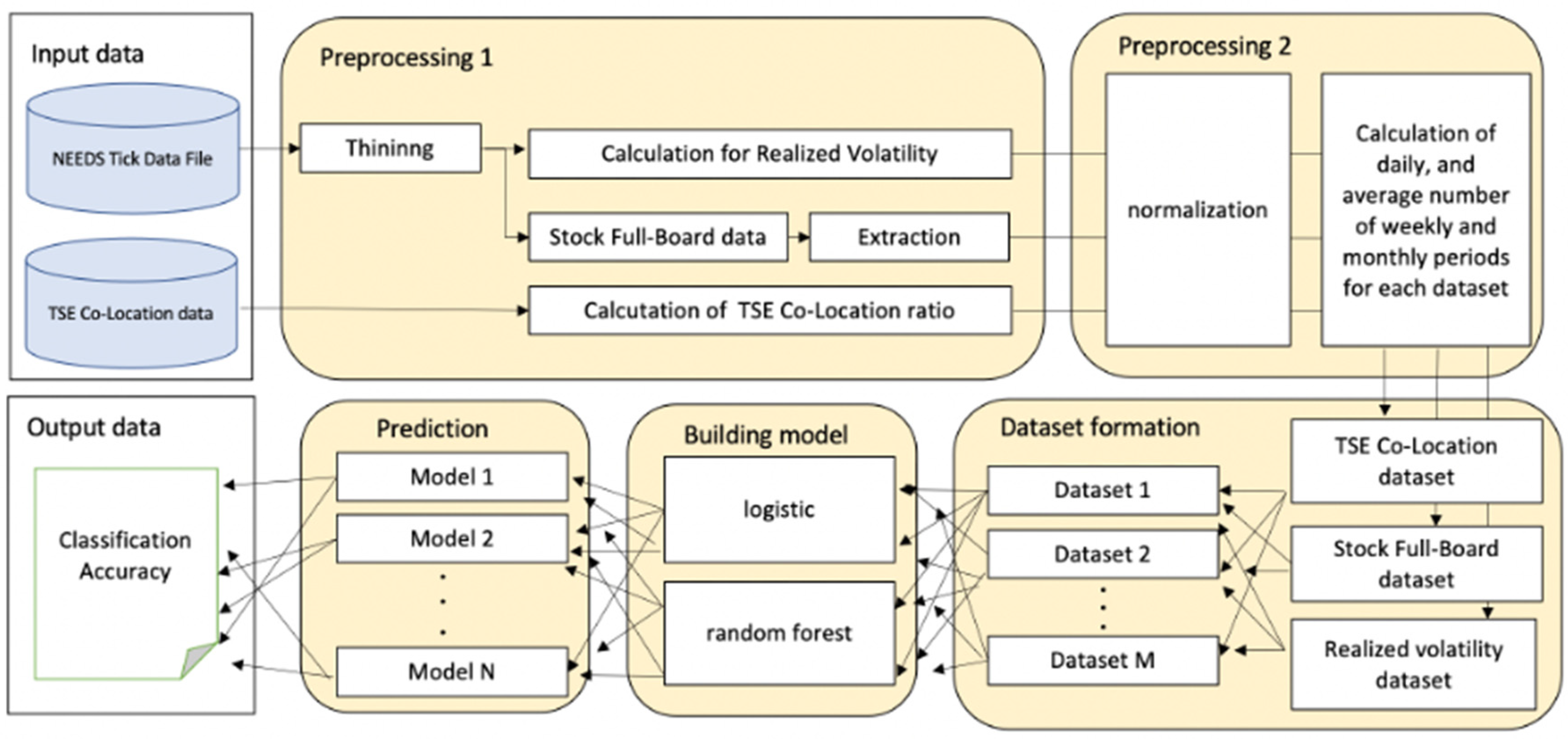
Figure 1 shows the entire process of the experimental procedure. First, we processed the raw datasets used in our research: NEEDS Tick Data File, which contains a stock full-board dataset and market volume dataset and the TSE Co-Location dataset, which contains HFT information. In preprocessing 1, the NEEDS Tick Data File, which is the high-frequency dataset, is thinned to reduce market micro-structured noise; then, we calculate RV and organize the stock full-board dataset. For the TSE Co-Location dataset, we calculate the ratio of all transactions traded from the TSE Co-Location server. By doing this preprocessing, we can determine the approximate effect of HFTs in the entire Japanese stock market. In preprocessing 2, we perform standardization so that different sizes of data can be analyzed in the same explanatory variable space. In addition, considering investors with various investment horizons, following the HAR model, we calculate the previous day data and the average of the past data (weekly and monthly, which correspond to 5 and 22 working days, respectively) for each variable to put in the explanatory space to predict RV.
In the dataset formation process, we created several combinations of explanatory variable datasets to analyze the contribution of each variable to the improvement of prediction accuracy.
Finally, we built models for each dataset using the logistic and random forest methods to compare their RV forecast accuracy. We provide the prediction accuracy from different methods and tasks. Below, we describe the details of each preprocessing and dataset.
3.1. NEEDS Tick Data File Preprocessing
We use the NEEDS Tick Data File provided by NIKKEI Media Marketing (
NIKKEI Media Marketing NEEDS Tick Data n.d.) for RV calculation (
Section 3.1.1) and stock full-board dataset preprocessing (
Section 3.1.2). Before calculation and preprocessing, we thin out every 5 min according to previous studies (
Ubukata and Watanabe 2014). Most previous researchers reported that the smaller the interval, the larger the market microstructure noise that may be contained during the RV calculation. We extract the following information: traded price, traded volume and stock full-board dataset, which is composed of the 1st best quote to the 10th best quote quantity and price on both the bid and offer sides. In the morning session, the data points we extracted were 09:01, 09:05, …, 11:25. In the afternoon session, 12:31, 12:35, …, 14:55. Note that there is only a morning session on both the grand opening and closing. Therefore, we extracted only the morning session on these two days.
3.1.1. Realized Volatility Calculation
Given return data
of intraday on
t, where
n is the sample size within a day,
RV is calculated by
where
Here, the subscript
t indexes the day, while
T indexes the endpoint within the observation period.
indexes the evening time-adjustment coefficient. The superscript (
d) in Equation (1) indexes daily. We follow
Watanabe (
2020) to calculate Equation (2), as proposed by
Hansen and Lunde (
2005). Note that we calculate the return for RV based on the trade price. If there are no transactions, we use the previously traded price.
3.1.2. Stock Full-Board Dataset Preprocessing
The stock full-board dataset is an important piece of information that provides valuable market conditions, such as the potential of market liquidity and the strength of demand and supply. These market conditions can affect volatility, which represents price fluctuation. In addition, a large bias in supply and demand suggests that the market is more likely to move in one direction (that is, a sign of a trend forming) and volatility may increase. This is well known from a practical point of view. Some previous studies use a stock full-board dataset to forecast returns or volatility in the Japanese market (
Toriumi et al. 2012).
When thinning out every 5 min, we follow the procedure below to extract information as explanatory variables from the stock full-board dataset. For each five min-period, we extract the 1st best quote to the 10th best quote quantity when either the price of the 1st best quote changes or is traded. Then, we take the summation of the 1st best quote to the 10th best quote quantity, standardized by the traded quantity. If there are no transactions, we use the previously traded price. Let
at the datapoint of t be the summation on both the bid side and offer side standardized quantity above. Then, we calculate using the following Equation: Suppose given data
and
.
Equation (3) describes the liquidity and Equation (4) describes the demand and supply of the market, respectively.
3.2. TSE Co-Location Dataset Preprocessing
The TSE Co-Location dataset (
Japan Exchange Group Connectivity Services 2021) is a new dataset that delivers HFTs trading information provided by the Japan Exchange Group. More specifically, it provides detailed information on HFT and is composed of order quantity, order to execution quantity and value traded quantity taken by the participants who trade via a server located in the TSE Co-Location area. This server only allows participants to perform HFT. In other words, the TSE Co-Location dataset is the aggregated information of transactions conducted through this server and this is the only dataset that can show the actual situation of HFT of stocks in Japan. Therefore, it is clear that the co-location information is closely related to high-frequency price data. Thus, it is an important variable that generates RV. As mentioned earlier, the importance of HFTs actions has been increasing annually since 2010. Under this trend, the TSE Co-Location dataset is the only important bridge for researchers and practitioners to consider the influence of HFTs in the Japanese stock market.
In this study, we use three explanatory variables on day t. Note that there are only two ways to trade Japanese stocks on the Tokyo Stock Exchange market: via TSE Co-Location or the other. Thus, each denominator of Equations (5)–(7) is the total number taken by these two methods. In contrast to the denominator, the numerator shows only the number taken through the TSE Co-Location server.
We also use the total value traded quantity as a single explanatory variable in our model, which is the denominator of Equation (7). This variable enables practitioners to understand a market activity or liquidity. It may be called the market volume data among practitioners. In this paper, we briefly describe this variable as follows.
3.3. Dataset Formation
We built five types of models: (I) HAR model, (II) HAR + Volume model, (III) HAR+ TSE Co-Location model, (IV) HAR+ Stock full board model and (V) HAR+ Volume + TSE Co-Location + Stock full board model, using the dataset mentioned in
Section 2.1 and
Section 2.2, as shown in
Table 1. As we mentioned in the overall process explanation, we prepare previous day data (which is denoted by “_daily”) and two different averages of past data, which are weekly and monthly (which is denoted by “_weekly” and “_monthly,” respectively), for each variable. By using these five different models, we examined how each variable contributes to the improvement of RV prediction accuracy.
Incidentally, the HAR model is known as the linear regression model in Equation (9),
where
This Equation is a linear combination of the constant term, daily
RV (which is denoted by
) calculated by Equations (1) and (2), weekly
RV and monthly
RV. Indicating the aggregation period as a superscript, the notation for the weekly
RV is
, while the monthly
RV is denoted by
. For instance, the weekly
RV at time
t is given by the average
The HAR model is not a long-term memory process but has three different types of autoregressive terms to approximate long-term memory processes.
As shown in
Table 1, we prepare different types of autoregressive terms for the explanatory variables. Note that these explanatory variables are the rate of change. Using these datasets, we build five different types of models and forecast the RV direction (“up” or “down”). For this, we define the RV direction as follows:
If
= 1, this case is omitted from the training dataset. In this study, there is no data point for this case.
3.4. Methods
Random forest is a popular machine learning method used for classification and regression tasks with high-dimensional data (
Breiman 2001). Random forests are applied in various areas, including computer vision, finance and bioinformatics, because they provide strong classification and regression performance. Random forest is called ensemble learning in the field of machine learning because random forest combines and aggregates several predictions outputted by several randomized decision trees. Each decision tree corresponds to a weak discriminator in ensemble learning. Random forests are structured through an ensemble of
d decision trees with the following algorithm:
Create subsets of training data with random sampling by bootstrap.
Train a decision tree for each subset of training data.
Choose the best split of a variable from only the randomly selected m variables at each node of the tree and derive the split function.
Repeat steps 1, 2 and 3 to produce d decision trees.
For test data, make predictions by voting or by averaging the most popular class among all of the output from the d decision trees.
The Gini index proposed by Economist Gini is a popular evaluation criterion for constructing decision trees (
Breiman et al. 1984), where the Gini index is used to measure the impurity of each node for the best split. The criteria of the best split are determined to maximize the decline rate of impurities at each node. The Gini index is an essential criterion for selecting the optimal splitting variable and the corresponding threshold value at each node. Suppose
is the number of pieces of information reaching node
n and
is the number of data points belonging to class
. The Gini index,
, of node
n is
A higher Gini index value for node n represents an impurity. Hence, a decreasing Gini index is an important criterion for node splitting.
While the random forest method is not state-of-the-art, such as deep learning techniques, we choose this method as it has several preferable features. First, random forests provide higher classification accuracy because they integrate a large number of decision trees. Second, random forests are robust to over-fitting because of the bootstrap sampling of data and random sampling of variables to build each decision tree; hence, the correlation between decision trees is low. As a result, the effect of overfitting is extremely small and the generalization ability is enhanced. Third, random forests can handle large datasets without needing too much calculation time because they enable researchers to train multiple trees efficiently in parallel. Moreover, unlike deep learning, the number of hyper-parameters is small and researchers do not need to puzzle over the hyper-parameter settings; researchers only need to choose the number of decision trees to build a model. Finally, random forests can be used to rank the importance of variables, which helps researchers identify the influential variables in the model. Therefore, researchers can manage the model efficiently and explain the contents of the model to stakeholders.
4. Experimental Results
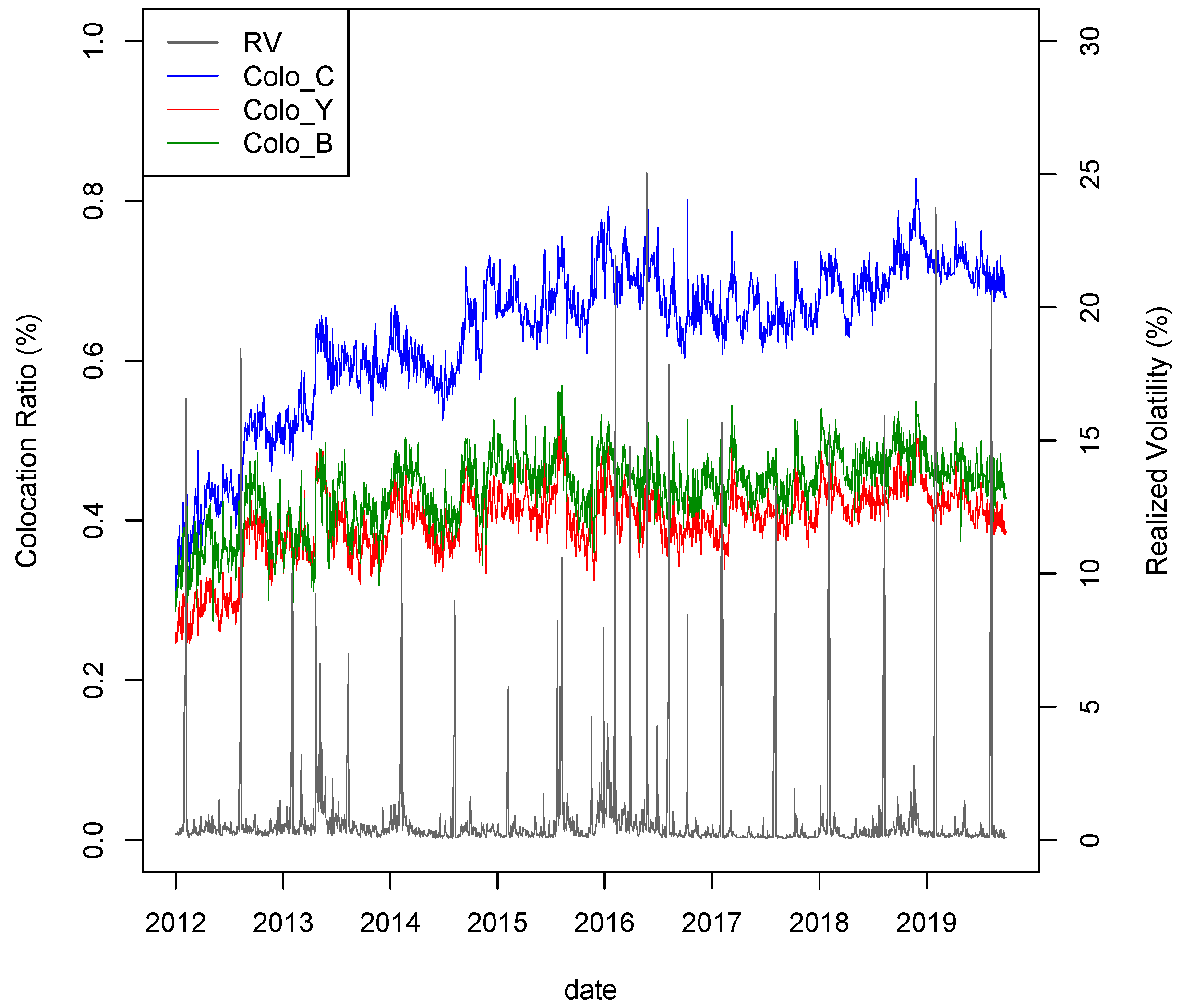
In this section, we present the experimental results. The TSE Co-Location dataset may not be familiar to both practitioners and researchers; hence, we show the time series chart of the TSE Co-Location dataset and RV in
Figure 2 and discuss its implications.
As can be seen from this figure, in the early 2010s, each TSE Co-Location index gradually increased because Arrowhead was introduced in 2010. This implies that the number of HFTs gradually increased during the system transition period. That is, the adjustment time to a new system varies from practitioner to practitioner. Thus, each index continues to increase for a certain period. A few years after its introduction, the Arrowhead system was revised in 2015. This revision allows trading participants to trade faster and more frequently. As a result, Colo_C continued to rise from the middle of the 2010s to the end of the 2010s. In contrast, Colo_B and Colo_Y have been flat since 2015.
As noted in the previous section, most HFTs in the Japanese stock market are foreign investors. Thus, we are of the opinion that these three TSE Co-Location numbers refer mainly to foreign investors. Since 2010, the Abenomics policy has attracted foreign investors’ interest in the Japanese stock market. It is known that foreign investors account for approximately 70% of the Japanese stock market (HFT and regular trading).
4.1. Observation Period
Our observation period is from 1 March 2012 to 31 October 2019. This period covers an essential event, that is, the renewal of Arrowhead on 24 September 2015. In addition, the beginning of our observation is not far from the implementation of the Arrowhead system. Namely, our observation period covers most of the period since HFT became possible in Japan. Thus, our examination of the accuracy of the model is highly reliable. We split the data into training data and test data with a 9:1 ratio. When building the model, we must consider data bias. If data are biased during the training period, the model is biased.
Table 2 shows the sample size of “up” and “down.” From
Table 2, our experimental result is worthy of discussion because there is no bias in the training data.
4.2. Experimental Results and Consideration
4.2.1. RV Prediction Accuracy
In this sub-sub section, we examine the different types of models by RV forecast accuracy and evaluate the effect of each dataset on the improvement of RV forecast accuracy through various experimental patterns. To evaluate the prediction accuracy, we used the F-measure, which is the harmonic mean that summarizes the effectiveness of precision and sensitivity in a single number. It is commonly used for evaluating the accuracy of classification (
Croft et al. 2010;
Patterson and Gibson 2017).
Here, precision measures the number of correct predictions divided by all instances. Sensitivity measures the number of correct predictions divided by all correct instances.
Table 3 shows the prediction accuracy of the RV during the total observation period for each model.
In the explanatory variables, the space of the HAR model (denoted as NoⅠin
Table 3; below, we unify this notation rule and others, as well), logistic method and our suggested random forest method yield almost the same prediction accuracy. However, with an increase in explanatory variables, the difference in prediction accuracy between the logistic method and the random forest method is larger. For instance, there is a 22% difference inaccuracy in the HAR + Volume + TSE Co-Location + Stock full-board model. These results are consistent with those of previous studies (
Ohlson 1980;
Shirata 2003;
Hastie et al. 2008;
Alpaydin 2014), which reported that linear models do not work where there are many explanatory variables in space.
Next, we shift to the differences between the models based on the RF method. The HAR model yielded a forecast accuracy of 60%. On the contrary, the HAR + Volume model yielded a 4% higher accuracy than the HAR model. In addition to the HAR + Volume model, the HAR + TSE Co-Location model and the HAR + stock full-board model yielded 3% and 6% higher accuracy, respectively. Moreover, the HAR + Volume + TSE Co-Location + Stock full-board model was 8% higher. From these results, it is evident that each explanatory variable helps the HAR model to improve forecast accuracy. In particular, the finding of an 8% increase in the prediction accuracy is a major contribution. However,
Table 3 implies that the features of these three variables may partially overlap. Compared to the total of 13%, which is simply the sum of the effects of each explanatory variable, the HAR + Volume + TSE Co-Location + Stock full-board model yields 5% lower than 13%. Future studies could work toward elucidating the aspects in which each variable has overlapping features despite having different data generating processes.
4.2.2. Analyzing Important Variables
The order of important variables helps us gain an in-depth understand and confirm the important variables. This information is especially beneficial for practitioners because they have to explain the content of the model to customers or supervisors. The random forest method generates the importance of each variable. This visualization is one of the advantages of the random forest method.
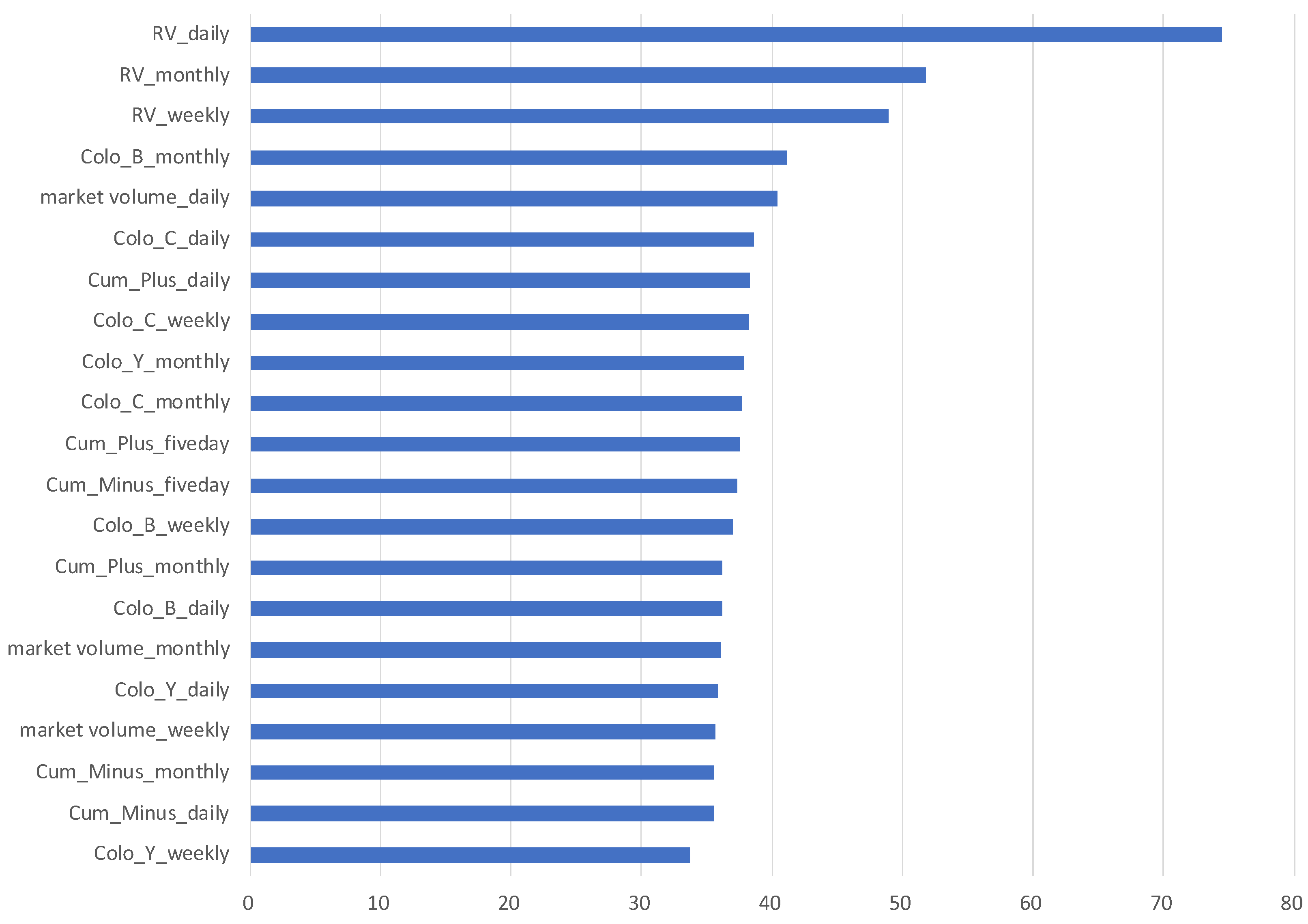
Figure 3 shows the importance variables arranged in descending order based on the Gini index in the building process of the HAR + Volume + TSE Co-Location + Stock full-board model. Thus, we know that RV_daily is the most important variable in this model. RV_monthly and RV_weekly are the second and third most important variables, respectively.
The top three important variables are RV’s autoregressive terms in different time horizons. This result is natural because there is a clustering effect on volatility. The RV’s past data are beneficial information for the forecast itself. Interestingly, five of the Top 10 important variables are the TSE Co-Location dataset. This accounts for over 70% of the Top 10 variables. We can state that the TSE Co-Location dataset is especially important for improving the prediction accuracy of the HAR + Volume + TSE Co-Location + Stock full-board model. Especially for Colo_C, all types of time horizons rank in. In contrast, for Colo_B and Colo_Y, the monthly time horizon is ranked. The results indicate that long-term trends are more important than short-term trends for these two variables. Market volume_daily and Cum_Plus_daily were also ranked in the Top 10 important variables. Both variables are related to market liquidity. The difference between the two variables is the amount actually traded or the amount that can be traded. As mentioned above, liquidity is closely related to volatility. Higher liquidity stabilizes the market environment, where prices are less likely to jump and volatility is more stable. This result is consistent with a practical point of view. Contrarily, the results of the importance of Cum_minus are rather surprising to practitioners. From a practical point of view, Cum_minus is known as an important variable in looking at the future direction of the market and indicates the strength of supply and demand between selling and buying. Our results suggest that the price direction may not be directly related to the up and down forecast of RV since the ranking of Cum_Minus_weekly, Cum_Minus_monthly and Cum_Minus_daily is not very high; they are ranked 12, 19 and 20 out of 21 variables, respectively, in the important variables.
From another perspective, we look at the important variables from the time horizon: daily, weekly and monthly.
Table 4 shows the rank of the periods in descending order by the Gini index for each category. In most categories, the daily period was ranked at the top. We cannot always necessarily say that the shorter the period, the more important it is. The comparison between weekly and monthly data is more important than weekly data. From this case, it is evident that very short periods and slightly longer periods play a more important role in the model. However, it depends on the category, but the tendency is as noted above. One possible explanation is that the expiration of information, which is aggregated by these categories, is nonlinear in RV forecast in the Japanese stock market. Detailed discussions require larger and more extensive analyses, such as comparing trends among countries.
4.2.3. Examination of TSE Co-Location Dataset Importance
To examine the effect of the TSE Co-Location, we split the total observation period (1 March 2012 to 31 October 2019) into two periods to consider the effect of Arrowhead renewal in 2015: the first half period (1 March 2012 to 23 September 2015) and the second half period (24 September 2015 to 31 October 2019). For each period, we build a model in the same framework as in the previous sub-sub section to compare the differences in important variables between the first and second half periods from a time-series perspective.
Figure 4 and
Figure 5 show the important variables in the first and second half periods, sorted in descending order based on each period. Considering the changes in the importance of variables, RV remains an important variable in both the first and second half periods. However, in the categories excluding RV, the importance of the TSE Co-Location dataset increased overall and ranked higher from the first half period to the second half period. In particular, the increase in Colo_C was remarkable. Colo_C occupies the second position in the second half period, following RV. Colo_B ranks in the top three, but this category is less important in the TSE Co-Location dataset than in the first half period. This suggests that information on the order status of HFT among market participants is more valuable than that of what is bought or sold. It is interesting to recognize this trend as an increase in HFTs. In contrast, Colo_Y was not as important in both periods. In fact, remember the flow of order → execution → trading volume, when an order is filled, that number is reflected in the trading volume. From this, we think that it is possible to interpret that Colo_Y is not an important variable because it has a strong meaning between order and trading volume.
We consider other interpretations in this regard. Since the beginning of Arrowhead, the proportion of HFTs in the Japanese stock market has been on the rise and the transition period is thought to have continued until around 2015. For instance, all the variables in
Figure 2 from 2010 to 2015 are in an uptrend. In contrast, in the second half of the period, the patterns of these variables changed. Colo_C continued to increase after 2015. This is because system renewal helps market participants to place orders more quickly. Thus, the importance of Colo_C increased during the second half period. Except for Colo_C, the others only move within this range. Although the quality of each variable may charge slightly more or less due to the effect of the Arrowhead system revision in 2015, the effect should not be as large as before and after the implementation of Arrowhead in 2010. As seen in
Figure 2, the system revision in 2015 was not enough to generate a trend in Colo_B and Colo_Y. Therefore, these two TSE Co-Location variables may be less important in the second half period.
On the whole, the importance of our proposed datasets and the method of its usage, which describes the summary of the data generating process in HFT, has been increasing in proportion to the increase in the importance and participants of HFT. As evident from
Table 5, the HAR + Volume + TSE Co-Location + Stock full-board model in the second half period yields a 5% higher forecast accuracy.
Table 6 shows the sample size of the training and test data for each period used in this analysis.
Regarding other variables, it was found that the importance of market volume has decreased and Cum_minus, which observes the changes in supply and demand, has become more important. Although this is a different result from that in the previous subsection, it goes without saying that the results will change depending on the analysis period.
5. Discussion and Conclusions
This study suggests a new approach for RV forecasts of TOPIX futures. The characteristic of our model is that it uses not only the HAR dataset but also the TSE Co-Location dataset and stock full-board dataset, both of which are related to HFT and the market volume dataset based on the random forest method. We showed that our model yields a 9% higher prediction accuracy compared to the HAR model based on the logistic method in the total observation period. In addition to this novel high accuracy, we found that the TSE Co-Location dataset, which contains HFT information, tends to play a more important role and affects daily RV forecasts. This finding is consistent with the previous studies (
Zhang 2010;
Haldane 2011;
Benos and Sagade 2012;
Caivano 2015;
Myers and Gerig 2015;
Kirilenko et al. 2017;
Malceniece et al. 2019). In addition, this implies that transactions in high-frequency regions have an effect on economic agents who conduct transactions at a low frequency. High-frequency data are generally considered to be used only for HFT, but we have shown that it is also beneficial to the general frequency area.
These results indicate that our proposed datasets contribute to the increase in the accuracy of prediction and have a high affinity with the random forest method. The random forest method excels in prediction accuracy compared with the logistic model on average, as we expected, corresponding to the model accuracy in the previous section. Regarding this point, we consider that it is natural and consistent with previous research (
Tanaka et al. 2018a;
Tanaka et al. 2019), which have similar frameworks. As noted in the previous section, linear models do not work in the large explanatory variable space. In fact, from
Table 3, it is evident that the logistic method seems to overfit. Practitioners and researchers should select nonlinear methods, such as the random forest method. The quality of the Japanese stock market changed due to the introduction of Arrowhead in 2010 and the effect continued strongly. Moreover, we found important rolls of the TSE Co-Location dataset deeply related to RV. We consider that the dataset associated with HFT, such as the TSE Co-Location dataset, is expected to play an important role in the model building process with the upcoming revolutions in trading systems. Now, we cannot evade high-dimensional explanatory space by adding a new dataset to the HAR. We propose the use of new datasets. By combining them with the random forest method, we show novel experimental results regarding RV forecast during two crucial events: the introduction and revision of Arrowhead. Overall, our proposed model is superior to the HAR model and can be expected to yield a high prediction accuracy. If there is a similar dataset to the TSE Co-Location dataset, our framework can be applied to the other stock markets as well.
Nevertheless, the forecasting problem may vary depending on conditions such as the selection of sampling periods. In particular, when the quality of the market changes due to new regulations, even if the model has a high accuracy of forecast in the past, in some cases, it may be necessary to revise the model in anticipation of the upcoming data in the near future. In such cases, practitioners will need to search for similar events in history, grasp the strengths and weaknesses of pattern recognition of the dataset at that time and correct them. Despite the model yielding a high prediction accuracy during the training period, it can be completely useless during the test period. Dividing the sample period appropriately, which is a universal problem, is an issue in this study. In future work, we would like to find a way to divide it automatically and conveniently.
There are pros and cons to HFT not only in Japan but also globally.
Linton and Mahmoodzadeh (
2018) indicate that fast algorithmic transactions place unexpectedly large orders due to program errors and algorithms that behave differently than the programmer tend to cause chain reactions, increase market volatility and disrupt market order (For instance, the May 2010 Flash Crash, August 2012 wrong order by Night Capital, October 2018 Tokyo Stock Exchange Markets Arrowhead system trouble triggered by Merrill Lynch, September 2020 Tokyo Stock Exchange Markets Arrowhead system trouble and so on). On the contrary, IOSCO reports that there is a close relationship between liquidity and volatility, in the sense that more liquidity can better absorb shocks to stock prices. HFT involved in official market-making businesses may help mitigate volatility in the short hours of the day by providing liquidity. In fact, HFT is thought to be responsible for more than 40% of the trading volume in the Japanese equity market in 2019, as shown in
Figure 2. From the perspective of market liquidity and pursuit of alpha by hedge funds through HFT, we consider that HFT will play a more important role in any case. Our proposed dataset contributes to improving prediction accuracy through various types of experiments. We have experimentally shown that the degree of influence has increased in recent years. We believe that this trend will intensify in the future. Recently, the Financial Services Agency of Japan has been strengthening monitoring and legal systems, such as requiring frequent registration to trade. Along with this, the environment of HFT in the Japanese stock market is getting better, with further system improvement efforts by the Tokyo Stock Exchange, development of private exchanges and dark pools in securities firms and upgrade of securities firm systems to connect customers and securities firms more quickly.
In future work, we would like to examine this in more detail by decomposing the effect of each variable on the RV forecast improvement. Furthermore, considering
Baillie et al. (
2019), there may be room to extend our model, taking into account the long memory process.
Chen et al. (
2018) and
Ma et al. (
2019) are one of the helpful existing researches to expand our random forest based model to integrate long short-term memory process. In addition, we would like to extend our framework to higher-order moments. High-order moments are an important research area in finance.
Hollstein and Prokopczuk (
2018) showed that volatility affects stock returns.
Amaya et al. (
2015) insist that high-order moments are beneficial information for asset price modeling. Hence, we believe that verifying the effectiveness of our approach even in high-order moments would be helpful for both practitioners and researchers.


