Abstract
Financial data are expensive and highly sensitive with limited access. We aim to generate abundant datasets given the original prices while preserving the original statistical features. We introduce the Wasserstein Generative Adversarial Network with Gradient Penalty (WGAN-GP) into the field of the stock market, futures market and cryptocurrency market. We train our model on various datasets, including the Hong Kong stock market, Hang Seng Index Composite stocks, precious metal futures contracts listed on the Chicago Mercantile Exchange and Japan Exchange Group, and cryptocurrency spots and perpetual contracts on Binance at various minute-level intervals. We quantify the difference of generated results (836,280 data points) and original data by MAE, MSE, RMSE and K-S distances. Results show that WGAN-GP can simulate assets prices and show the potential of a market simulator for trading analysis. We might be the first to look into multi-asset classes in a systematic approach with minute intervals across stocks, futures and cryptocurrency markets. We also contribute to quantitative analysis methodology for generated and original price data quality.
1. Introduction
Various scholars are trying to solve price prediction problems to capture short-term alphas in the markets (Ariyo et al. (2014); Foster (2002); Abraham et al. (2018)). However, a more fundamental contribution can be understanding the underlying price behavior of multiple asset classes with limited data. One of the critical processes is to generate enough data for observations and backtesting, therefore we want to learn the distribution of asset prices based on limited price information. We hope to generate richer varieties of data to simulate the original prices while preserving the original statistical features. Stock prices are considered to be random walks (and crypto as well) by Palamalai et al. (2021). To simulate the price behaviors, we adopt WGAN-GP to generate richer data with noise to discover hidden characteristics. To ensure the quality of generated real and fake data discriminated by WGAN-GP, we use MAE, MSE, RMSE and KS distance to calculate the price differences with multiple minute level intervals.
The Generative Adversarial Network(GAN) Goodfellow et al. (2014)’s success in generating realistic synthetic images has inspired machine learning for generating multi-asset class prices. The GAN models in image generations could be used in financial datasets. Inspired by the generator and discriminator ideas, we implement a Wasserstein GAN with Gradient Penalty (WGAN-GP) framework to learn the underlying original financial datasets distributions, given minute level intervals prices across stocks, futures and cryptocurrencies markets. We explore a universal WGAN-GP model to simulate multi-asset classes datasets purchased from the Hong Kong Stock Exchanges, the Chicago Mercantile Exchange and the Japan Exchange Group. We report observations from stocks, futures and crypto markets, and evaluate generated prices against original datasets. The results showed good performance, and we can use WGAN-GP as a probabilistic prediction model on financial time series to obtain the potential distribution of original financial datasets.
Since financial datasets contain potentially sensitive information, datasets are always headaches for quantitative researchers for predictive purposes when backtesting algorithm trading strategies ranging from multiple time intervals like intraday and high frequency trading. Furthermore, based on abundant prices, reducing algorithm overfitting and enhancing the robustness of portfolios when markets are volatile are desired among professional users. Moreover, stock datasets have unique features like ‘tick size’ and trading mechanisms for each market including auctions and continuous trading sessions, while futures contracts have day and night sessions.
Here, we propose a practical model focusing on minute-level prices and quantifying the quality against original prices. Li et al. (2020) obtained the training tick data from OneMarketData as a financial data provider. Samuel et al. (2021) trained the WGAN-GP for daily prices downloaded from Yahoo Finance (n.d.)1, but generated data are distinguishable. Their WGAN-GP consists of a generator and discriminator function which utilize an LSTM architecture. However, the model has space for optimization, which could be achieved by adjusting the hyperparameters. One of the solutions could be the learning rates. Samuel used an RMSprop optimizer with a fixed learning rate of 0.00005. Smith (2017) proposed training with cyclical learning rates instead of fixed values, which achieves improved classification accuracy. WGAN-GP can be trained to customize conditions through parameter settings like cyclic learning rates. To ensure the input data quality, we purchased all limit order books data including trades and order books from HKEX for stocks and CME and JPX for precious metals. We downloaded cryptos spots and perpetual futures from Binance, one of the biggest exchanges. To the best of authors’ knowledge, we might be the first to look into multi-asset classes in a systematic approach with minute-level intervals observations with WGAN as in Figure 1.
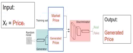
Figure 1.
Given the original market prices as input, we trained the datasets using WGAN-GP and output the generated real and fake prices judged by the discriminators. The generator struggles to trick the Discriminator, while the Discriminator criticizes the generator until approaching equilibrium, keeping the training process as a zero-sum game in Algorithm 1.
We propose the following research questions:
- Can WGAN-GP be trained as a probabilistic model for financial prices simulations?
- Can WGAN-GP simulate multiple minute-level intervals prices?
- How good are the WGAN-GP when simulating multiple asset classes, e.g., stocks, futures and cryptos?
The contents are organized as follows. Section 2 describes the model GAN, WGAN and WGAN-GP with their features. Section 3 describes our proposed model based on WGAN-GP and multiple asset classes datasets. Section 4 includes the results for training the Hong Kong stocks. Section 5 reports the performance of precious metal futures including gold CME Gold Futures and Option (n.d.), JPX Gold Futures and Options (n.d.) and platinum CME Platinum Futures and Options (n.d.), JPX Platinum Futures and Options (n.d.) futures products listed on CME and JPX. Section 6 focuses on training cryptocurrencies including spot and perpetual futures contracts. Section 7 discusses the results and provides implications for future research. Finally, we conclude our model performance and give insights about multi-asset classes simulations in Section 8.
| Algorithm 1: WGAN-GP algorithm |
| for do |
| for do |
| sample ; |
| sample ; |
| ; |
| ; |
| ; |
| end for |
| sample batch noise again; |
| ; |
| CyclicLR(epoch, , ; |
| end for |
Algorithm 1 WGAN-GP trains each asset class with customized parameters, and we systematically examine the difference between generated data prices and original prices by MAE, MSE, RMSE and KS test in Section 4 for stocks markets, Section 5 for precious metal futures listed on CME and JPX and Section 6 for cryptos listed on Binance including spots and perpetual futures.
2. Generative Adversarial Networks
Generative adversarial networks are unsupervised learning algorithms that build two neural networks competing in a zero-sum game. The ultimate goal of GAN is to generate close to original distribution . Using GANs on images is easy and intuitive, however hard for humans to examine large-scale datasets.
2.1. GAN Structure
Generator and discriminator are the two models in a game playing against each other during the training. The generator will output an image initiated from random noise and pass it to the discriminator as a binary classifier assigning generated real or fake labels. The generator struggles to adjust according to the feedback and continues to fool the discriminator. Meanwhile, the discriminator continues to refine the decision making strategies until it cannot differentiate real and fake ones. The optimal states of the discriminator are random guesses with 0.5 accuracies.
2.2. GAN Training
The GAN has iterative gradient descent for both players. The Loss function is obtained by taking a batch of real (from ) and generated samples (from = ). ADAM or RMSprop optimizer is widely used for increasing training convergence. The overall value function Value (G, D), which incorporates both Loss(D) and Loss(G), is defined as:
Both players can be lazy from updating, leading to mode collapse, ignoring all other modes and staying in the comfort zones with few states. The generator can only create a few generated data when minimizing the loss while Discriminator remains passive feedback.
2.3. Wasserstein GAN
Wasserstein GAN solves the mode collapse problems by subtle changes on the models with earthmoving distance by Arjovsky et al. (2017). However, weight clipping is hard to enforce a Lipschitz constraint to stabilize the training while keeping diversified data varieties.
2.4. Wasserstein GAN with Gradient Penalty
A derivable function is 1-Lipschtiz if and only if it has gradients of norm at most 1 everywhere. Therefore, the gradient penalty is used to constrain the gradient norm of the critic’s output to be 1 everywhere in regard to its input. The gradient penalty by Gulrajani et al. (2017) is added to the objective:
3. Our Proposed Model and Asset Classes Datasets Descriptions for Training
We initialize , , , , , . We used an AMD EPYC 7H12 64-Core Processor 2.6 GHz, with 1 TB RAM, and 4 Nvidia A100-SXM4-40 GB GPUs for the training tasks, since each dataset is pretty big with all limit order books information, the powerful server can better model the training performance. The training takes around 200 h to complete, and generate a total of 836,280 data points, 4140 data points for each row, respectively. For stocks we generated 372,600 points for HSI Composite, 115,920 data points including TGD, TPL, PLE and GCE for precious metal futures, 202,860 for cryptos spots and 144,900 for crypto perpetual futures. The parameters for training are outlined in Table 1 and multiple asset classes datasets in Table 2.

Table 1.
Parameters settings for WGAN-GP, a combination of different parameter settings, can approach the optimal loss efficiently. We outlined the parameters for training considerations.
Table 2.
We systematically examined the multiple asset classes, including shares (HSI Composite Stocks), futures (Gold, Platinum Futures on CME and JPX) and cryptos (Spot, Perpetual contracts). The data was purchased directly from the exchanges and was of the highest quality.
For the Hong Kong market, Kim and Mei (2001) showed that political developments in Hong Kong have a significant impact on its market volatility and return. The extended ARCH-jump filter with bad news has a more significant volatility effect than good news. The unique characteristics can be price jumps that misprice derivative products tracking benchmark HSI indices, leading to a dynamic hedging portfolio less effective with jumps caused by policy risks. Xu et al. (2020) argued market liberalization leads to lower quoted spread, lower effective spread, lower market depth, and higher short-term volatility for the Shanghai–Hong Kong Stock Connect program (SHHKConnect). Meyer and Guernsey (2017) discussed how high frequency trading on the HKEx compared to the SGX may derive from an underlying conflicted approach within Hong Kong’s political-economy about how HKEx relates to China’s exchanges. On this occasion, we might be the first to look into the Hang Seng Index Component Stocks, a total of 60 stocks. We introduce WGAN into Hong Kong stocks simulations to better understand Hong Kong markets.
For the futures market, Kang et al. (2017) evaluated and compared optimal portfolio weights and time-varying hedge ratios from 4 January 2002 to 28 July 2016. They showed directional spillovers (DS) could transmit from one market to another. Xu and Fung (2005) indicated that pricing transmissions for these precious metals contracts are strong across the two markets. Still, information flows appear to lead from the U.S. market to the Japanese market in terms of returns, and the offshore trading information can be absorbed in 24 h. Mensi et al. (2021) suggested that gold and silver are net contributors of risk to the other markets, whereas palladium is a net receiver of risk for all the time horizons. Platinum is a net contributor of risk to the other markets in the short term and a net receiver of risk from the remaining markets in the intermediate- and long-term horizons. Precious metals provide diversification gains to currency investors for all time horizons.
For the cryptocurrency market, Lee et al. (2020) studied BTC data from January 2018 contracts to March 2019 on all CBOE and CME. They concluded that Bitcoin spot and futures are cointegrated, and Bitcoin futures are biased predictors of spot prices. Kyriazis et al. (2019) studied bearish market daily data from 1 January 2018 to 16 September 2018. They concluded that the highest capitalization digital currencies, namely Bitcoin, Ethereum and Ripple, will influence others. Baur and Hoang (2021) concluded stablecoins are relatively safe compared with BTC. We benchmarked BTC as the highest market capitalization asset from the above literature.
4. HANG SENG INDEX Components Stocks Simulations
The Hang Seng Index (HSI) is the main stock market index in Hong Kong to monitor the daily changes of the largest companies listed in the Hong Kong stock market. HSI is the leading indicator of the overall market performance in Hong Kong. These 60 constituent companies represent about half of the capitalisation of the Hong Kong Stock Exchange.
4.1. Data Cleaning for HKEX Datasets
The complete limit order book and trade book data were purchased from HKEX. After deserializing from binary files into MongoDB to reconstruct simulations, we recorded the stock code and order book modification, including cancellation and trade orders in milliseconds. To generate an order book snapshot, we resampled by consecutive trading minutes to obtain Open, Close, High and Low prices. Finally, we obtained the minute-level original Close prices.
4.2. Input and Output Prices for the WGAN-GP Model
Here, we introduced the input prices of original minute close in Figure 2 for WuXi Biologics 2269.HK as an example and output as generated minute close prices in Figure 3, followed by density plot by price distributions in Figure 4 for 2269.HK.
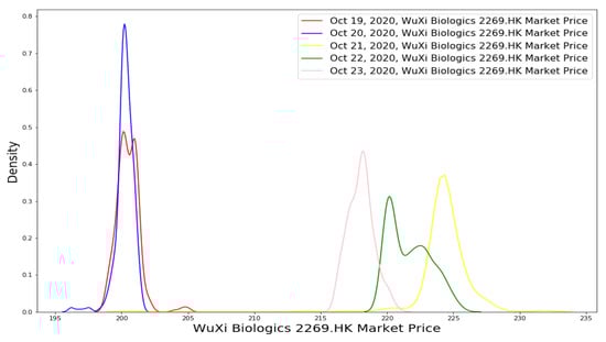
Figure 2.
WuXi Biologics is a listed company on the Hong Kong Stock Exchange, one of HSI Composites. For a consecutive trading week, the prices at minute level intervals are plotted in six distributions (the total area under the curve integrates to one with each date as one distribution). The probability density (Y-axis) is the per unit on the prices (X-axis). There exist statistics properties like kurtosis and skewness, mean and standard deviations.
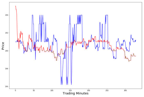
Figure 3.
Generated real price at the minute interval (blue) and original market close prices (red) are plotted for 2269.HK. Starting from the first minute, the auction period will impact the following several trading minutes. The generated real prices are pretty close to the original input, as shown in tick movement.
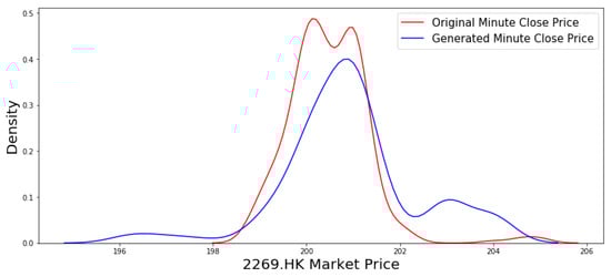
Figure 4.
After mapping the price information by price, the generated prices (blue) are compared with one-minute market close prices (red).
Given the price distributions at minute intervals for 2269.HK, we started from 19 October 2020, and fed the minute interval prices into the WGAN-GP model. The generator tries to fool the discriminator by generating as many data points as possible. In contrast, the discriminator struggles to judge by labelling real and fake compared to the original data.
After obtaining the generated real data, the two curves can be plotted in the same graph (the X-axis is the price). The simulated real price curve is twisted around the original minute level close. We need to quantify the difference between two prices by MAE, MSE, RMSE and K-S distances Table 3. As shown in Table 3 and Table 4, we calculated and generated 19–23 October 2020, five trading days with MAE-R, MSE-R and RMSE-R, where R denotes Generated Real, meaning the differences against original input minute close prices. To further ensure the quality of generated real and fake data, we investigate the KS test with Generated Real and Fake compared with original input prices. Usually, the smaller KS, the better results. The KS R/F ratio means the difference between KS Real and KS Fake. Similarly, the smaller, the better.
Table 3.
We listed the performance of our model by MAE-R, MSE-R, RMSE-R, and KS tests.HSI Composite stocks are grouped by tick.
Table 4.
We selected several typical stocks at different tick values and reported the performance of our model at one, two, three, four, five, ten and fifteen minute intervals. Tick values include 0.2, 0.1, 0.02, 0.05 and 0.01. 2269.HK-15 min in Table 4 shows highest MAE-R/ Tick in all minute intervals compared with other selected representatives by ticks.
Hong Kong securities market includes 1. Auction Session Pre-opening Session 9:00 a.m.–9:30 a.m. 2. Continuous Trading Session from 9:30 a.m. to 4:00 p.m. with an hour break in the noon Hong Kong Exchanges and Clearing Limited (n.d.). HSBC continuous trading minutes include pre-opening session and continuous trading session with an closing auction every market open day shown in Figure 5.
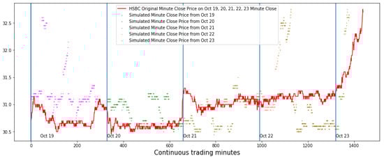
Figure 5.
For the consecutive trading minutes from 19 October to 23 October 2021, we plotted the minutes trading level (X-axis) and minute interval close prices (color red), with the simulated/generated prices in other colours. The open market auction impacts the morning continuous trading session after 9:30 a.m. And starting from 3:30 p.m., there exists market impact caused by China Connect until market close.
4.3. Quantitative Results by MAE, MSE, RMSE, K-S Tests, KS R/F Ratio and MAE-R/ Tick
We measured the difference by mean absolute error (MAE), mean squared error (MSE), and root-mean-square deviation (RMSE). Due to the page limit, we only listed Generated Real data with original market close data. We calculated the Kolmogorov-Smirnov test (KS-test) between Generated Real and Generated Fake to quantify the distribution difference with original market close price data.
MAE represents the difference between the real and fake values extracted by averaging the absolute difference over the datasets. MSE represents the difference between the real and fake values extracted by squaring the average difference over the dataset.
where denotes real values and denotes fake values.
The KS-test is a kind of “goodness-of-fit test”. Suppose that we have an i.i.d. sample with some unknown distribution and we want to test the hypothesis that is equal to a particular distribution , i.e., decide between the following hypotheses:
The KS-test tries to determine if two datasets differ significantly. The KS-test has the advantage of not assuming the distribution of data Li et al. (2020). Li et al. proposed model Stock-GAN outperformed against recurrent conditional variational auto-encoder (VAE) and DCGAN instead of WGAN. However, they only tested the model on two stocks: a large capitalization stock, Alphabet Inc (GOOG), on one trading day in August 2017 and a small-capitalization stock, Patriot National (PN), which has relatively poor performance. The Stock-GAN model KS distance is 0.126 for GOOG, which is better than VAE (0.218) and DCGAN (0.181).
4.4. Discussion for HANG SENG INDEX Components Stocks Markets
After rounding by tick size, the MAE-R/Tick can be referred as part of volatility. In Table 3, 1211.HK (Tick value = 0.2, MAE-R/Tick = 33.08), 2313.HK (Tick value = 0.1, MAE-R/Tick = 29.12), 2331.HK (Tick value = 0.05, MAE-R/Tick = 26.56), 1928.HK (Tick value = 0.02, MAE-R/Tick = 37.7), 0762.HK (Tick value = 0.01, MAE-R/Tick = 23.8) shows higher volatility in one minute interval. The highest KS REAL and KS FAKE are 0.122, 0.110 and the highest KS R/F Ratio is 1.519. Overall, the quantitative results show the WGAN-GP generated data for prices are of high quality.
5. CME and JPX Precious Metal Futures Market Simulations
The Chicago Mercantile Exchange and the Japan Exchange Group are among the most significant futures exchanges globally. Precious metals futures are the most liquid products. Gold, silver, platinum and palladium are precious metal commodities with a wide range of industrial usage. The precious metal also retains a significant role as a relatively stable investment instrument by the private firms, governments, LBMA and central banks. Precious metal futures are highly leveraged investments for hedging and speculations where margin can keep with broker or exchange.
We purchased the historical data on the website of CME Group and Japan Exchange Group covering the whole year of 2020 trade and order books. After resampling, we obtained Open, High, Low and Close at different time intervals.
5.1. Results on Japan Exchange Group Precious Metal Futures at Different Time Intervals
We selected 6 Janiary 2020, as our observation date, where we captured input prices at various minute intervals. Surprisingly, platinum futures at 15 min intervals have the least MAE-R. We generated 57,960 data points for TGD in Table 5 and TPL in Table 6 for a single day, at least three times larger than the original inputs.
Table 5.
TGD-n mins (TOCOM gold) represent futures contracts listed in JPX at one, two, three, four, five, ten and fifteen minutes intervals. For KS R/F Ratio, all are smaller than one, where the highest KS REAL and FAKE are 0.077 and 0.144. Precious futures contract tick value is all one dollar.
Table 6.
TPL-n mins (TOCOM platinum) represent futures contracts listed in JPX at one, two, three, four, five, ten and fifteen minutes intervals. For KS R/F Ratio, 2 out of 7 are bigger than one, where the highest KS REAL and FAKE are 0.138 and 0.143.
5.2. Results on Chicago Mercantile Exchange Precious Metal Futures at Different Time Intervals
Platinum futures have the highest MAE-R among all contracts, whether CME or JPX. We selected 6 January 2020, as our observation date, where we captured input prices at various minute intervals. We generated 57,960 data points for PLE in Table 7 and GCE in Table 8 for a single day, at least three times larger than the original inputs. We visualized Platinum futures contract (PLE) 15 minutes results in Figure 6.
Table 7.
PLE-n mins (platinum) represent futures contracts listed on CME at one, two, three, four, five, ten and fifteen minute intervals. Platinum futures have the highest MAE-R among all futures contracts. For KS R/F Ratio, two out of seven are bigger than one, where the highest KS REAL and FAKE are 0.193 and 0.188.
Table 8.
GCE-n mins (gold) represent futures contracts (CME) at intervals of one, two, three, four, five, ten, and fifteen. For KS R/F Ratio, all are smaller than one, where the highest KS REAL and FAKE are 0.058 and 0.145.
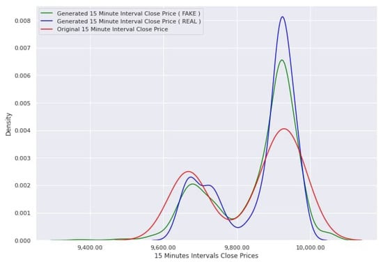
Figure 6.
Platinum futures contract (PLE) 15 minutes interval has a larger MAE-R 140.385 than other contracts. Price is concentrated in a certain range and generated long-tailed prices can represent more abundant prices than the original prices.
6. Cryptocurrencies Simulations
The cryptocurrency market runs continuously all day globally. The centralized exchanges across time zones are active somewhere at any time. A cryptocurrency is a digital currency secured by cryptography, making it nearly impossible to counterfeit or double-spend. Many cryptocurrencies are decentralized networks based on blockchain technology—a distributed ledger enforced by computers networks. As an emerging asset class, we examine the following spots and perpetual futures contracts by minute level intervals.
6.1. Spot Results and Analysis
A Spot Market is a market where investors can trade assets with other traders in real-time. As the name suggests, transactions are settled immediately or “on the spot” when the buying/selling order is filled. You can purchase an asset with fiat or another cryptocurrency from a seller as a buyer.
The data is open-source on the website of Binance (n.d.)2 where we downloaded spot and results for Bitcoin (BTCUSDT) in Table 9, Ethereum (ETHUSDT) in Table 10, Binance Coin (BNBUSDT) in Table 11, Cardano (ADAUSDT) in Table 12, Solana (SOLUSDT) in Table 13, XRP (XRPUSDT) in Table 14, Polkadot (DOTUSDT) in Table 15 on the date of 3 Septemper 2021, from 12:00 a.m. to 11:59 p.m. for a total of 1440 trading minutes. We generated 202,860 data points in total for a single trading day, 28,980 each symbol.
Table 9.
We examined BTC spot prices against generated prices at intervals of one, two, three, four, five, ten and fifteen minutes. For the KS R/F Ratio, four out of seven are more significant than one, indicating hard to train, where the highest KS REAL and FAKE are 0.112 and 0.114.
Table 10.
We examined ETH spot prices against generated prices at intervals of one, two, three, four, five, ten and fifteen minutes. For KS R/F Ratio, 2 out of 7 are bigger than one, where the highest KS REAL and FAKE are 0.094 and 0.186.
Table 11.
We examined BNBUSDT spot prices against generated prices at one, two, three, four, five, ten and fifteen minute intervals. For the KS R/F Ratio, two out of seven are more significant than one, where the highest KS REAL and FAKE are 0.103 and 0.113.
Table 12.
We examined ADAUSDT spot prices against generated prices at one, two, three, four, five, ten and fifteen minute intervals. For KS R/F Ratio, two out of seven are more significant than one, where the highest KS REAL and FAKE are 0.108 and 0.101.
Table 13.
We examined SOLUSDT spot prices against generated prices at one, two, three, four, five, ten and fifteen minute intervals. For KS R/F Ratio, three out of seven are bigger than one, where the highest KS REAL and FAKE are 0.082 and 0.073.
Table 14.
We examined XRPUSDT spot prices against generated prices at one, two, three, four, five, ten and fifteen minute intervals. For KS R/F Ratio, two out of seven are more significant than one, where the highest KS REAL and FAKE are 0.092 and 0.124.
Table 15.
We compared DOTUSDT spot prices against generated prices at intervals of one, two, three, four, five, ten, and fifteen minute intervals. DOTUSDT 15 minutes KS are the largest among all time intervals.
6.2. Perpetual Futures Results and Analysis
Perpetual contracts are derivative contracts similar to futures with no expiration date or settlement, allowing them to be held or traded for a consistent trading time. Perpetual contracts are gaining popularity in cryptos because they allow traders to hold leveraged positions without the burden of an expiration date. Unlike traditional futures, perpetual contracts trade close to the index price of the underlying asset due to perpetual funding rates. We included BTCUSDT Perpetual in Table 16 and visualized BTC Perpetual in Figure 7, ETHUSDT Perpetual in Table 17, BNBUSDT Perpetual in Table 18, ADAUSDT Perpetual in Table 19, and XRPUSDT Perpetual in Table 20 for multiple intervals.
Table 16.
We compared BTCUSDT perpetual prices at multiple time intervals. BTCUSDT at one minute interval has the highest MAE-R scores. The smallest KS REAL and KS FAKE are 0.044, and 0.071. The highest KS REAL and KS FAKE are 0.113 and 0.192, respectively.
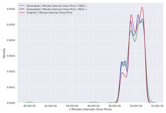
Figure 7.
This graph shows the BTC one minute Interval Close prices and generated fake and real price data. BTC perpetual futures contracts are relatively volatile, with a relative large MAE of 72,840.8 compared with other perpetual contracts. The highest density from the original reaches 0.0006. The long tails from generated real and fake show the potential price volatility indicated by the original prices covering 40,000 to 48,000 USDT.
Table 17.
We compared ETHUSDT perpetual prices at multiple intervals. The smallest KS REAL and KS FAKE are 0.029, and 0.054. The highest KS REAL and KS FAKE are 0.085 and 0.219 respectively. ETHUSDT perpetual 15 min intervals, KS R/F Ratio is 0.388 where KS REAL is 0.085, indicating the generated prices are indeed close to original price inputs. Only ETHUSDT 5 min intervals generated FAKE outperform the generated REAL, the R/F Ratio is 1.130.
Table 18.
We compared BNBUSDT perpetual futures at multiple intervals. Interestingly, BNB, ETH, BTC, ADA and XRP perpetual futures all show the highest KS FAKE score in 15 min intervals due to high volatility.
Table 19.
We compare ADAUSDT perpetual futures at multiple time intervals.
Table 20.
We compared XRPUSDT perpetual futures at multiple time intervals. XRP-3 has the largest MAE-R among all intervals.
As shown in Table 16, BTC Perpetuals, for KS R/F Ratio, three out of seven are more significant than one. From Table 17 ETHUSDT Perpetuals, only one ratio is over one. From Table 18 BNBUSDT Perpetuals, two out of seven are over one. Also, for Table 19 ADAUSDT Perpetuals, two out of seven are more significant than one. For Table 20 XRPUSDT Perpetuals, one out of seven is more significant than one. Overall, the REAL is much closer to the original price inputs, ensuring the data quality we generate.
7. Discussion and Future Directions
Each asset class shows its unique features due to granular trading conditions, market microstructure, liquidity and volatility. A few directions to explore:
- There exists the possibility to extend more asset classes into Forex and other emerging markets like China A markets. The exchange will only release price quotations once every three seconds, including price and volume, within three seconds are hidden from the markets. Therefore, the simulation is useful for generating abundant hidden information and understanding the blackbox between the intervals for understanding the China A markets.
- From the asset classes perspective, the Hong Kong stock market has less liquidity due to policy risks and expensive transaction fees of around 0.1477% of total transaction value per side, including buying and selling. Lezmi et al. (2020) conducted experiments including risk parity strategy and augmenting the investment universe with market regime indicators. Lezmi addressed RBMs and GANs being used for estimating the probability distribution of performance and risk statistics, which can improve the risk management of quantitative investment strategies. Rosolia and Osterrieder (2021) discussed different asset classes such as commodities, forex, futures, index and shares. For trading hours, the Hong Kong stock market had 5.5 h of trading sessions with an hour lunch break, almost one-quarter of the futures market (Sunday–Friday 6:00 p.m.–5:00 p.m. (5:00 p.m.–4:00 p.m./CT) with a 60-min break each day beginning at 5:00 p.m. (4:00 p.m. CT)) and crypto market (24 h). Interestingly, the 2269.HK-1 min test result is around 100.38 for MAE-Real/Tick size, which is five times larger than the 3690.HK-1 min test result, ten times larger compared to 0005.HK-1 min test result, and 14 times larger than 0688.HK-1 min test result. Some underlying features (e.g., volume, volatility, etc.) might exist during our observations. Our simulator could discover the potential abnormal stock behaviour and underlying market impacts by comparing generated prices against original input price behaviour. Further investigation can focus on evaluating and clustering MAE values to discover market microstructure and trading conditions.
- Volume simulation can be another further work. Institutional investment banks and trading firms predict volume curves for normal days for optimizing their portfolio positions. Special dates like index rebalancing days, Korean exam days, Japan Nikkei 225 component weights change days, festival half days, Triple witching hour days on the third Friday of every March, June, September, and December are volume sensitive. Many volume parameters of passive and active trading executions need to be discovered.
- From the trading frequency perspective, simulating tick data, minute-level data, and daily-level data will enhance the robustness and scalability for multiple trading frequencies. Some asset managers prefer to buy and hold strategies, and others prefer transactions at a weekly frequency. Kakushadze (2016) presented alpha signals with an average holding period ranging from approximately 0.6 to 6.4 days. Thus, a scalable observation of pricing the inventory assets would be desired. Simulating order books, including best bid and ask orders with inter-arrivals, especially on extreme market conditions like COVID 19 or rockets up like Trading Curb situations, will be helpful topics to explore. The figure shows the simulated volume-weighted average price (VWAP) and time-weighted average price (TWAP) against original VWAP and TWAP. The spread is getting narrow when trading continues until 1200 minutes in Figure 8.
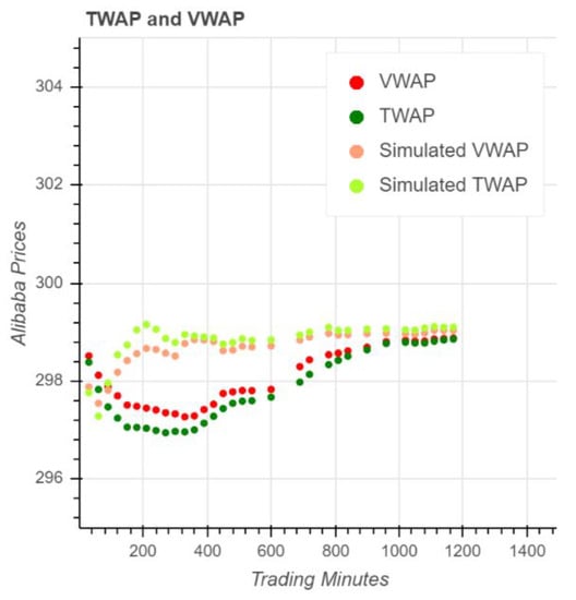 Figure 8. One of the implications can be backtesting execution algorithm parameters to optimize filling rates and portfolio positions. The left figure shows the simulated volume-weighted average price and time-weighted average price against original VWAP and TWAP. The spread gets narrow when trading continues until 1200 minutes. The prices are concentrated in a particular range, and WGAN-GP learns from the original prices and can even show the potential market uptrends.
8. Conclusions
The contributions can be summarized in the following:
- A complete WGAN-GP framework was proposed through extensive and systematic experiments for multiple asset classes, including stocks, futures, and cryptocurrency. Also, an in-depth analysis was given to fine-tune important hyperparameters. We trained our model on various datasets, including the Hong Kong Stock Market Hang Seng Index composite stocks, precious metal futures contracts listed on the Chicago Mercantile Exchange, the Japan Exchange Group, and cryptocurrency spots and perpetual contracts on Binance at various minute-level intervals. After generating 836,280 data points from 90,900 epochs, we showed that WGAN-GP can be trained as a probabilistic model with stability, scalability and robustness for price simulations.
- From an asset classes perspective, we find that 2269.HK has the largest MAE-R/Tick among Hang Seng Index stocks. Platinum assets like TPL (TOCOM Platinum on the Tokyo Commodity Exchange) and PLE (Platinum (Globex) NYMEX on the Chicago Mercantile Exchange) have relatively larger MAE-R/Tick than a gold asset like GCE and TGD. BTC, ETH, and BNB spots and perpetual futures have the largest MAE-R/Tick values. Many interesting topics remain to work on. First, we can further extend to other markets like The Standard and Poor’s 500, Nikkei 225, KOSPI 200 Index, CSI Small 500 Index, and the DAX Performance Index. Second, derivatives, especially non-linear products like option pricing, can be simulated against historical data.
- From a trading frequency perspective, WGAN-GP can be used to simulate possible price datasets at various minute-level intervals. We proposed to evaluate the outcomes by comparing the generated synthetic distribution against the original data distribution at multiple time intervals, including one, two, three, four, five, ten and fifteen minutes. When the model goes to the production environment, for execution considerations, some statistics for evaluation such as the quantity of executed orders, prediction of inter-arrival orders, cancellation rates and the best bid and best ask can be implemented.
To sum up, our results show that WGAN-GP can simulate asset prices and show a market simulator’s potential for trading analysis. We might be the first to look into multi-asset classes in a systematic approach with minute level intervals across stocks, futures and cryptocurrencies markets. We also contribute to quantitative analysis methodology for generated and original price data quality.
Author Contributions
Conceptualization, F.H. and J.Z.; methodology and visualization, F.H.; resources and curation, J.Z.; writing—original draft preparation, F.H.; writing—review and editing, X.M.; supervision, J.Z. and funding acquisition, J.Z. All authors have read and agreed to the published version of the manuscript.
Funding
This work was supported by Hong Kong Research Grant Council Grants 16208120 and Grants 16204718.
Institutional Review Board Statement
Not applicable.
Informed Consent Statement
Informed consent was obtained from all subjects involved in the study.
Data Availability Statement
Data that supports the findings of this study are available from the corresponding author upon reasonable request. Restrictions apply to the availability of data.
Acknowledgments
Thanks, SiuTim Wong, Luxu Liang for providing calculations support.
Conflicts of Interest
The authors declare no conflict of interest.
Abbreviations
The following abbreviations are used in this manuscript:
| TGD | TOCOM Gold on Tokyo Commodity Exchange |
| TPL | TOCOM Platinum on Tokyo Commodity Exchange |
| GCE | Gold (Globex) COMEX on Chicago Mercantile Exchange |
| PLE | Platinum (Globex) NYMEX on Chicago Mercantile Exchange |
| CME | COMEX on Chicago Mercantile Exchange |
| JPX | Japan Exchange Group |
| WGAN-GP | Wasserstein Generative Adversarial Networks-Gradient Penalty |
| HSI | Hang Seng Indexes |
Notes
| 1 | https://help.yahoo.com/kb/SLN2311.html/, accessed on 8 May 2021. |
| 2 | https://www.cryptodatadownload.com/data/binance/, accessed on 8 May 2021. |
References
- Abraham, Jethin, Daniel Higdon, John Nelson, and Juan Ibarra. 2018. Cryptocurrency price prediction using tweet volumes and sentiment analysis. SMU Data Science Review 1: 1. [Google Scholar]
- Ariyo, Adebiyi A., Adewumi O. Adewumi, and Charles K. Ayo. 2014. Stock price prediction using the ARIMA model. Paper presented at the 2014 UKSim-AMSS 16th International Conference on Computer Modelling and Simulation, Cambridge, UK, March 26–28; pp. 106–12. [Google Scholar]
- Arjovsky, Martin, Soumith Chintala, and Léon Bottou. 2017. Wasserstein generative adversarial networks. In International Conference on Machine Learning. Sydney: PMLR, pp. 214–23. [Google Scholar]
- Baur, Dirk G., and Lai T. Hoang. 2021. A crypto safe haven against Bitcoin. Finance Research Letters 38: 101431. [Google Scholar] [CrossRef]
- Binance. n.d. Available online: https://www.binance.com/en (accessed on 7 January 2022).
- CME Gold Futures and Options. n.d. Available online: https://www.cmegroup.com/markets/metals/precious/gold.html (accessed on 8 May 2021).
- CME Platinum Futures and Options. n.d. Available online: https://www.cmegroup.com/markets/metals/precious/platinum.html (accessed on 8 May 2021).
- Foster, Ernest Allen. 2002. Commodity Futures Price Prediction: An Artificial Intelligence Approach. Doctoral dissertation, University of Georgia, Athens, GA, USA. [Google Scholar]
- Goodfellow, Ian, Jean Pouget-Abadie, Mehdi Mirza, Bing Xu, David Warde-Farley, Sherjil Ozair, Aaron Courville, and Yoshua Bengio. 2014. Generative adversarial nets. Advances in Neural Information Processing Systems. 27. Available online: https://proceedings.neurips.cc/paper/2014/file/5ca3e9b122f61f8f06494c97b1afccf3-Paper.pdf (accessed on 8 May 2021).
- Gulrajani, Ishaan, Faruk Ahmed, Martin Arjovsky, Vincent Dumoulin, and Aaron Courville. 2017. Improved training of wasserstein gans. arXiv arXiv:1704.00028. [Google Scholar]
- Hong Kong Exchanges and Clearing Limited. n.d. Available online: https://www.hkex.com.hk/ (accessed on 8 May 2021).
- JPX Gold Futures and Options. n.d. Available online: https://www.jpx.co.jp/english/derivatives/products/precious-metals/gold-standard-futures/index.html (accessed on 8 May 2021).
- JPX Platinum Futures and Options. n.d. Available online: https://www.jpx.co.jp/english/derivatives/products/precious-metals/platinum-standard-futures/01.html (accessed on 8 May 2021).
- Kakushadze, Zura. 2016. 101 formulaic alphas. Wilmott 84: 72–81. [Google Scholar] [CrossRef]
- Kang, Sang Hoon, Ron McIver, and Seong-Min Yoon. 2017. Dynamic spillover effects among crude oil, precious metal, and agricultural commodity futures markets. Energy Economics 62: 19–32. [Google Scholar] [CrossRef]
- Kim, Harold Y., and Jianping P. Mei. 2001. What makes the stock market jump? An analysis of political risk on Hong Kong stock returns. Journal of International Money and Finance 20: 1003–16. [Google Scholar] [CrossRef]
- Kyriazis, Nikolaos A., Kalliopi Daskalou, Marios Arampatzis, Paraskevi Prassa, and Evangelia Papaioannou. 2019. Estimating the volatility of cryptocurrencies during bearish markets by employing GARCH models. Heliyon 5: e02239. [Google Scholar] [CrossRef] [PubMed]
- Lee, Seungho, Nabil El Meslmani, and Lorne N. Switzer. 2020. Pricing efficiency and arbitrage in the bitcoin spot and futures markets. Research in International Business and Finance 53: 101200. [Google Scholar] [CrossRef]
- Lezmi, Edmond, Jules Roche, Thierry Roncalli, and Jiali Xu. 2020. Improving the Robustness of Trading Strategy Backtesting with Boltzmann Machines and Generative Adversarial Networks. Available online: https://papers.ssrn.com/sol3/papers.cfm?abstract_id=3645473 (accessed on 8 May 2021).
- Li, Junyi, Xintong Wang, Yaoyang Lin, Arunesh Sinha, and Michael Wellman. 2020. Generating realistic stock market order streams. Paper presented at the AAAI Conference on Artificial Intelligence, Taipei, Taiwan, April 11–13; vol. 34, pp. 727–34. [Google Scholar]
- Mensi, Walid, Jose Arroeola Hernandez, Seong-Min Yoon, Xuan Vinh Vo, and Sang Hoon Kang. 2021. Spillovers and connectedness between major precious metals and major currency markets: The role of frequency factor. International Review of Financial Analysis 74: 101672. [Google Scholar] [CrossRef]
- Meyer, David R., and George Guernsey. 2017. Hong Kong and Singapore exchanges confront high frequency trading. Asia Pacific Business Review 23: 63–89. [Google Scholar] [CrossRef]
- Palamalai, Srinivasan, K. Krishna Kumar, and Bipasha Maity. 2021. Testing the random walk hypothesis for leading cryptocurrencies. Borsa Istanbul Review 21: 256–68. [Google Scholar] [CrossRef]
- Rosolia, Antonio, and Joerg Osterrieder. 2021. Analyzing Deep Generated Financial Time Series for Various Asset Classes. Available online: https://papers.ssrn.com/sol3/papers.cfm?abstract_id=3898792 (accessed on 8 May 2021).
- Samuel, Rikli, Bigler Daniel Nico, Pfenninger Moritz, and Osterrieder Joerg. 2021. Wasserstein GAN: Deep Generation applied on Bitcoins financial time series. arXiv arXiv:2107.06008. [Google Scholar]
- Smith, Leslie N. 2017. Cyclical learning rates for training neural networks. Paper presented at the 2017 IEEE Winter Conference on Applications of Computer Vision (WACV), Santa Rosa, CA, USA, March 24–31; pp. 464–72. [Google Scholar]
- Xu, Ke, Xinwei Zheng, Deng Pan, Li Xing, and Xuekui Zhang. 2020. Stock Market Openness and Market Quality: Evidence from the Shanghai–Hong Kong Stock Connect Program. Journal of Financial Research 43: 373–406. [Google Scholar] [CrossRef]
- Xu, Xiaoqing Eleanor, and Hung-Gay Fung. 2005. Cross-market linkages between US and Japanese precious metals futures trading. Journal of International Financial Markets, Institutions and Money 15: 107–24. [Google Scholar] [CrossRef]
- Yahoo Finance. n.d. Available online: https://help.yahoo.com/kb/SLN2311.html (accessed on 7 January 2022).
Publisher’s Note: MDPI stays neutral with regard to jurisdictional claims in published maps and institutional affiliations. |
© 2022 by the authors. Licensee MDPI, Basel, Switzerland. This article is an open access article distributed under the terms and conditions of the Creative Commons Attribution (CC BY) license (https://creativecommons.org/licenses/by/4.0/).