Autoencoder-Based Three-Factor Model for the Yield Curve of Japanese Government Bonds and a Trading Strategy

Abstract

Interest rates are representative indicators that reflect the degree of economic activity. The yield curve, which combines government bond interest rates by maturity, fluctuates to reflect various macroeconomic factors. Central bank monetary policy is one of the significant factors influencing interest rate markets. Generally, when the economy slows down, the central bank tries to stimulate the economy by lowering the policy rate to establish an environment in which companies and individuals can easily raise funds. In Japan, the shape of the yield curve has changed significantly in recent years following major changes in monetary policy. Therefore, an increasing need exists for a model that can flexibly respond to the various shapes of yield curves. In this research, we construct a three-factor model to represent the Japanese yield curve using the machine learning approach of an autoencoder. In addition, we focus on the model parameters of the intermediate layer of the neural network that constitute the autoencoder and confirm that the three automatically generated factors represent the “Level,” “Curvature,” and “Slope” of the yield curve. Furthermore, we develop a long–short strategy for Japanese government bonds by setting their valuation with the autoencoder, and we confirm good performance compared with the trend-follow investment strategy.

1. Introduction

The interest rate on government bond yields is a representative indicator of macroeconomic fundamentals. Generally, when an economy is active, household consumption and corporate capital investment are also active. In such situations, the demands for raising funds increase even though the interest rate level is high. As a result, these demands lead to a further rise in interest rates on loans, corporate bonds, and government bonds. In addition, the interest rates of government and corporate bonds are affected by the credit risk of the issuer country or company. For example, when concern increases regarding the issuer’s financial and fiscal situations, the pressure on interest rates also increases due to the rise in fund procurement costs. Meanwhile, nominal interest rates are also affected by inflation. For instance, the relationship that the nominal interest rate rises when peoples’ inflation expectations rise is known as the Fisher equation. Thus, while incorporating changes in various macroeconomic environments, the market price of government bonds and the interest rates also change. In addition to the macroeconomic environment of the market’s home country, various factors in foreign markets are transmitted to the domestic interest rate market through interest rate arbitrage transactions.

Another factor significantly impacting the interest rate market is the monetary policy of the central bank. Traditionally, central banks adjust the level of short-term interest rates as the policy rate. For example, when the economy slows down, the central bank tries to stimulate the economy by lowering the policy rate to establish an environment in which companies and individuals can easily raise funds. Conversely, when the economy is overheating, the central bank will leverage the opposite mechanism by raising the policy rate. For these purposes, the central bank generally implements monetary policy by inducing short-term interest rates through open market operations.

However, in 2016, the Bank of Japan (BOJ) introduced the “Quantitative and Qualitative Monetary Easing with Yield Curve Control” that sets the target for long-term and short-term interest rates (Bank of Japan 2016). The “yield curve” is formed by the interest rates of government bonds by maturities, with movements that reflect the interest rate fluctuation factors described above. The BOJ’s yield curve control policy significantly affects the fluctuation characteristics of the yield curve because it sets a guidance target for long-term and short-term interest rates. Under such monetary policy, the medium-term and short-term interest rates of Japanese government bonds are currently negative. We show the change of the Japanese yield curve in Figure 1. In the past, the yield curve fluctuated in the positive area, but recently, it has become negative in not only the short-term but also the long-term interest rates. Furthermore, the short- and medium-term interest rates’ curve has become almost flat in the negative area. In addition, the volatility of the short-term to long-term interest rates has declined. So, there is now an increasing need for a yield curve model that can flexibly cope with these types of changing yield curve shapes.

Analysis of the yield curve shape is important for forecasting fluctuations for trading purposes and risk management for bondholders to understand the characteristics of the market environment. With these backgrounds, this research focuses on the Japanese interest rate market. We propose a model that flexibly describes the shape of the yield curve and serves as a reference for evaluating the asset price of government bonds relative to the market environment.

Specifically, we develop a three-factor model that represents the yield curve of the Japanese government bond market using an autoencoder, a type of machine learning method structured as an artificial neural network. To propose such a method, we first design a simple self-encoder model with one hidden layer. By considering the model parameters of the neural network, we confirm that the three automatically generated factors represent the “Level,” “Curvature,” and “Slope” of the yield curve.

Various studies using complex neural network models exist today for financial market analysis and forecasting. For example, using neural network models, Krauss et al. (2017), analyzed the US stock market, Suimon (2018), forecasted the Japanese bond market, and Matthew et al. (2017), focused on commodity and foreign exchange markets. However, when a complex neural network model, such as deep learning, was used, risk management problems resulted in making interpretations of these models’ output results difficult. In financial businesses, accountability arises in many situations when forming investment strategy decisions and valuing assets held. Therefore, this research proposes a method that contributes to the transparency of decision making by constructing an interpretable yield curve model. Furthermore, we propose a method of using the autoencoder as a discriminator for overvalued and undervalued government bonds, and verify the prediction accuracy when using these in investment strategies.

2. Literature Review

In this research, we propose a factor model for the JGB yield curve using an autoencoder to develop a trading strategy for judging the overvaluation or undervaluation of each maturities’ government bonds. As a previous related study, with respect to yield curve modeling, there are some methods to estimate the yield curve from the government bonds’ market prices. According to Kikuchi and Shintani (2012), these methods are classified the following four types: (1) the piecewise polynomial method (McCulloch 1971, 1975), (Steeley 1991), the models of which use piecewise polynomials to express the discount function; (2) the non-parametric method (Tanggaard 1997), which does not assume any specific structure for the discount function; (3) the polynomial method (Schaefer 1981), which models the discount function with polynomials; and (4) the parsimonious function method (Nelson and Siegel 1987), (Svensson 1995), which assumes specific functional forms for the yield curve term structure.

Regarding the forecasting model of yield curve, Diebold and Li (2006), simulated the US yield curve by using the Nelson–Siegel model (Nelson and Siegel 1987) and predicted the additional changes of the model’s three factors by using the AR (Autoregressive) model. In addition, the authors in Diebold et al. (2006), analyzed the relationship between the Nelson–Siegel factors and macroeconomic variables. They demonstrated that the level factor is related to inflation, and the slope factor is related to economic activity. However, the curvature factor did not have a clear relationship with macroeconomic variables.

The research of Reisman and Zohar (2004), extracted three principal component factors with PCA, simulated the time series of each factor, and predicted the yield curve changes based on the time series model factors. In addition, Moench (2008), and Ludvigson and Ng (2009), conducted PCA on multiple macro indexes and predicted the interest rates based on the established macro-based PCA factors.

Furthermore, Suimon (2018), also proposed a yield curve model based on machine learning methods, and expressed the interest rate term structure by focusing on the relative relationship of the three periods (5-, 10-, and 20-year interest rates) of the yield curve instead of the three Nelson–Siegel factors. Then, using Long Short-Term Memory (LSTM), they forecasted the long-term interest rate. Extending this research, Suimon et al. (2019a, 2019b), incorporated Japanese and US interest rate information directly into a neural network model. Moreover, based on interest rate parity theory, Suimon et al. (2019c), incorporated the Dollar–Yen exchange rate in addition to the US and Japanese interest rates into a neural network model.

Machine learning methods for modeling financial markets have been developed, particularly in the forecasting of stock markets. For example, multiple investigations on stock price prediction with neural networks have been reported (Soni 2011). Olson and Mossman (2003), demonstrated the utility of a neural network model for the Canadian stock market forecasting with multiple accounting ratios as the input data. Research by Krauss et al. (2017), predicted next-day US stock market pricing by combining three machine learning methods of deep neural networks, gradient-boosted trees, and random forests. They reported the prediction accuracy of this combined method exceeded the individual method’s prediction accuracies. In another recent study on forecasting stock returns in the cross-section, Abe and Nakayama (2018), showed that deep neural networks outperform shallow neural networks as well as other typical machine learning models. Another deep learning-based research of financial markets apart from the stock market was performed by Matthew et al. (2017), who focused on commodity and foreign exchange markets.

3. Term Structure Model of The Yield Curve

3.1. Changes in Government Bond Interest Rates

Interest rates (yields of government bonds) are representative indicators of the macroeconomic environment. When economic activity is booming, interest rates on bank loans, corporate bonds, and government bonds experience upward pressure due to the growing demand for various funds. In addition, interest rates on government bonds and corporate bonds are affected by the credit risk of the issuing country or company. Interest rate fluctuation factors in overseas markets also affect the domestic market through financial arbitrage transactions. Through these interactions, the market price of the government bonds is formed while incorporating changes in the market environment, and the interest rates calculated from government bond prices change.

3.2. Term Structure Model of The Japanese Government Bond Yield Curve

Figure 2 plots a history of several interest rates with varying maturities. Currently in Japan, in addition to short-term discounted government bonds, government bonds with maturities of 2, 5, 10, 20, 30, and 40 years are issued, and there are market interest rates on government bonds with a range of maturities (Ministry of Finance 2019). The “Yield curve” shown in Figure 3 combines the interest rates of these maturities.

The shape of the yield curve can be expressed using a term structure model for interest rates. For example, using the Nelson–Siegel model (Nelson and Siegel 1987), the term structure of interest rates can be expressed by the following functional form. Here, y is the interest rate, τ is the term, and λ is a constant. The Nelson–Siegel model curve is fitted in Figure 3 to the actual Japanese government bond (JGB) yield curve according to

$$y\left(\tau \right)=F_1+F_2\left(\frac{1-e^{-\lambda \tau }}{\lambda \tau }\right)+F_3\left(\frac{1-e^{-\lambda \tau }}{\lambda \tau }-e^{-\lambda \tau }\right)$$

(1)

This model function consists of three factors of F, representing the level, slope, and curvature of the yield curve. The coefficients for each factor by maturities are shown in Figure 4. The Nelson–Siegel model is one in which a simple function approximately represents the shape of the yield curve. So, while it is convenient, it is also subject to restrictions on the shape of the model function.

Principal factors can also be extracted by performing principal component analysis (PCA) directly on interest rate data. Applied to weekly Japanese government bond yield data for 2, 5, 7, 10, 15, and 20 years after 1992, the results show nearly a 99% cumulative contribution of the third PCA factor. This suggests that the shape of the yield curve can be almost expressed. Figure 5 plots the shape of the eigenvector for each PCA factor showing that the first, second, and third factors represent the level, slope, and curvature of the yield curve, respectively.

4. Autoencoder-Based Model Design for the Yield Curve

4.1. Autoencoder

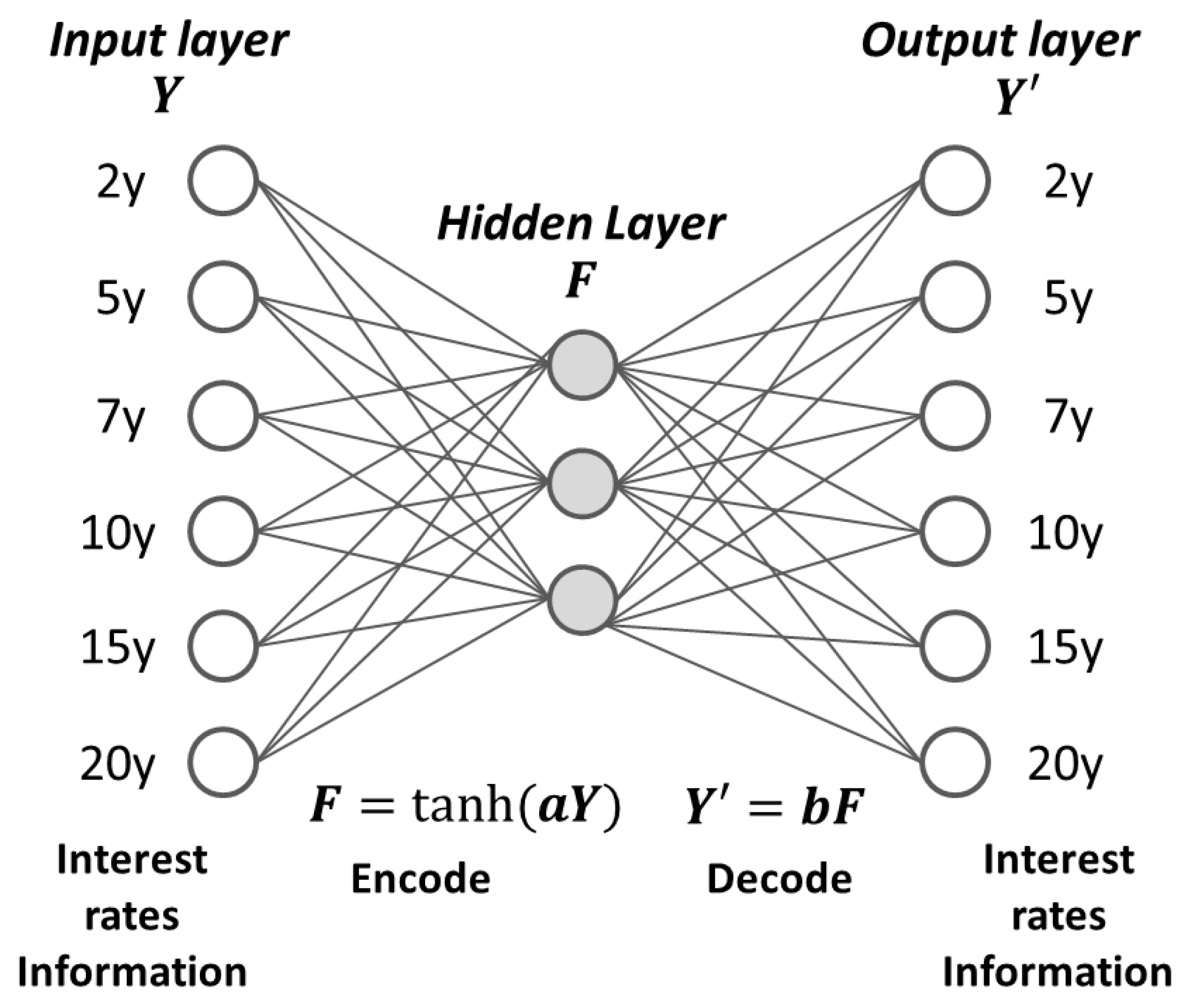
We next construct a model that expresses the yield curve of the Japanese government bond market using an autoencoder, an algorithm for dimension compression using neural networks (Hinton and Salakhutdinov 2006). Principal component analysis is an example of a linear dimension compression. With autoencoders, the same training data is learned through the input and output layers of a neural network. By increasing the number of nodes in a hidden layer, more complex yield curve shapes can be expressed. In this research, we construct neural network models with 2, 3, and 4 nodes in the hidden layer for comparison.

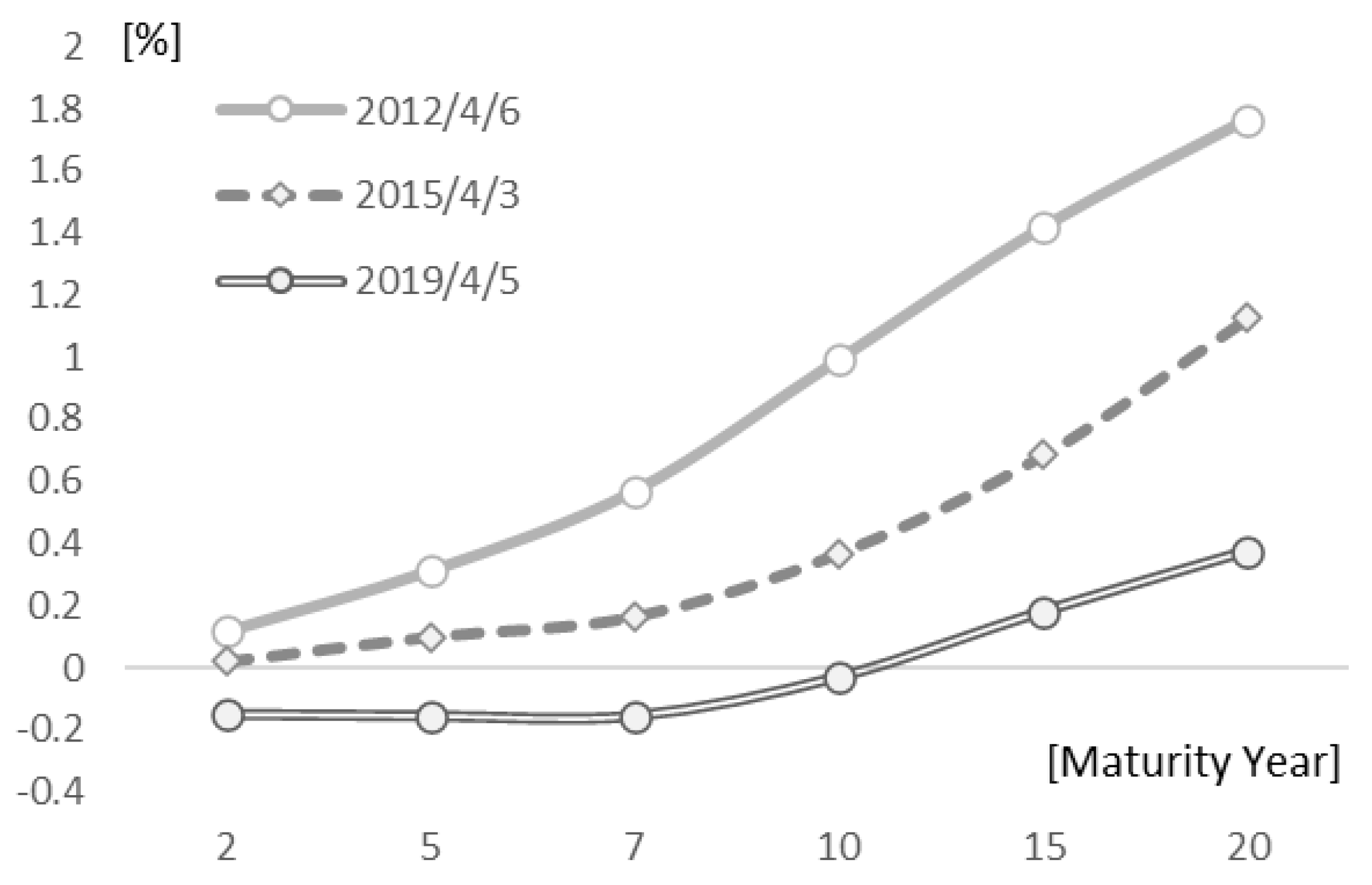
Figure 6 illustrates how we incorporate 2-, 5-, 7-, 10-, 15-, and 20-year interest rate data into a learning model. In this autoencoder model, Y is the vector of the input information, 2-, 5-, 7-, 10-, 15-, and 20-year interest rate data and the activation function to the hidden layer is hyperbolic tangent. The output information of the model is Y′. We estimate the model parameters b and a so that the input information Y and the output information Y′ matches. we use weekly data from July 1992 to July 2019 to estimate the model. We interpret each node of the hidden layer in the self-encoder by assigning a linear function to represent the path to the output layer and consider the function’s coefficient.

$${\mathit{Y}}^{\mathbf{\prime }}=\mathit{b}\mathit{F}=b\left[\tanh \left(\mathit{a}\mathit{Y}\right)\right]$$

(2)

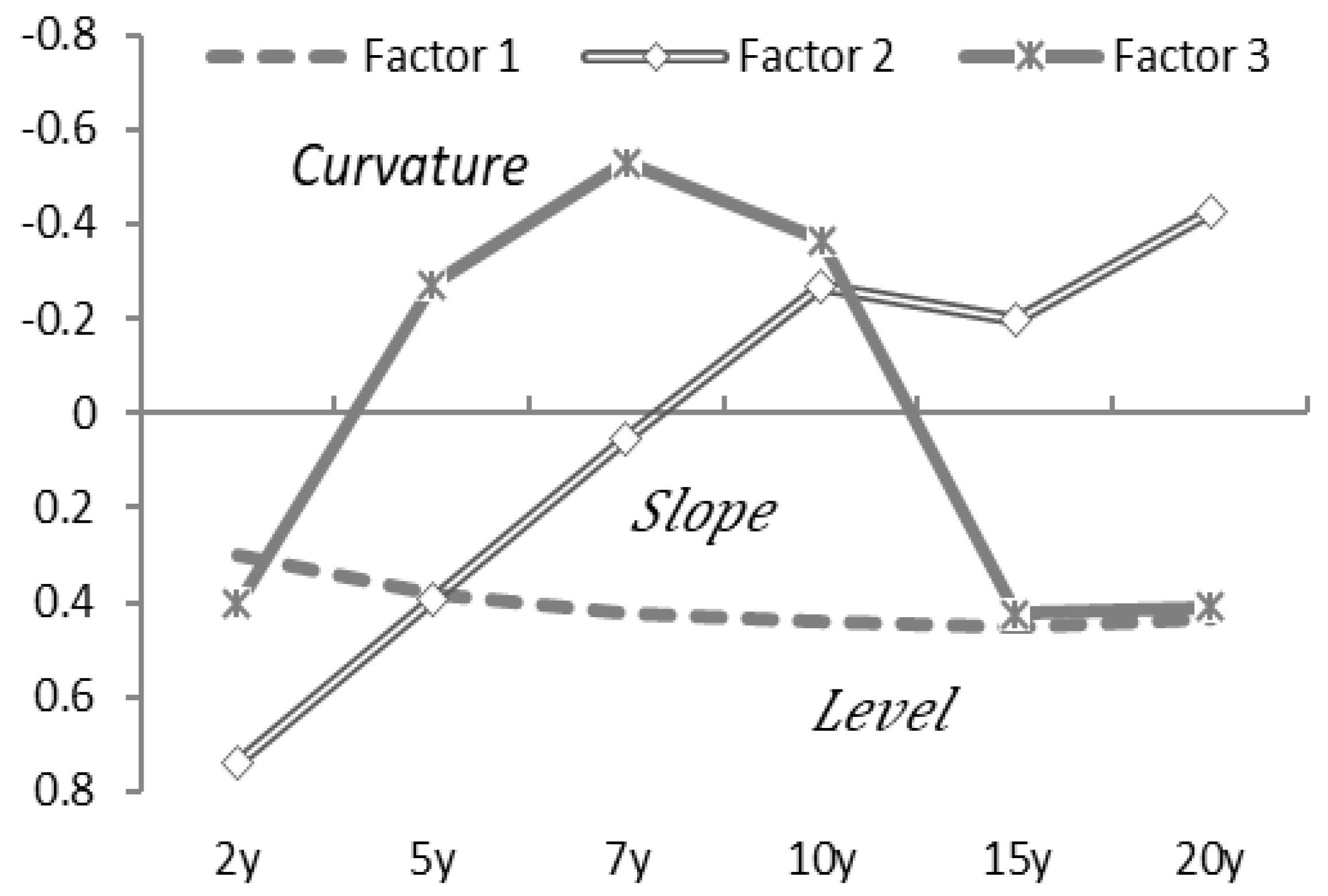
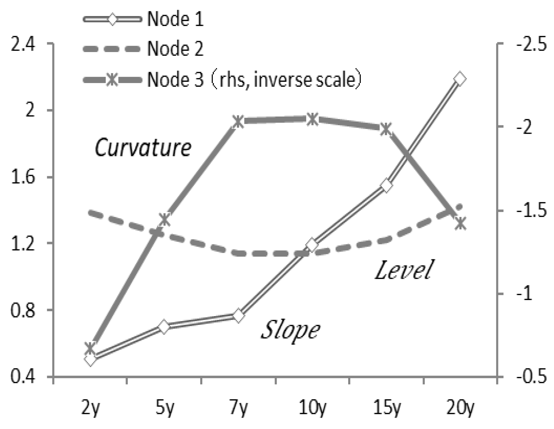
First, we analyze the model with a hidden layer comprised of three nodes. Figure 7 shows the coefficient b of the linear function representing the output from the hidden layer, which provides the correspondence between the hidden layer’s nodes and the output layer’s nodes. Each node in the hidden layer can be interpreted as the level, slope, and curvature of the yield curve.

Based on these results, Figure 8 compares the value of each node with the actual interest rate level and interest rate spread (i.e., the interest rate difference). For example, comparing Node 2, representing a level, with a two-year interest rate near the start of the yield curve, the two are approximately linked. Comparing Node 1, interpreted as the slope, with the 2–20-year interest rate spread (i.e., 20-year yield - 2-year yield), both move similarly. Node 3, interpreted as the curvature of the yield curve centered on long-term interest rates, compared with the 2-10-20 year butterfly spread (i.e., 2 × 10-year yield - 10-year yield - 20-year yield), also moves similarly in Figure 8.

Next, we review the results with only two nodes in the hidden layer. Figure 9 plots the coefficients of the linear function representing the hidden layer for each node to the output layer. With only two hidden layers, the nodes are interpreted as the curvature of the yield curve and the combined slope and level of the yield curve.

Figure 10 plots comparisons between the value of each node in the hidden layer with the actual interest rate spread. Node 1, interpreted as the slope, moves similarly to the 2-20-year interest rate spread (i.e., 20-year yield - 2-year yield). Node 2, interpreted as a curvature of the yield curve centered on the long-term interest rate, is approximately linked to the 2-7-20 year butterfly spread (i.e., 2 × 10-year yield - 7-year yield - 20-year yield).

Finally, we analyze the model with four nodes in the hidden layer. According to the coefficients of the linear function representing the output from the hidden layer, as shown in Figure 11, Node 1 represents the level, Node 3 represents the curvature, and Node 2 and Node 4 represent the slope. However, according to the shape of each coefficient vector, Node 1, Node 2, and Node 4 also include a curvature element. So, with four nodes in the hidden layer, the interpretation of each is not as straightforward as the models with two or three nodes. In the principal component analysis (PCA) described in Section 3, the cumulative contribution to the shape of the yield curve when using the third principal component factor was about 99%. So, as suggested by these results, the autoencoder can best represent the shape of the yield curve with three nodes in the hidden layer.

In this research, we proposed a yield curve model using an autoencoder. Like the Nelson–Siegel model (Nelson and Siegel 1987), and other known factor models (Svensson 1995) (Dai and Singleton 2000), the proposed model can express the shape of the yield curve by combining the three factors, curvature, level, and slope. The factor models, such as the Nelson–Siegel model and the Svensson model etc., that we mention above need to explicitly set a function form that expresses the shapes of the yield curve. However, the autoencoder-based model or neural network-based model have high flexibility for the expression of the yield curve because these models can set the function forms flexibly. With significant changes in monetary policy and other factors, the fluctuation characteristics of the yield curve also change, so a flexible functional form is required for the yield curve modeling. When using autoencoder-based model or neural network-based model, not only the model parameters but also hyperparameters and the number of nodes can be changed to increase the flexibility of the model function that express the shape of the yield curve.

Furthermore, when using PCA for the yield curve modeling and specifying the number of principal component factors, we cannot cover the contribution of the other PCA factors. However, when using an autoencoder for the modeling, all input information can be used via the network model. These points are advantages of the autoencoder-based model as a yield curve factor model compared to other factor models.

4.2. Autoencoder-Based Yield Curve Model and Trading Strategy

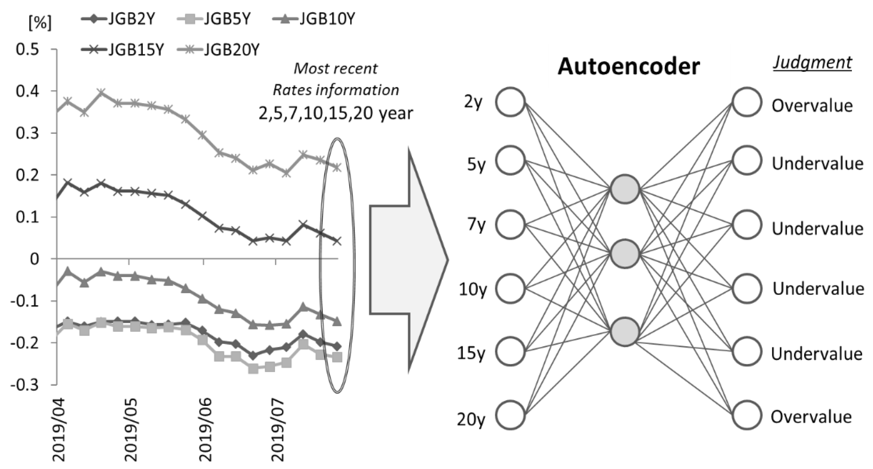
From the viewpoint of asset price evaluation and investment strategies for government bonds, we propose using an autoencoder that models the shape of the yield curve. The interest rate output by the trained autoencoder is calculated based on the relative relationship with the interest rates of the other maturities. So, in this section, we apply the trained autoencoder as a discriminator for overvalued or undervalued government bonds compared to other maturities. We also construct a long–short strategy for government bonds based on these overvalued and undervalued evaluations to verify its performance.

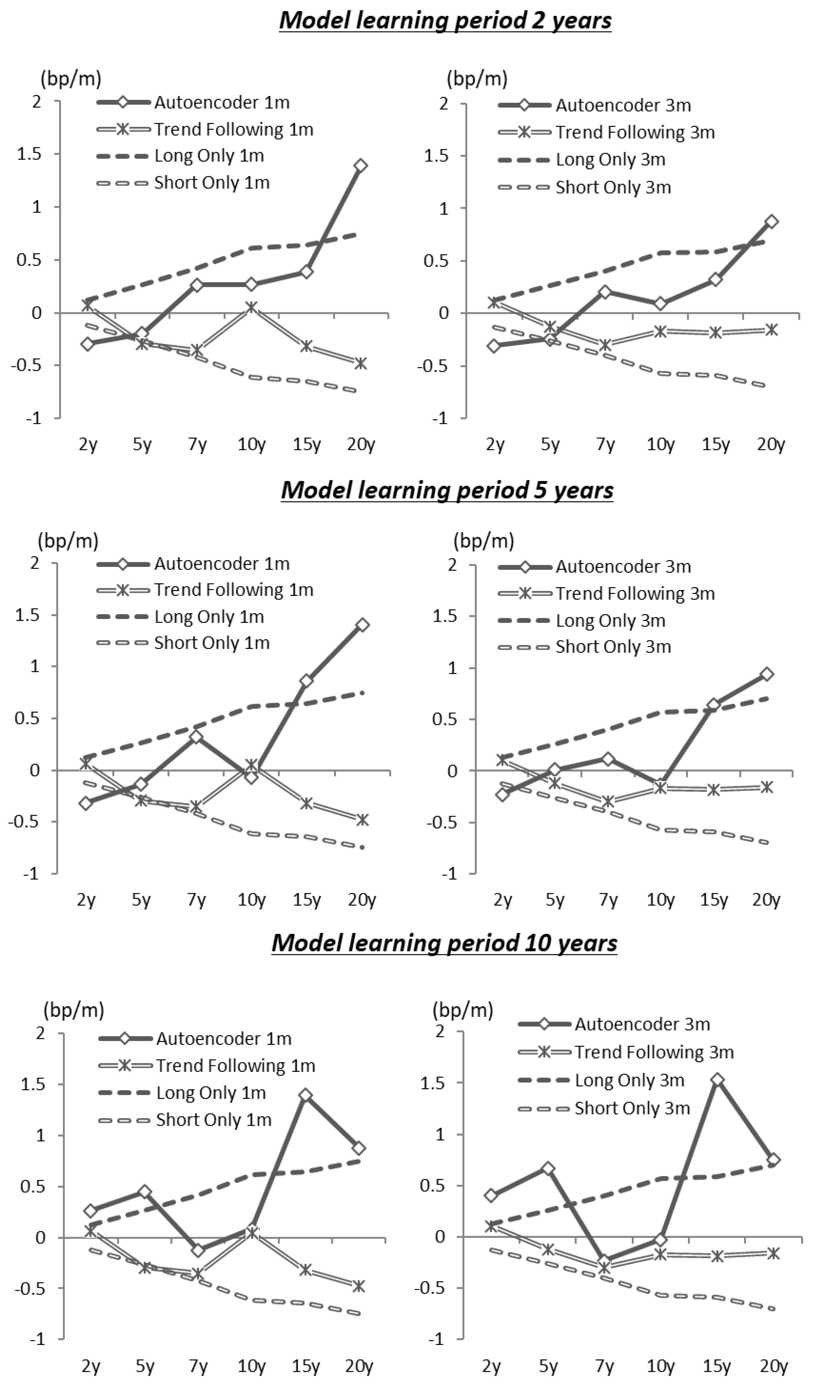
The interest rate data for each maturity at the time of investment is input to the learned autoencoder, and we define the output interest rate as the reference interest rate. For each maturity, if the interest rate at the time of investment is higher than the reference interest rate, we judge the government bond as undervalued as shown in Figure 12, so we long (buy) the bond. On the other hand, if the interest rate is lower than the base interest rate, we short (sell) the bond. The investment period for each position is one or three months. For training the autoencoder, we include data from the previous 2, 5, and 10 years, excluding data at the time of the model update, and update the models annually. Weekly interest rate data from July 1992 to July 2019 is used for the investment simulation.

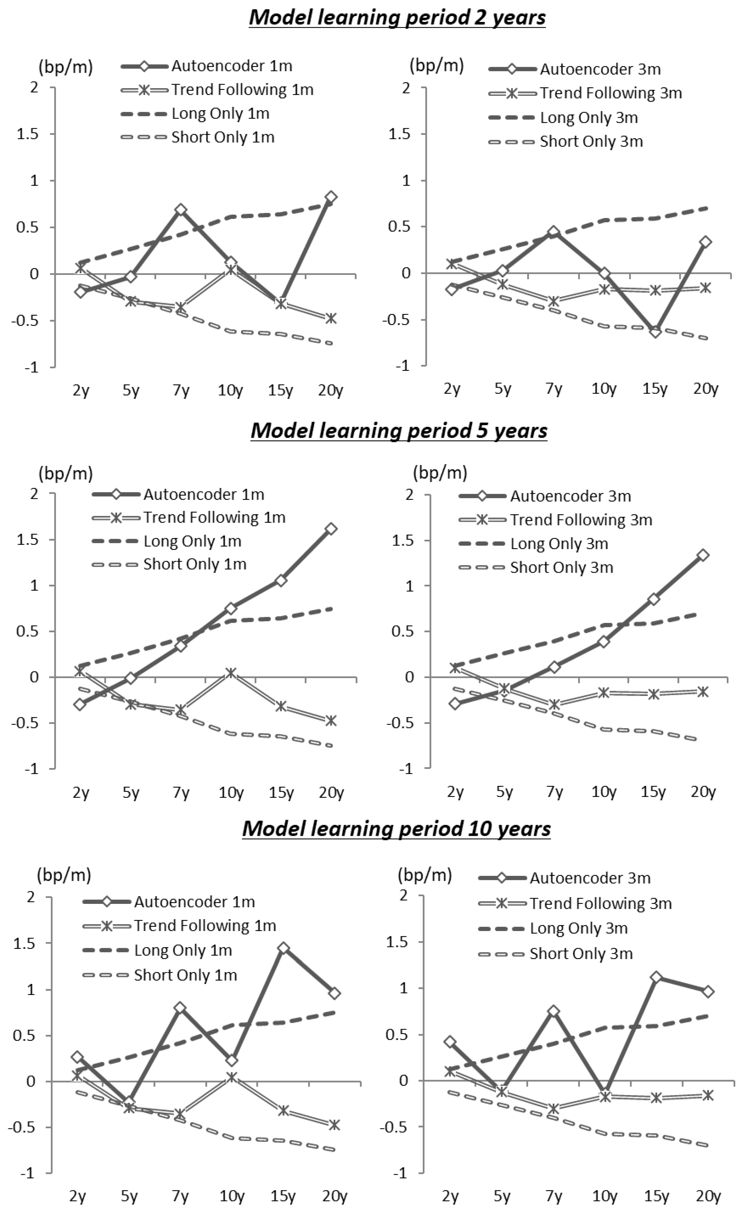
Figure 13 shows the simulation results for the autoencoder with three hidden layer nodes modeling the average capital gain over one month for each long–short strategy. The unit of the capital gain is bp (0.01%). For the long position, the decrease in interest rates during the investment period is the capital gain, and, for the short position, the increase in interest rates is the capital gain. To verify the accuracy of the interest rate forecasting by the model, we do not consider the effects of carry and rolldown and repo cost when making a short position. For the comparison of this trading strategy, we present the results of a trend-follow investment strategy (i.e., long if the interest rate declines from the previous week at each investment period, and short if interest rates rise) along with the results of investment strategies that are always a long (short) position.

The performance of the investment simulation depends on the number of nodes in the hidden layer, the learning period of the model, and the maturity of the government bonds to be invested. Figure 13 shows the result of the proposed strategy with the three-node model with a learning period of about 5 years and an investment period of 1 month. For the 10-year and 20-year government bonds’ investment strategies, these results suggest that the proposed model has a higher investment return than the trend-follow investment strategy.

The results from the models with two or four nodes in the hidden layer are included in Appendix A. For both cases, the performances are similar to the model with three hidden layer nodes. However, for the one-month investment strategy of 10-year and 20-year government bonds using 5 years for the learning period, the performance of the three-node case is better.

In this strategy, the trained autoencoder calculates the base interest rate from the relationships with the other maturities’ interest rates. If the interest rate of the target maturity is distorted compared to the other rates, there is merit in that the autoencoder’s judgment can automatically construct the investment position for correcting the distortion. However, such interest rate distortions between maturities are corrected in a relatively short period, so the one-month investment period is better than three months, as shown in these results of the investment performance.

The performance of the model is good when the learning period is approximately 5 years, which is likely due to the frequency of monetary policy changes that significantly affect the characteristics of the interest rate market. Based on the Yu-cho Foundation (2018), Figure 14 shows the timing of recent major Japanese monetary policy changes and illustrates that the monetary policy framework changes every two to five years. Considering this frequency of change, if the model learning period is 10 years, it is difficult to respond to these changes in the market characteristics. On the other hand, if the model learning period is 2 years, the number of data samples for learning is too small in the form of weekly granular data. From these observations, a learning period of 5 years is presumed to offer the best performance.

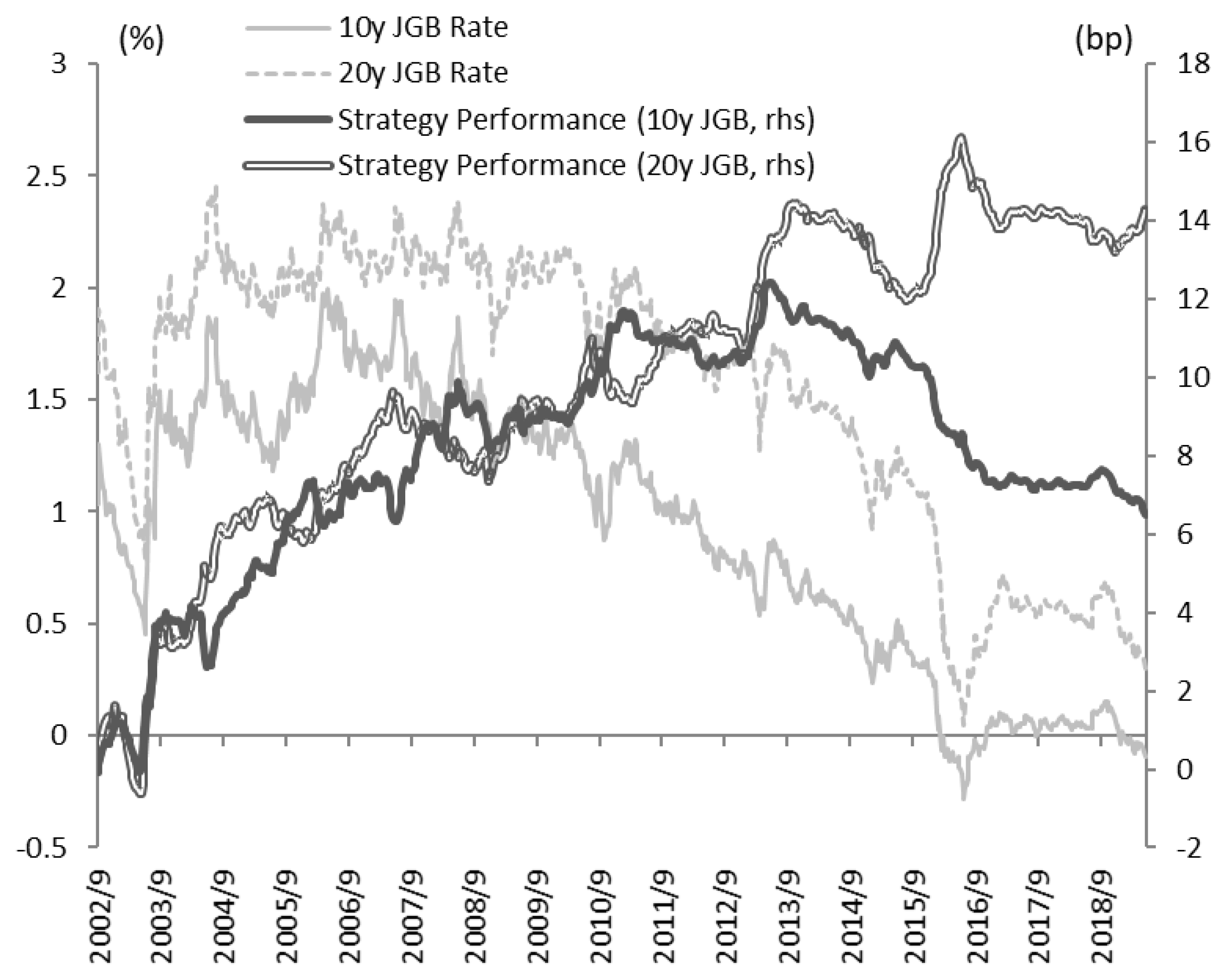
In summary, we confirmed the relative effectiveness of the performance of the 10-year and 20-year government bonds strategies with a learning period of 5 years and an investment period of 1 month. Figure 15 shows the cumulative performance of this strategy that verifies the positive cumulative returns for both strategies. However, in the 10-year government bonds strategy, the cumulative returns decline significantly after the beginning of 2016. Figure 15 also includes the 10-year and 20-year bond yields, showing that the 10-year bond yield fell nearly to 0% since the introduction of the “Quantitative and Qualitative Monetary Easing with a Negative Interest Rate” policy in January 2016. Furthermore, after the introduction of the “Quantitative and Qualitative Monetary Easing with Yield Curve Control” policy in September 2016, the 10-year bond yield remains strictly around 0%. Therefore, we see that such rigidity in market interest rates can cause the sluggish performance of the long–short strategies for 10-year government bonds.

4.3. Comparison with Other Strategy Models

In the previous section, we confirmed the performance of the investment strategies that use the autoencoder as a discriminator to judge overvaluation or undervaluation for each maturities’ government bonds. In this strategy, as shown in Figure 16, the investment decision is based on the interest rate data at the time of the investment, without directly using the historical data before the investment day. Nevertheless, a relatively stable return is obtained.

On the other hand, this investment strategy is ancillary as it was devised during the development of the autoencoder for the yield curve factor model. Typically, when making an investment strategy for government bonds, the historical data of the interest rates would be incorporated. For example, Suimon (2018), and Suimon et al. (2019b), proposed an investment strategy based on a neural network model that learned with historical time series data of interest rates. These studies demonstrated the usefulness of an LSTM (Long Short-Term Memory) (Hochreiter and Schmidhuber 1997) model that also learned to make predictions based on interest rate time series data. In addition, VAR (Vector autoregression)-based strategies (Estrella and Mishkin 1997; Ang and Piazzesi 2003; Afonso and Martins 2012) are also known as investment strategies for the government bonds market by using the historical interest rates data. Based on these past studies, we next implement an investment strategy using the LSTM and VAR model trained on interest rate historical data to compare its investment performance with that of the autoencoder model.

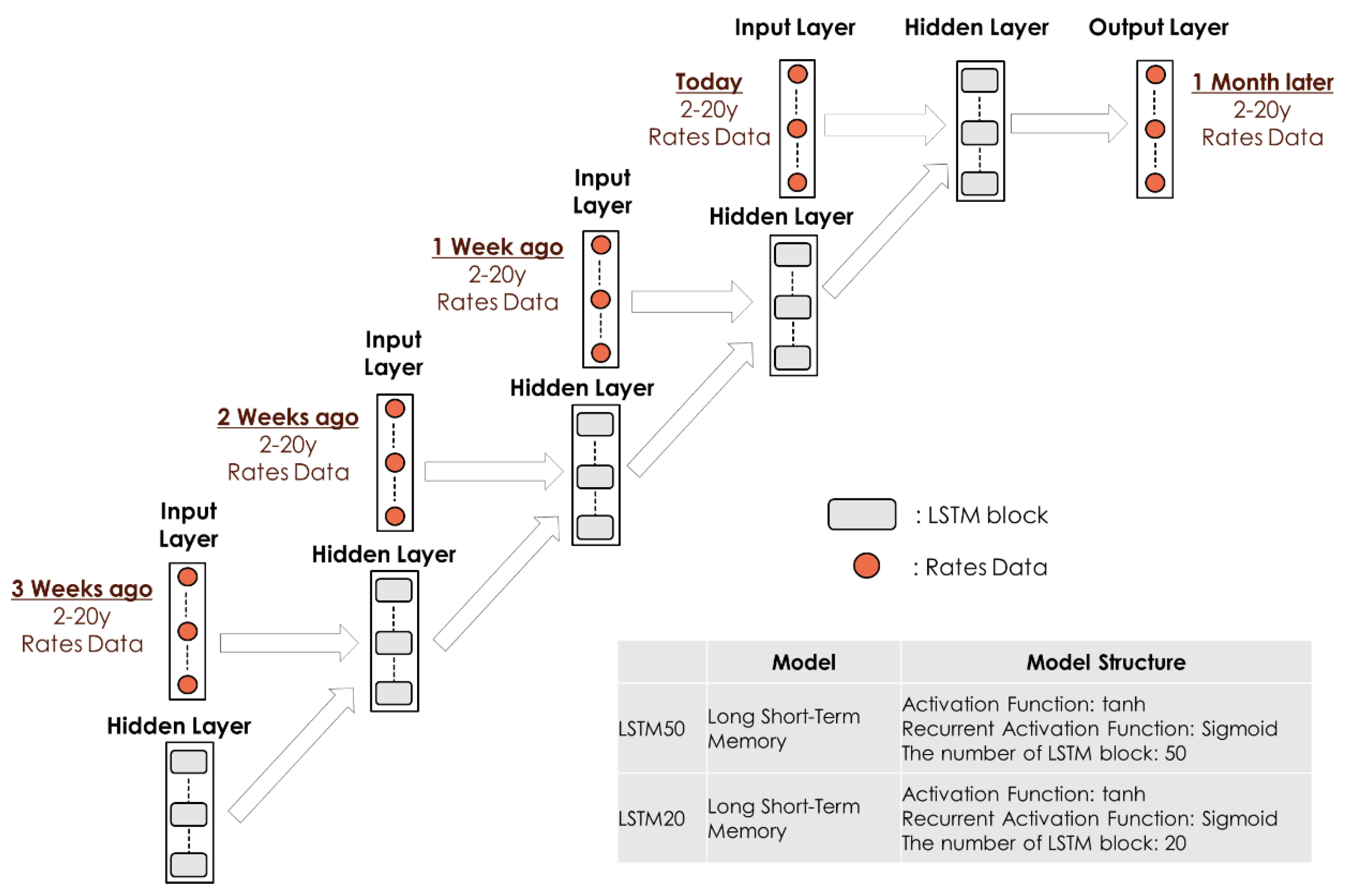
The LSTM model is a type of Recurrent Neural Network (RNN) model that inputs past time series information sequentially. Figure 17 illustrates the relationship between the input and output information of the interest rate data for the LSTM model we implement here. The structure of the LSTM block in Figure 17 is as shown in Figure 18. As shown in Figure 16, in addition to the interest rate data at the time of investment, the interest rate data of the previous weeks are used as input information for the model. Then, the LSTM model learns the correspondence between these past interest rates and future interest rates.

Furthermore, as with LSTM, we implement a VAR model which use the interest rate information of the past few weeks as the input information and which use the interest rate information of one month ahead as the output information. Here, let ${\mathit{y}}_{\mathit{t}}$ be the interest rate of one month ahead and ${\mathit{y}}_{\mathit{t}-\mathit{i}}$ be the weekly interest rate of the past three weeks including the time of investment. ${\Phi }_i$ and $\mathit{C}$ are the model parameters.

$${\mathit{y}}_{\mathit{t}}={\Phi }_1{\mathit{y}}_{\mathit{t}\mathbf{-}\mathbf{1}}+{\Phi }_2{\mathit{y}}_{\mathit{t}\mathbf{-}\mathbf{2}}+{\Phi }_3{\mathit{y}}_{\mathit{t}\mathbf{-}\mathbf{3}}+{\Phi }_4{\mathit{y}}_{\mathit{t}\mathbf{-}\mathbf{4}}+\mathit{C}+{\mathit{\epsilon }}_{\mathit{t}}$$

(3)

Using the LSTM model and VAR model, we predict the interest rate one month later and decide to buy or sell the government bonds for each maturity based on the relationship between the actual interest rate at the time of investment and the forecasted future interest rate. For example, if the predicted interest rate one month ahead according to the model is higher than the interest rate at the time of investment, we expect the interest rate will rise, so we short (sell) the government bond. On the other hand, if the predicted interest rate is lower than the current interest rate, we expect the interest rate will fall, and we long (buy) the government bond.

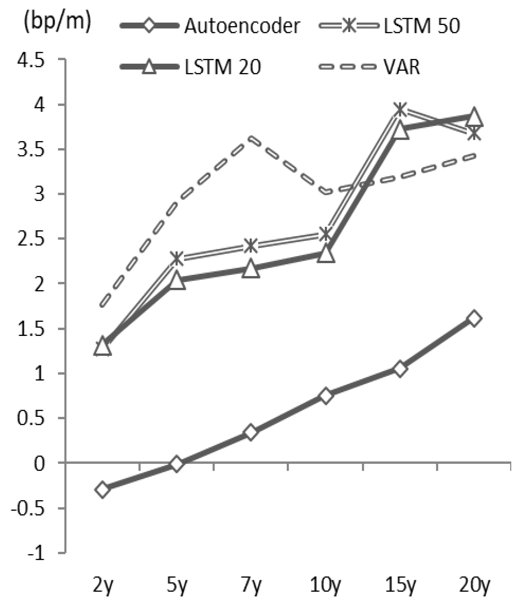
Figure 19 shows the results of our investment simulation. Similar to the strategy using the autoencoder, the learning period of the LSTM and VAR model is 5 years, and we relearn the model every year. As a result, the investment strategy using these models demonstrates relatively high investment performance compared to that of the strategy using the autoencoder.

Considering the cumulative returns presented in Figure 20, the LSTM and VAR model utilizing the historical time series information provides stable forecasting of the returns. On the other hand, the strategy using the autoencoder that does not use time series information of past interest rates as the input data is inferior in terms of trading performance.

However, based on the yield curve shape information at the time of investment, the autoencoder determines if the government bonds are overpriced or underpriced, enabling a decision to sell or buy based on its valuation. The cumulative return of the autoencoder strategy is stably positive. So, the evaluation of overpricing or underpricing for each bond at the time of investment is reasonable. Therefore, the proposed model using an autoencoder is effective from the viewpoint of the asset evaluation of government bonds relative to the market environment.

In addition, from the viewpoint of interpretability, we have merit to use the autoencoder-based model that we propose in this research. The autoencoder-based model expresses the yield curve by three factors, which are interpreted as the level, slope, and curvature of the yield curve. In the trading strategy, as we proposed, we decide to sell or buy based on its valuation of the yield curve shape information at the time of investment based on the autoencoder. So, the proposed strategy is to construct a trading position to the direction in which the deviation between the actual curve and the theoretical curve by autoencoder is corrected. Therefore, we can clearly interpret what we are betting on in the proposed strategy. On the other hand, the investment strategy based on LSTM and VAR shown in the paper predicts the future interest rate directly based on historical interest rate information at the time of investment and decide to sell or buy based on prediction. Therefore, it is difficult to interpret whether the trading position by LSTM or VAR is betting on the pattern of interest rate change from the past or betting on correcting the distortion of the yield curve at the time of investment. As described above, the merit of the proposed model based on the autoencoder is the interpretability of the model and the interpretability of what we are betting on.

Finally, I would like to supplement the analysis/simulation programming method used in this research. The programming language used throughout this research is Python, and the Python library TensorFlow was used to implement the neural network (the proposed autoencoder-based yield curve model, LSTM model), and scikit-learn was used to implement PCA.

5. Conclusions

We proposed a factor model for JGB yield curves by using an autoencoder. In Japan, the shape of the yield curve has changed significantly in recent years following major adjustments in monetary policy, such as the “Quantitative and Qualitative Monetary Easing with Yield Curve Control” by the BOJ in 2016. Under such monetary policy, the medium-term and short-term interest rates of JGBs are currently negative. Recently, interest rates have been declining due to the slow growth of the global economy, and interest rates have become negative in some countries other than Japan due to the central banks’ monetary easing. In addition to adjusting short-term policy rates, some central banks have also introduced policies that directly affect long-term interest rates, such as the purchase of long-term government bonds. As a result, the shape of the yield curve has been diversified globally. So, there is now an increasing need for a yield curve model that can flexibly cope with these changing yield curve shapes. The neural network-based autoencoder model offers flexibility to represent the shape of the yield curve by configuring the number of nodes and the activation function.

When a complex neural network model, such as deep learning, is used, the interpretability of the model and output results is often difficult. In this research, we focused on the model parameters of the intermediate layer of the neural network that constitute the autoencoder and confirmed that the three automatically generated factors represent the “Level,” “Curvature,” and “Slope” of the yield curve. We think this interpretation of the yield curve model is significant from the viewpoint of risk management in financial businesses.

Furthermore, we developed a long–short strategy for JGBs by using the autoencoder to determine if they are overpriced or underpriced, and we confirmed the good performance of this approach relative to the trend-follow investment strategy. In particular, for the 10-year and 20-year government bonds, the cumulative return of the one-month investment strategy based on the autoencoder-based model (three hidden layer node model with a learning period of 5 years) is stably positive. So, we see that the evaluation of overpricing or underpricing for each bond at the time of investment is reasonable in these cases. Therefore, our proposed model using an autoencoder is effective for asset evaluation of long-term government bonds relative to the market environment.

On the other hand, for prediction accuracy, the LSTM model using past interest rate time series data offered better performance. Based on this result, future work will customize the neural network structure of the yield curve model to improve the prediction accuracy in addition to the interpretability that we proposed here. Furthermore, we analyzed interest rate data in the Japanese government bond market, and, in the future, we will conduct similar analyses on other market data, such as in the United States and Europe, as well as compare global market analyses.

References

1. Abe, Masaya, and Hideki Nakayama. 2018. Deep Learning for Forecasting Stock Returns in the Cross-Section. Paper presented at Pacific-Asia Conference on Knowledge Discovery and Data Mining, Melbourne, VIC, Australia, June 3–6; pp. 273–84. [Google Scholar]
2. Afonso, António, and Manuel M.F. Martins. 2012. Level, slope, curvature of the sovereign yield curve, and fiscal behaviour. Journal of Banking & Finance 36: 1789–807. [Google Scholar]
3. Ang, Andrew, and Monika Piazzesi. 2003. A no-arbitrage vector autoregression of term structure dynamics with macroeconomic and latent variables. Journal of Monetary Economics 50: 745–87. [Google Scholar] [CrossRef]
4. Bank of Japan. 2016. New Framework for Strengthening Monetary Easing: “Quantitative and Qualitative Monetary Easing with Yield Curve Control”. Available online: https://www.boj.or.jp/en/announcements/release_2016/k160921a.pdf (accessed on 20 December 2019).
5. Dai, Qiang, and Kenneth J. Singleton. 2000. Specification analysis of affine term structure models. Journal of Finance 55: 1943–78. [Google Scholar] [CrossRef]
6. Diebold, Francis X., and Canlin Li. 2006. Forecasting the term structure of government bond yields. Journal of Econometrics 130: 337–64. [Google Scholar] [CrossRef] [Green Version]
7. Diebold, Francis X., Glenn D. Rudebusch, and S. Boragan Aruoba. 2006. The macroeconomy and the yield curve: A dynamic latent factor approach. Journal of Econometrics 131: 309–38. [Google Scholar] [CrossRef] [Green Version]
8. Estrella, Arturo, and Frederic S. Mishkin. 1997. The predictive power of the term structure of interest rates in Europe and the United States: Implications for the European Central Bank. European Economic Review 41: 1375–401. [Google Scholar] [CrossRef]
9. Hinton, Geoffrey E., and Ruslan Salakhutdinov. 2006. Reducing the Dimensionality of Data with Neural Networks. Science 313: 504–7. [Google Scholar] [CrossRef] [Green Version]
10. Hochreiter, Sepp, and Jürgen Schmidhuber. 1997. Long Short-Term Memory. Neural Computation 9: 1735–80. [Google Scholar] [CrossRef]
11. Kikuchi, Kentaro, and Kohei Shintani. 2012. Comparative Analysis of Zero Coupon Yield Curve Estimation Methods Using JGB Price Data. In IMES Discussion Paper Series 2012-E-4. Tokyo: Institute for Monetary and Economic Studies Bank of Japan. [Google Scholar]
12. Krauss, Christopher, Xuan Anh Do, and Nicolas Huck. 2017. Deep neural networks, gradient-boosted trees, random forests: Statistical arbitrage on the S&P 500. European Journal of Operational Research 259: 689–702. [Google Scholar]
13. Ludvigson, Sydney C., and Serena Ng. 2009. Macro Factors in Bond Risk Premia. The Review of Financial Studies 22: 5027–67. [Google Scholar] [CrossRef] [Green Version]
14. Matthew, Dixon, Klabjan Diego, and Bang Jin Hoon. 2017. Classification-based financial markets prediction using deep neural networks. Algorithmic Finance 6: 67–77. [Google Scholar]
15. McCulloch, J. Huston. 1971. Measuring the Term Structure of Interest Rates. The Journal of Business 44: 19–31. [Google Scholar] [CrossRef]
16. McCulloch, J. Huston. 1975. The Tax-Adjusted Yield Curve. The Journal of Finance 30: 811–30. [Google Scholar] [CrossRef]
17. Ministory of Finance. 2019. Japan, Interest Rate Historical Data. Available online: https://www.mof.go.jp/english/jgbs/reference/interest_rate/index.htm (accessed on 7 December 2019).
18. Moench, Emanuel. 2008. Forecasting the yield curve in a data-rich environment: A no-arbitrage factor-augmented VAR approach. Journal of Econometrics 146: 26–43. [Google Scholar] [CrossRef]
19. Nelson, Charles, and Andrew F. Siegel. 1987. Parsimonious Modeling of Yield Curves. The Journal of Business 60: 473–89. [Google Scholar] [CrossRef]
20. Olson, Dennis, and Charles Mossman. 2003. Neural network forecasts of Canadian stock returns using accounting ratios. International Journal of Forecasting 19: 453–65. [Google Scholar] [CrossRef]
21. Reisman, Haim, and Gady Zohar. 2004. Short-Term Predictability of the Term Structure. The Journal of Fixed Income 14: 7–14. [Google Scholar] [CrossRef]
22. Soni, Sneha. 2011. Applications of ANNs in stock market prediction: A survey. International Journal of Computer Science & Engineering Technology 2: 71–83. [Google Scholar]
23. Steeley, James M. 1991. Estimating the Gilt-Edged Term Structure: Basis Splines and Confidence Intervals. Journal of Business Finance and Accounting 18: 513–29. [Google Scholar] [CrossRef]
24. Schaefer, Stephen M. 1981. Measuring a Tax-Specific Term Structure of Interest Rates in the Market for British Government Securities. The Economic Journal 91: 415–38. [Google Scholar] [CrossRef]
25. Suimon, Yoshiyuki. 2018. Fluctuation Model of JGB Yield Curve Using Machine Learning and The Interest Rate Prediction. Tokyo: The Japanese Society for Artificial Intelligence, SIG-FIN, pp. 46–49. [Google Scholar]
26. Suimon, Yoshiyuki, Hiroki Sakaji, Kiyoshi Izumi, Takashi Shimada, and Hiroyasu Matsushima. 2019a. JGB Long-Term Interest Rate Forecast Considering the Connection Between the Japanese and US Yield Curve. Tokyo: The Japanese Society for Artificial Intelligence, SIG-FIN, pp. 81–87. [Google Scholar]
27. Suimon, Yoshiyuki, Hiroki Sakaji, Kiyoshi Izumi, Takashi Shimada, and Hiroyasu Matsushima. 2019b. Japanese long-term interest rate forecast considering the connection between the Japanese and US yield curve. Paper presented at IEEE Conference on Computational Intelligence for Financial Engineering and Economics, Shenzhen, China, May 4–5. [Google Scholar]
28. Suimon, Yoshiyuki, Hiroki Sakaji, Kiyoshi Izumi, Takashi Shimada, and Hiroyasu Matsushima. 2019c. Extraction of relationship between Japanese and US interest rates using machine learning methods. Paper presented at International Conference on Smart Computing and Artificial Intelligence, Toyama, Japan, July 7–11. [Google Scholar]
29. Svensson, Lars E.O. 1995. Estimating forward interest rates with the extended Nelson and Siegel method. Sveriges Riksbank Quarterly Review 3: 13–26. [Google Scholar]
30. Tanggaard, Carsten. 1997. Nonparametric Smoothing of Yield Curves. Review of Quantitative Finance and Accounting 9: 251–67. [Google Scholar] [CrossRef]
31. Yu-cho Foundation. 2018. Research on the Government Bond Market. Tokyo: Postal Savings Assets Research Center Yu-Cho Foundation. [Google Scholar]
Figure 1. Japanese government bond (JGB) yield curve.
Jrfm 13 00082 g001
Figure 2. Historical data of Japanese government bond interest rates.
Jrfm 13 00082 g002
Figure 3. Japanese government bond (JGB) yield curve data and the Nelson–Siegel model curve.
Jrfm 13 00082 g003
Figure 4. Three factors of the Nelson–Siegel model.
Jrfm 13 00082 g004
Figure 5. Eigenvectors of the principal component analysis (PCA) factors 1–3.
Jrfm 13 00082 g005
Figure 6. Autoencoder model constructed with interest rate data.
Jrfm 13 00082 g006
Figure 7. Coefficients of the linear function output from the hidden layer (for three nodes).
Jrfm 13 00082 g007
Figure 8. Plots of the hidden layer node output with the corresponding interest rate levels and interest rate spread.
Jrfm 13 00082 g008
Figure 9. Coefficients of the linear function output from the hidden layer with two nodes.
Jrfm 13 00082 g009
Figure 10. Plots of the hidden layer nodes’ output corresponding to the interest rate spreads.
Jrfm 13 00082 g010
Figure 11. Coefficients of the linear function output from the hidden layer with four nodes.
Jrfm 13 00082 g011
Figure 12. Judgments of overvaluation or undervaluation using an autoencoder.
Jrfm 13 00082 g012
Figure 13. Average monthly capital gains based on different learning periods on a three-node hidden layer model with investment periods of 1 or 3 months.
Jrfm 13 00082 g013
Figure 14. Monetary policy change with the medium- and short-term interest rates.
Jrfm 13 00082 g014
Figure 15. Interest rates and the result of the autoencoder-based investment strategies.
Jrfm 13 00082 g015
Figure 16. The differences in interest rate information used for each investment strategy.
Jrfm 13 00082 g016
Figure 17. Structure of the Long Short-Term Memory (LSTM) model.
Jrfm 13 00082 g017
Figure 18. Structure of the LSTM block.
Jrfm 13 00082 g018
Figure 19. Average monthly capital gains using the LTSM, VAR and autoencoder-based models’ learning period of 5 years and an investment period of 1 month.
Jrfm 13 00082 g019
Figure 20. Cumulative returns from each investment strategy.
Jrfm 13 00082 g020