Contracts for Difference: A Reinforcement Learning Approach

Abstract

We present a deep reinforcement learning framework for an automatic trading of contracts for difference (CfD) on indices at a high frequency. Our contribution proves that reinforcement learning agents with recurrent long short-term memory (LSTM) networks can learn from recent market history and outperform the market. Usually, these approaches depend on a low latency. In a real-world example, we show that an increased model size may compensate for a higher latency. As the noisy nature of economic trends complicates predictions, especially in speculative assets, our approach does not predict courses but instead uses a reinforcement learning agent to learn an overall lucrative trading policy. Therefore, we simulate a virtual market environment, based on historical trading data. Our environment provides a partially observable Markov decision process (POMDP) to reinforcement learners and allows the training of various strategies.

1. Introduction

High-frequency trading (HFT) causes a high proportion of market activity but receives only little academic attention Aldridge (2013); Brogaard (2010). Artificial intelligence applications, especially machine learning algorithms, offer new perspectives, possibilities and tools for economic modelling and reasoning Aghion et al. (2017). In particular, high-frequency trading of speculative assets like Contracts for Difference (CfD) relies on a statistically appropriate, automated handling of risk. Therefore, we simulate a derivative market as a partially observable Markov decision process (POMDP) for Reinforcement Learning of CfD trading policies at high frequency.

To determine a reward for the agent action, the environment evaluates the trade action on historical market data and returns the financial profit or loss. The agent then tries to find an optimal policy that maximizes the expected rewards. To approximate an optimal policy, we use deep neural networks and evaluate both a feedforward neural network and a recurrent long short-term memory network (LSTM). As a reinforcement learning method, we propose a Q-Learning approach with prioritized experience replay. To evaluate the real-world applicability of our approach, we also perform a test under real market conditions.

We begin this paper by introducing Contracts for Differences and presenting relevant state-of-the-art research in Section 2. In Section 3, we explain our implementation in detail and in Section 4 we illuminate our evaluation process and the results we obtained. The conclusion in Section 6 ends this paper with a summary, a short discussion and possible future work.

Contracts for Difference

A contract for Difference (CfD), a form of a total return swap contract, allows two parties to exchange the performance and income of an underlying asset for interest payments. In other words, economic players may bet on rising or falling prices and profit, if the real price development matches their bet. Due to the possibility of highly leveraged bets, high wins may occur as well as high losses.

In contrast to other derivatives, such as knockout certificates, warrants or forward transactions, a CfD allows the independent setting of stop-loss and take-profit values. Setting a take-profit and stop-loss value automatically closes the deal, if the underlying course strikes the corresponding threshold. If the asset development does not correspond to the bet, but develops in the opposite direction, a depth arises which can lead to additional financing obligations. A security deposit, also referred to as a margin, fulfils the purpose of hedging the transaction. Since additional funding obligations in the event of default can easily exceed the margin, individual traders can suffer very high losses in a very short time if they have not set a stop-loss value.

Concerning legal aspects, CfD trading currently faces an embargo in the United States of America. According to a general ruling of the Federal Financial Supervisory Authority (Bundesanstalt für Finanzdienstleistungsaufsicht), a broker in Germany may only offer such speculative options to his customers, if they have no additional liability in case of default, but instead only lose their security deposit.

2. State of the Art

State-of-the-art stock market prediction on longer time scales usually incorporates external textual information from news feeds or social media Bollen et al. (2011); Ding et al. (2015); Vargas et al. (2017). Using only historical trade data, Chen et al. (2015) investigates a LSTM-based course prediction model for the Chinese stock market to predict rising or falling courses on daily time scales, which achieves accuracies between $64.3\%$ and $77.2\%$. A deep learning LSTM implementation by Akita et al. (2016) learns to predict stock prices based on combined news text together and raw pricing information, allowing for profitable trading applications.

Considering high-frequency trading algorithms and strategies, a vast variety of applications exists, including many classic machine learning approaches Aldridge (2013). Concerning reinforcement learning in high-frequency trading, Moody and Saffell (1999) proposed a reinforcement learning system to optimize a strategy that incorporates long, short and neutral positions, based on financial and macroeconomic data. There also exist reinforcement learning approaches for high-frequency trading on foreign exchange markets with deep reinforcement learning Dempster and Romahi (2002); Gold (2003); Lim and Gorse (2018).

Yet, to the best of our knowledge, no deep reinforcement learning research for high-frequency trading on contracts for difference exists.

3. Method

We aim to find optimal trading policies in adjustable environment setups, using Q-Learning, as proposed by Watkins and Dayan (1992). To boost the training efficiency, we employ a prioritized experience replay memory for all our models Schaul et al. (2015). We use AdaGrad updates as a weight update rule Duchi et al. (2011). As for an observed state s, the underlying POMDP presents a tick chart of length l. The tick chart consists of a sequence of ask and bid prices, with the corresponding ask and bid trade volumes. We denote the price values per tick as $p_{ask},p_{bid}$ and the trade volumes as $v_{ask},v_{bid}$.

3.1. Models

We investigate both a feedforward and a LSTM architecture. Both architectures feature the same input and output layers setup, but have different hidden layers. The input layer contains the state s, in form of a tick data sequence with length l. As for the output layer, the neural network approximates the Q-values $Q(s,a)$ for each action in the action space $a\in A$. To approximate these values, we use an output layer of $\left|A\right|$ neurons, each neuron with linear activation. Each action $a\in A$ may invoke a different trade order.

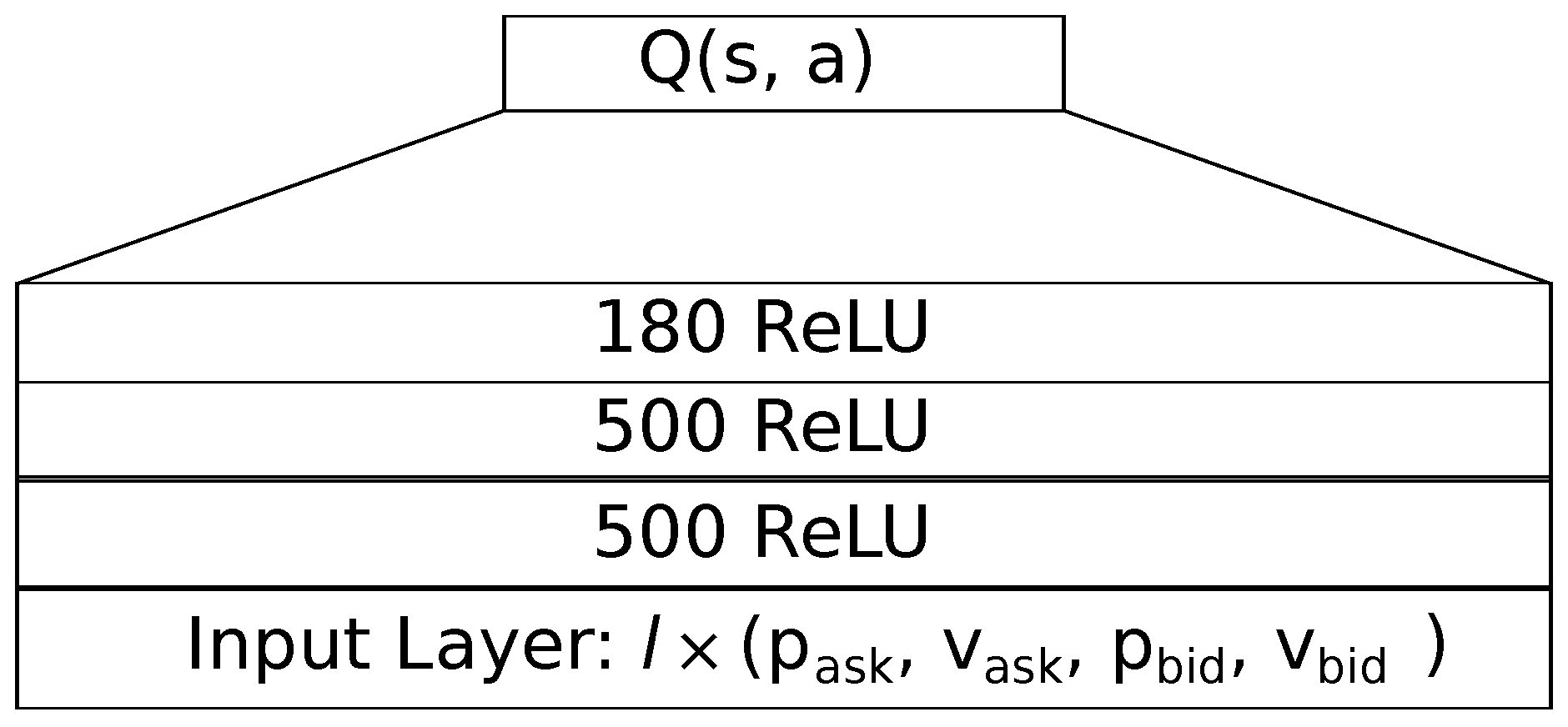
3.1.1. Feedforward

Our feedforward neural network features a hidden part of three dense layers, as sketched in Figure 1. The first two dense layers consist of 500 rectifying linear units with a small bias of $0.1$. We use the He weight initialization with a uniform distribution to initialize the weights. To obtain a roughly the same number of weights as we have in our LSTM architecture, we append a third layer with 180 rectifying linear units, also with a bias of $0.1$. For an input length of $l=500$ and an action space size of $\left|A\right|=3$, the feedforward network has a total of 840,540 parameters.

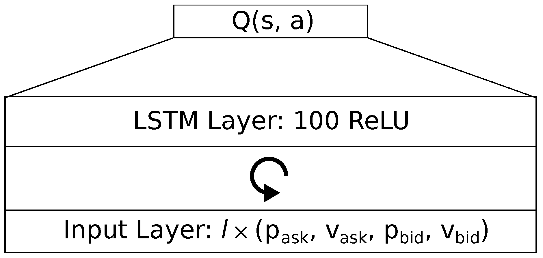
3.1.2. LSTM

We use a LSTM network with forget gates as proposed by Gers et al. (1999). Like for the feedforward network, the input layer consists of a sequence of trade data. During training and testing, we keep the sequence length constant. The output layer approximates the linear Q-Values, using the hidden state of the LSTM layer, inspired by an architecture found in Mirowski et al. (2016). The hidden LSTM layer consists of a single recurrent layer with 100 rectifying linear units, as shown in Figure 2. We initialize the gates weights using the normal distribution. For a fixed input length of $l=500$ and an action space size of $\left|A\right|=3$, the LSTM network has a total of 840,300 parameters.

3.2. Environment

We implement a simple market logic that operates on historical trading data on a tick time scale as a basis for a POMDP. The environment processes the agents trading actions without a delay, which simplifies analytical investigations but discards the important factor of latency. To increases the information content presented to the agent in each observation, we remove equal successive ticks. This results in a reduced input sequence length but discards the information about how long a particular state lasts.

As a state s, the environment presents a sequence of l unique ticks, starting from a random point t in trade history x. We adjust each state for the mean value:

$$s=X[t:t+l]-\overline{x}[t:t+l]$$

For each state s, the agent chooses an action a. If the agent chooses the action $a=0$ to open no trade, the agent receives a reward of 0 and observes the next state. An episode in this environment terminates if the agent chooses to open a deal with an action $a\ne 0$. When the agent performs an action, the simulation runs forward until the market price reaches either the take-profit or the stop-loss value. The environment then returns the achieved financial profit or loss as a reward, scaled by a constant factor. The pseudo codes in the Appendix A describe the whole training algorithm for a Q-Learning agent on a simulated CfD market.

4. Evaluation

To evaluate our approach, we use a DE30 CfD index with a nominal value of €25 per lot at a $5\%$ leverage. We reflect the boundary conditions of the chosen asset in our simulation by setting an adequate reward scaling factor. A small trade volume of $0.01$ lot leads to a reward scaling factor of $c=0.25$ for the training and testing procedure.

As a data basis for our market simulation, we have recorded the corresponding market history from July 2019, using the interface provided by X Open Hub xAPI (n.d.). We recorded five data points per second and removed unchanged successor data points. After recording for a month, we have split the data into a set for the training simulation and a set for the test simulation. This led us to a data basis of about three million unique tick values for the training environment, and about half a million unique ticks for the market logic in our testing procedure.

In this evaluation, we use the models as described in Section 3 with an action space of size $\left|A\right|=3$. The action $a=0$ does not cause a trade order but makes the agent wait and observe the next tick. To open a long position, the agent would choose $a=1$, while the action $a=2$ would cause the opening of a short position.

To find good training parameters for our models, we have conducted a grid search in a space of batch size, learning rate and input sequence length. We evaluate batch sizes $b\in \{10,50,100\}$, learning rates $\eta \in \{{10}^{-4},{10}^{-5},{10}^{-6}\}$ and input sequence lengths $l\in \{50,100,250\}$. By comparing the final equities after 1000 test trades we find an optimal parameter configuration. For the feedforward architecture, we find the optimal training parameter configuration in $(b=100,l=50,\eta ={10}^{-5})$. Concerning the single layer LSTM network, we find the best test result for in $(b=10,l=50,\eta ={10}^{-4})$.

4.1. Training

For each memory record, we have a starting state $s_1$, the chosen action a, the follow-up state $s_2$ alongside with the achieved reward r and a variable e. The variable e tells us if the replayed experience features a closed trade, thereby ending in a terminal state. In a training run, the agent performs a total of 250,000 learning steps. For each learning step, we sample a batch of b independent experiences $(s_1,a,s_2,r,e)$ from the prioritized replay memory. Then, we apply an AdaGrad weight update to the neural network, based on the difference between the predicted and the actual Q-values. On a currently standard workstation, the training of the smallest feedforward model takes about 15 min, while the training of the large two layer LSTM model took about two days, using an implementation in Theano and Lasagne Dieleman et al. (2015); Theano Development Team (2016).

4.2. Test

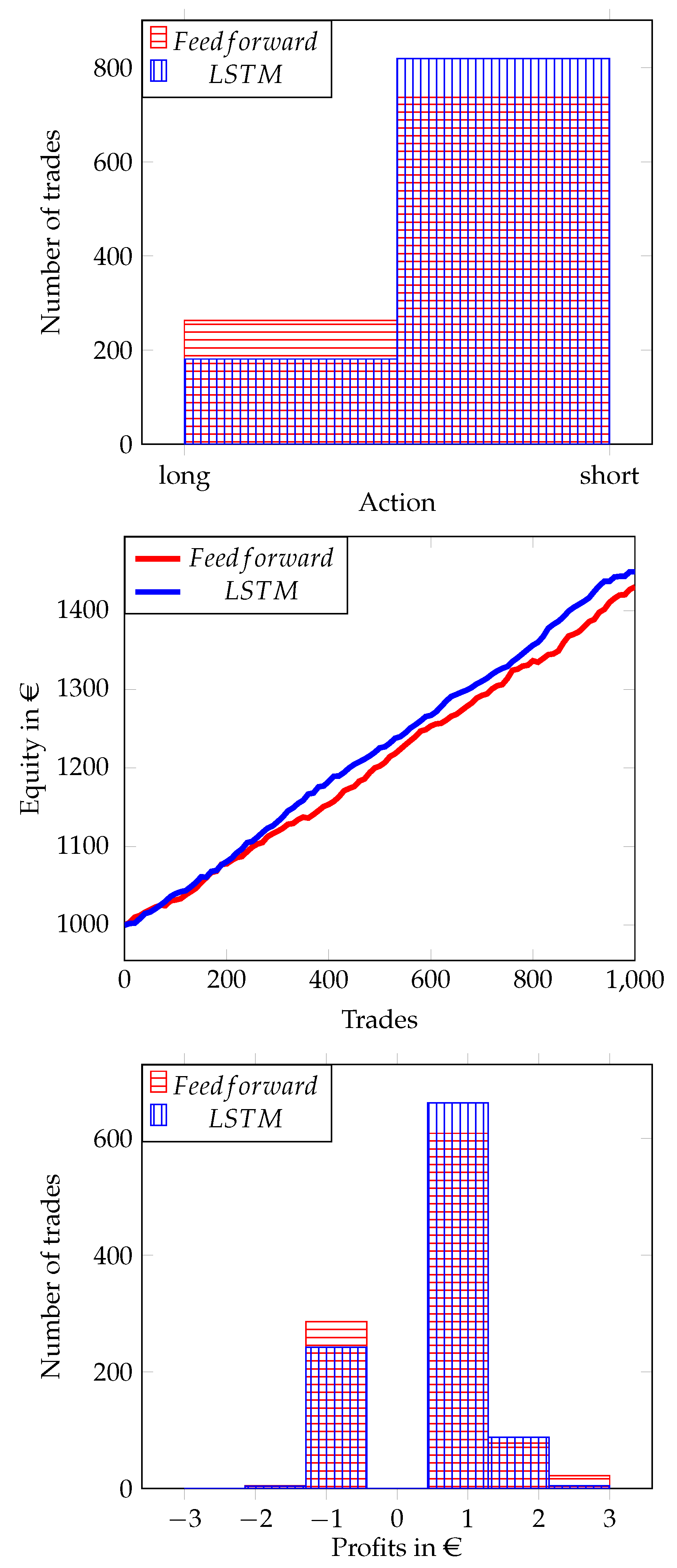
To evaluate our models, we perform tests on unseen market data. If for an optimal action a the expected reward $Q(s,a)<0$, the agent does not execute the order, as we want our agent to achieve a profit and not a minimal loss. This increases the time between trades at the benefit of more likely success. We test each feedforward and LSTM network by performing a total of 1000 test trades on unseen data. Each test run starts with an equity of €1000.

From the action distribution in Figure 3, we can see that both the feedforward and the LSTM agent tend to open short positions more frequently. To perform a trade, the feedforward network observes for 2429 ticks on average, while the LSTM network waits for 4654 tick observations before committing to any trade action. While the LSTM network tends to wait and observe, by choosing the action $a=0$ more frequently, the feedforward network makes decisions faster. We can see an increase in equity for both our models in Figure 3. Furthermore, the LSTM network seems to have a conceptual advantage due to its immanent handling of sequences. Looking at the differences in the profit distribution, as shown in Figure 3, we find that the LSTM network achieves lower profits.

5. Real-World Application

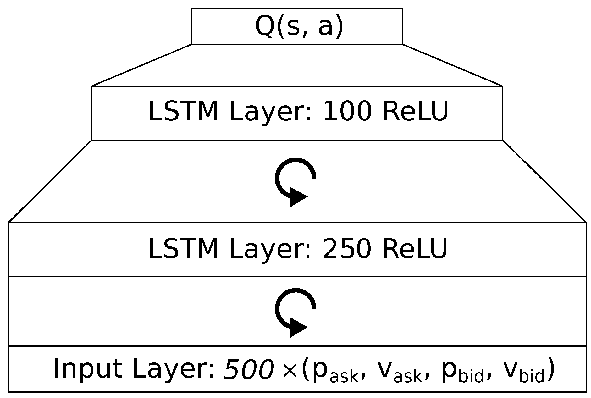
For a real-world proof of concept with a demo account, we use an LSTM architecture as it seems to outperform a feedforward network. At first, we tried to apply the best model we found without further boundary conditions. The latency issues caused the agent to decide upon a past observation, lowering the temporal precision and causing more negative profits. Also, the agents orders come to pass late, such that the state has already changed and the agent misses its intended price to set the take-profit and stop-loss values.

To accommodate for the latency problems, we have designed an LSTM architecture with an additional layer of 250 LSTM units, as shown in Figure 4. Also, we increased the action space size to $A=\left|10\right|$ and introduce a function $\delta =d_{profit}\left(a\right)$ to map a to a certain $\delta$ to add to the stop-loss and take-profit values, thus allowing the anticipation of high spreads:

$$d_{profit}\left(a\right):=\left\{\begin{array}{cc}\delta =0,\hfill & :a=0\hfill \\ \delta =2,\hfill & :a=1,a=6\hfill \\ \delta =5,\hfill & :a=2,a=7\hfill \\ \delta =10,\hfill & :a=3,a=8\hfill \\ \delta =25,\hfill & :a=4,a=9\hfill \\ \delta =50,\hfill & :a=5,a=10\hfill \end{array}\right.$$

This workaround introduced some slack into the strategy to accommodate for the various problems introduced by latency. Conceptually, these adjustable delta values allow the agent to anticipate different magnitudes of price changes. This decreases the risk of immediate default, but potentially leads to a high loss.

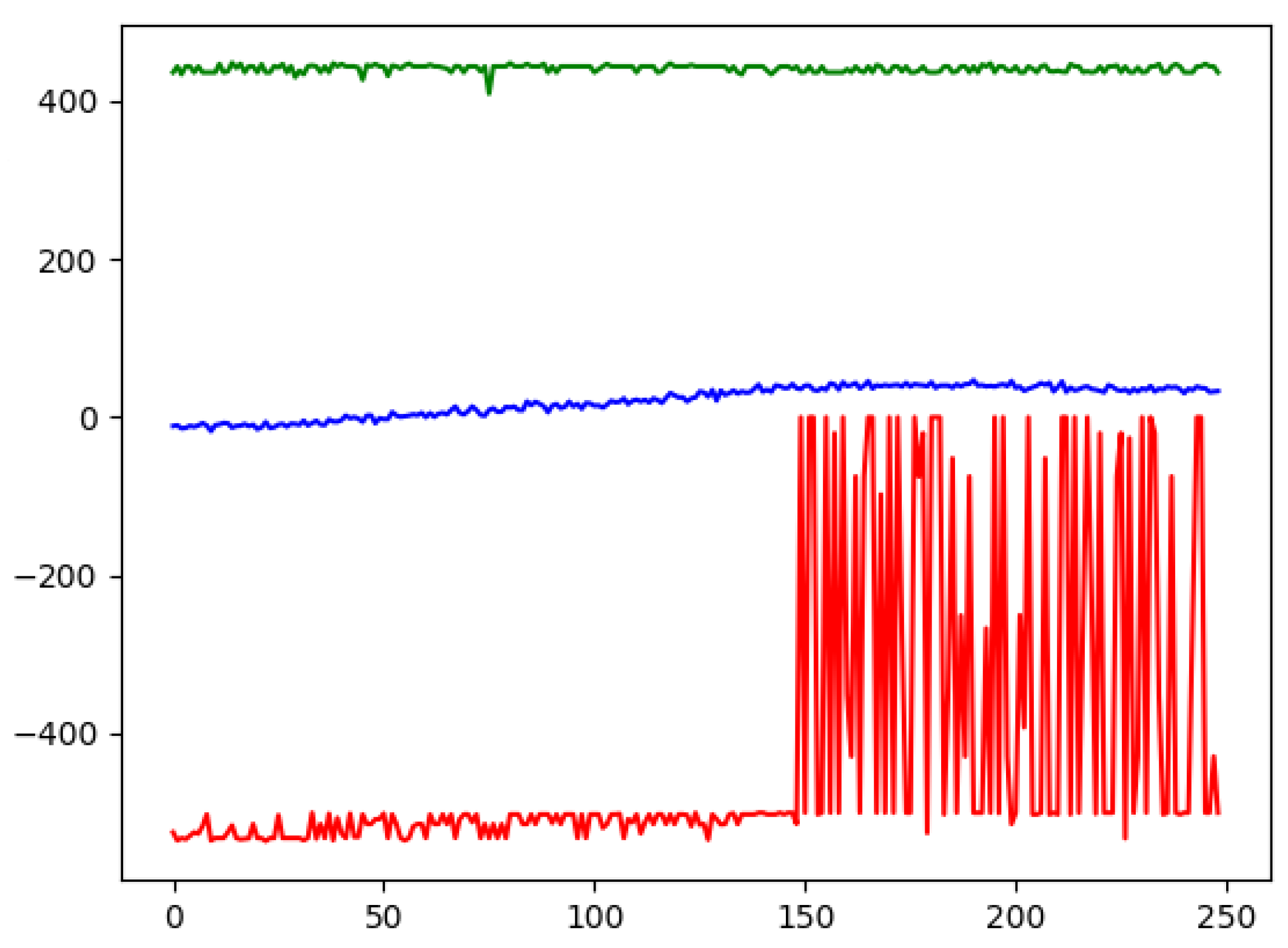
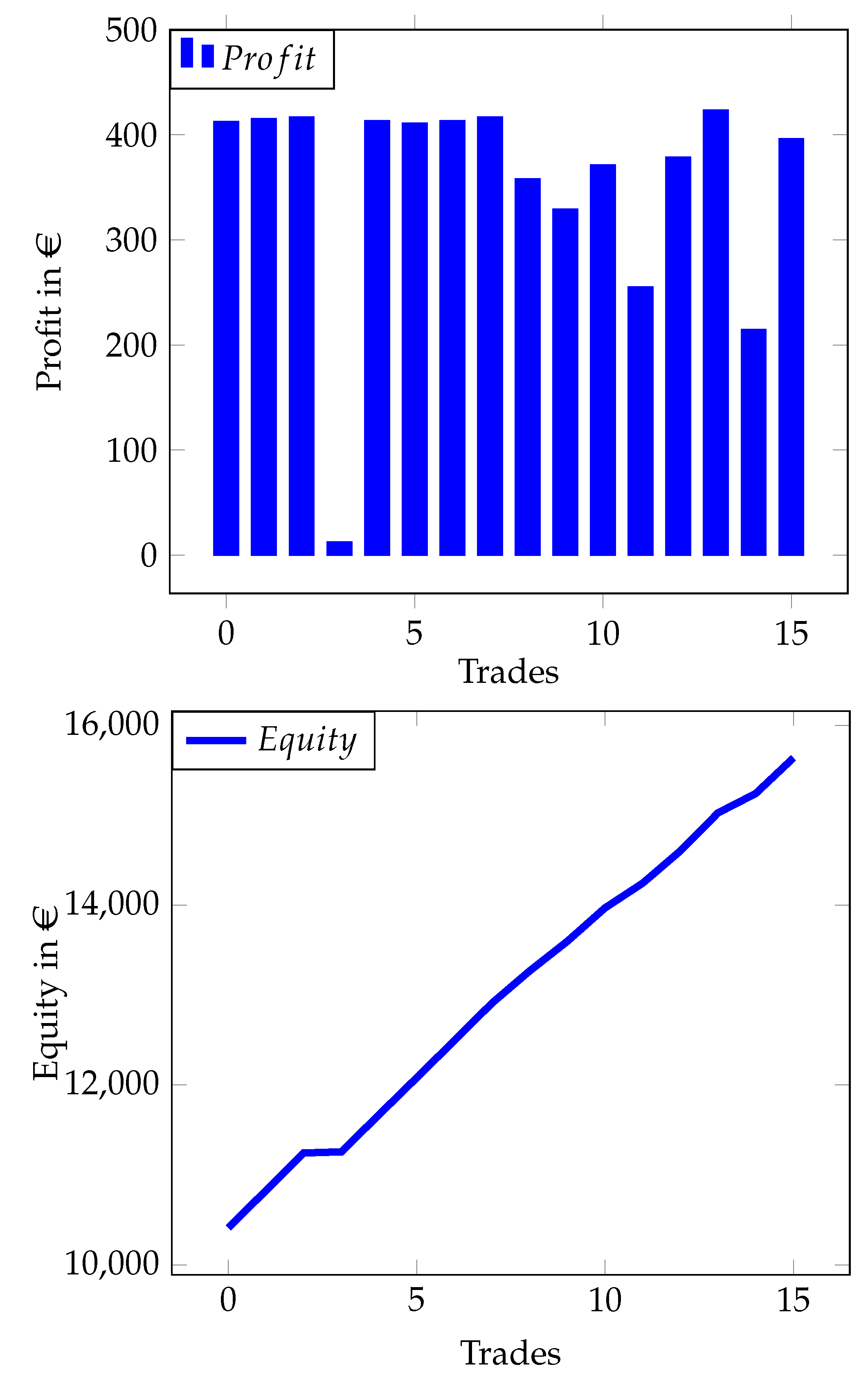
Using these settings, we have trained the LSTM network with a training parameter configuration of $(b=50,l=250,\eta ={10}^{-5})$. In the corresponding learning dynamics, as shown Figure 5, we can see that the agents maintain potential high wins while trying to reduce losses, which result in an overall surplus during training. To keep the agent up to date with the real-world market data, we have trained the network out of trading time. We let our real-world test run for ten trading days, in which the agent opened and closed 16 trades without manual interference. Also, we superimpose a rule-based hedging system, which allows the agent to open one long position, one short position and a third arbitrary position. contemporaneous. Figure 6 shows the profits achieved by the agent and the corresponding increase in equity.

6. Discussion

Comparing the results of the recurrent LSTM network to the simple feedforward network, we can state that assuming sequences in trading data may slightly improve results of a machine learning system. Although our contribution proves that artificially intelligent trading automata may learn different strategies, if given an appropriate training environment, we did not investigate the effects of changing the training environment. We did not investigate the effect of adjusting the chance-risk-ratio at training time, neither did we study the effect of larger replay memory sizes or other learning schemes than Q-Learning. Instead of using batch normalization with a division by the standard deviation, we only subtracted the mean value.

We did not compare our method to related concepts, as presented in the state-of-the-art section, and leave the comparison of different baselines for future research. As for now, we have only considered the course data of a single trading symbol.

As for the real-world example, we have used a demo account with a limited validity of only 20 trading days. We could only use ten trading days for testing our approach in a real-world setting. That said, we did not observe enough trades to make a reliable statement about the long-term reliability of that concrete strategy in a real-world setting.

6.1. Future Work

To do a baseline comparison research, a market simulation needs an interface that can provide its state data in various representations and interpret different kind of order types. Such an environment also needs to provide trading logic for various assets as well as their derivatives. Also, a simulated market environment for a baseline comparison may consider the market effects of trades.

Considering our simulated market, we may improve the environment in various ways. First, the introduction of an artificial latency would allow experiments that take high-frequency trading requirements into account. This would allow the simulation of various agents that compete under different latency conditions. Secondly, we may gather input data from more than one asset to make use of correlations. And third, we currently neglect the influence of the agents trading decisions on the price development.

In future work, we may study the benefit of aggregated input sequences of different assets, for example a composite input of gold, oil, index charts and foreign exchange markets. We may also provide the input on different temporal solutions, for example on a daily, monthly, or weekly chart. A convolutional neural network may correlate course data from different sources, in order to improve the optimal policy. Given a broader observation space, a reinforcement learning agent may also learn more sophisticated policies, for example placing orders on more than one asset. More sophisticated methods of transfer learning may enable us to reuse already acquired knowledge to improve the performance on unknown assets. For instance, we may use progressive neural networks to transfer knowledge into multiple action spaces. This allows the learning of trading on multiple assets simultaneously, making use of correlations in a large input space.

Furthermore, future work may consider the integration of economic news text as input word vectors. This way, the trade proposals made by our agents may serve as an input for more sophisticated trading algorithms that employ prior market knowledge. As an example, a rule-based system that incorporates long-term market knowledge may make use of the agent proposals to provide a fully automatic, reliable trading program. Such a rule-based system might prevent the agent to open positions if above or below a certain threshold that a human operator may set according to his or her prior knowledge of the market.

6.2. Conclusions

To conclude, our studies prove that there is a high-frequency trading system which, in a simulation, critically outperforms the market, given a near-zero latency. Our real-world application shows that additional model parameters may compensate for a lower latency. We have contributed a parametrizable training environment that allows the training of such reinforcement learning agents for CfD trading policies. Our neural network implementations serve as a proof of concept for artificially intelligent trading automata that operate on high frequencies. As our approach conceptually allows the learning of trading strategies of arbitrary time scales, a user may provide minutely, hourly or even daily closing prices as a data basis for training as well.

Another key observation of our investigation reveals the importance of using a training setup that matches the real trading conditions. Furthermore, we observe that if we perform trades without setting stop-loss values, the CfD remains open at a position that matches the our obersvations of resistance lines on the index price.