1. Introduction
The recent complexity of financial technology has increased the risk of financial markets, especially systemic risks. A systemic risk comes from the interaction between various components in financial markets. Systemic risk is one of the most significant dangers in financial markets because small triggers cause huge shocks in financial markets with the existence of systemic risks.
One famous example of systemic risk is the financial crisis of 2007–2008. The crisis began with a local default of American subprime mortgage loans. However, the fails in subprime mortgages spread widely, and it also affected stock markets. Moreover, it affected not only American financial markets but also global financial markets.
The other example of those risks is flash crashes. One of the most famous flash crash was the 2010 Flash Crash in the U.S. stock market on 6 May 2010. S&P 500 and Dow Jones Industrial Average rapidly dropped. The main reason for this crash was said to be one big sell order. Additionally, many algorithmic sell orders followed the first big sell orders, and it was said to cause a significant crash. Supposedly, improvements in information technologies contributed to risks in the financial market. However, the ground truth of these crashes has not been revealed.
These systemic risks should be reduced to stabilize financial markets. Once the risk becomes a reality and causes shocks, the spreading of shocks could not be stopped with a small amount of effort. Even if the beginning could be identified, it would be almost impossible to cut the chain of failures. It is because the risks and shocks come from the complex structure of financial markets. To avoid these shocks, some regulations or structural improvement in financial markets is necessary beforehand.
Therefore, predicting and identifying potential risks and making regulations for them are essential for market stabilization. Of course, it is also essential to learn from what happened before.
In terms of predicting and identifying potential risks, there are many ways to do so using artificial intelligence (AI) technologies. One of the most significant approaches to identify the potential risks is simulations. Simulation is also one of AI technologies and a promising approach. Simulation can test hypothetical situations and run again and again. It is different from the real financial market and beneficial.
Especially, agent-based simulation is useful for social science (
Moss and Edmonds 2005). Agent-based simulations aim to imitate the real world by making an imaginary world with agents on computers.
Moreover, one promising approach of agent-based simulations for financial markets is artificial market simulations. In this simulation, agents are constructed by imitating traders in the real financial market. In some previous work, such as
Mizuta et al. (
2016);
Torii et al. (
2015), this type of approach was used. In addition,
Mizuta (
2019) argued that artificial market simulation could contribute to the improvements of the structures or rules and regulations of financial markets.
In terms of regulations, there is a well-known regulation called “Basel regulatory framework.” This regulatory framework has been updated and still active for over three decades in financial markets. This series of regulations was started as “Basel I” in 1988. In 1996, modified Basel I was agreed upon (
Basle Committee on Banking Supervision 1996a). This regulatory framework included market operation risks for the first time. After the agreement of Basel II and modifications of it, the Capital Adequacy Ratio (CAR) regulation was established (
Basel Committee on Banking Supervision 2006). This regulation aimed to avoid banks from bankrupting due to financial shocks and obligated banks to prepare enough money. Because of this regulation, banks have had to do risk management when they hold risk assets such as equities and derivatives. Then, in December 2017, the Basel Committee on Banking Supervision reached an agreement on the new international regulatory framework for banks (
Basel Committee on Banking Supervision 2017). This agreement is called “Basel III”. It aimed to avoid systemic risks as a whole financial market.
However, CAR regulation, which is introduced in Basel II, is said to destabilized markets under some situations. When markets fluctuate remarkably, risks of assets increase, and banks cannot have assets due to risk management. Thus, banks have to sell their assets. This mechanism can destabilize markets. This possibility was pointed out by
Benink et al. (
2008). According to this previous study, the CAR regulation of the Basel II accord can destabilize markets when the market has uncertainties.
There are also other researches focused on this destabilizing effect by using simulations.
Hermsen (
2010) shows a destabilizing effect of Basel II on markets by simulations. However, this research was testing only with a single asset, which is far from the truth in real markets.
In this paper, we show artificial market simulation with multi-asset markets and the CAR regulation and tested the effect of CAR regulation on financial markets. Markets with multiple assets are a more realistic scenario than that with single-assets. Moreover, using the artificial market simulations, we conducted research about the destabilizing effects of CAR regulation. In addition, we also sought other effects of the CAR regulation.
As a result, we confirmed the possibility of the destabilizing effect of CAR regulation and revealed the mechanism. We found that: 1. adopting portfolio optimization as each agent’s strategy stabilizes markets; 2. the existence of CAR regulation can destabilize markets; 3. CAR regulation can cause significant price shocks; 4. CAR regulation also can suppress price increases; 5. CAR regulation pushes down market prices. From these results, although CAR regulation might have a positive effect as a regulation for banks, we conclude that CAR regulation can have negative effects on asset markets.
The contribution of this study is an impact assessment of CAR regulation on situations that have not yet happened. Usually, empirical studies are only able to assess the impact on the realized situation. Thus, it is difficult to estimate the future impact by introducing the regulation strictly. So, as we mentioned above, our simulation study can contribute to this issue.
2. Related Works
As a promising approach, there are many works on a numerical-simulation based approach.
Moss and Edmonds (
2005) argued that agent-based simulation is useful for this kind of social science. In financial markets, the importance of agent-based simulation was argued in (
Battiston et al. 2016;
Farmer and Foley 2009). For example,
Lux and Marchesi (
1999) showed that interaction between agents in financial market simulations is necessary to replicate stylized facts in financial markets. Moreover, some simulation models were made based on empirical research or mathematically validated (
Avellaneda and Stoikov 2008;
Nagumo et al. 2017). These models can help us to interpret empirical findings of complex systems.
Moreover, there are also many works on financial market simulation based on multi-agent simulation. This approach is called an artificial market simulation.
Mizuta (
2019) has demonstrated that a multi-agent simulation for the financial market can contribute to the implementation of rules and regulations of actual financial markets.
Torii et al. (
2015) used this approach to reveal how the flow of a price shock is transferred to other stocks. Their study was based on (
Chiarella and Iori 2002), which presented stylized trader models including only fundamental, chartist, and noise factors.
Mizuta et al. (
2016) tested the effect of tick size, i.e., the price unit for orders, which led to a discussion of tick-size devaluation in the Tokyo stock exchange. As a platform for artificial market simulation,
Torii et al. (
2017) proposed the platform “Plham”. In this study, we partially used this platform. Now, there has already been an updated version called “PlhamJ” (
Torii et al. 2019). In addition,
Hermsen (
2010) showed the possibility that the regulation has a destabilizing effect on markets by simulation. As we mentioned in the introduction, this paper is aimed to validate the same effects on multi-asset markets.
Other works related to financial markets also exist other than simulations. For example, in Japan, the Japan Exchange Group provides tick data, which includes all the order data of the stock exchanges in Japan (
Japan Exchange Group 2017). These order data, called “Flex Full” data, are detailed and serve several purposes. For example,
Miyazaki et al. (
2014) proposed the use of a Gaussian mixture model and Flex Full data for the detection of illegal orders and trades in the financial market.
Tashiro and Izumi (
2017) proposed a short-term price prediction model using neural networks. In their work, the authors processed Flex Full order data on a millisecond time scale with a recurrent neural network known as long short-term memory (
Hochreiter and Schmidhuber 1997). Further, the author recently extended this method (
Tashiro et al. 2019) using a convolution neural network (
Krizhevsky et al. 2012). Moreover,
Nanex (
2010) mined and reported some distinguishing ordering patterns from order data.
Cont (
2001) obtained stylized facts regarding the real financial market with statistical analytics such as volatility clustering. In this study, we used some findings and analysis from this work.
3. Model
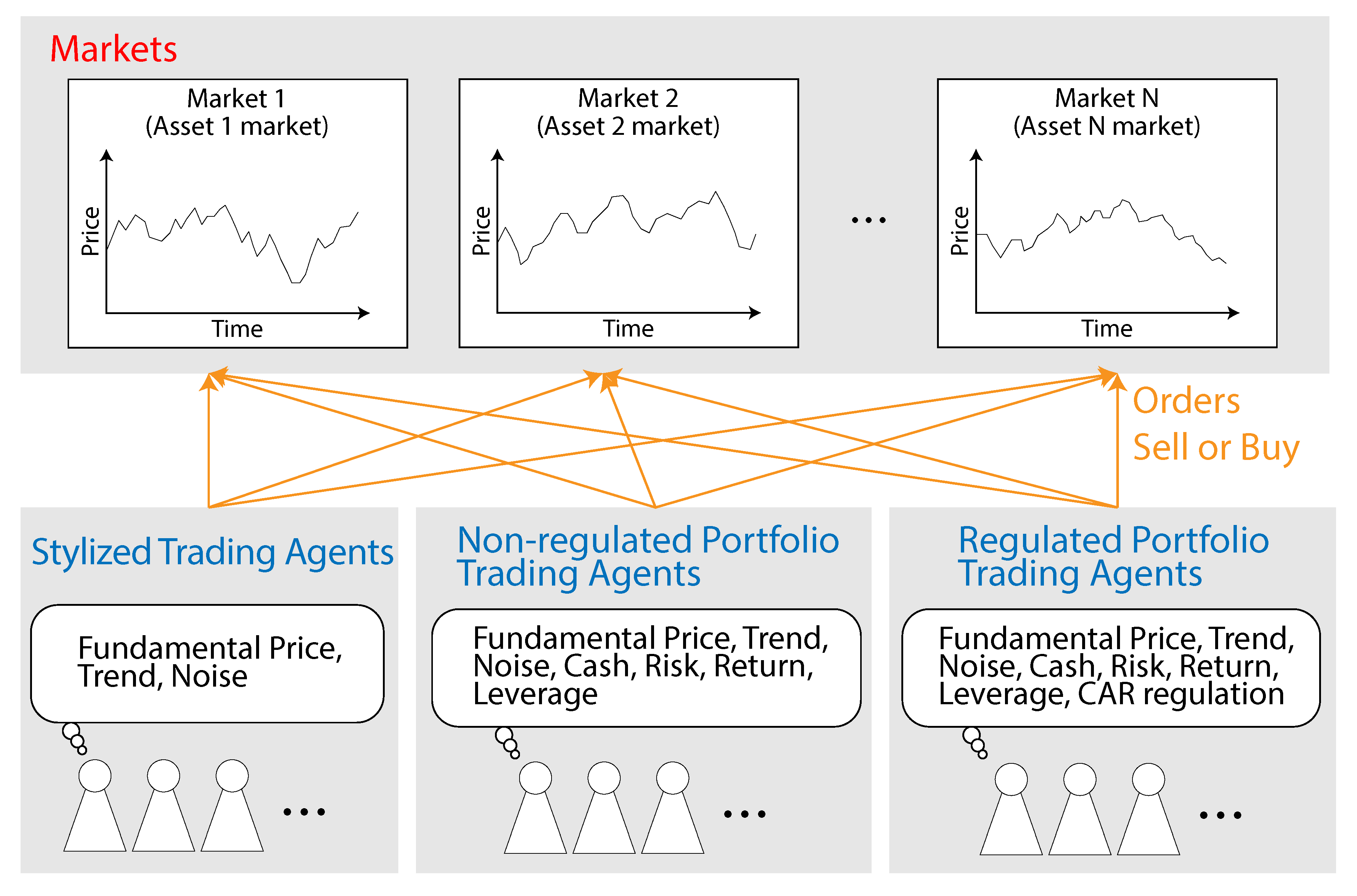
Here, we describe the new multi-asset model of the artificial market. The model contains markets and agents of different types, acting like traders in real financial markets and using their own strategies. The types of agents are as follows.
Each agent can buy or sell any asset in the markets subject to restrictions such as cash, leverage, or CAR regulation (
Figure 1). The markets are based on a multi-asset artificial market of
Torii et al. (
2015). The stylized trading agents are based on a model of
Chiarella and Iori (
2002).
In every step of the simulation, some agents are chosen and place their orders. The number of those agents is the same number as the number of markets. Thus, it is not fixed how many orders are placed or how many orders are contracted in one step.
3.1. Markets
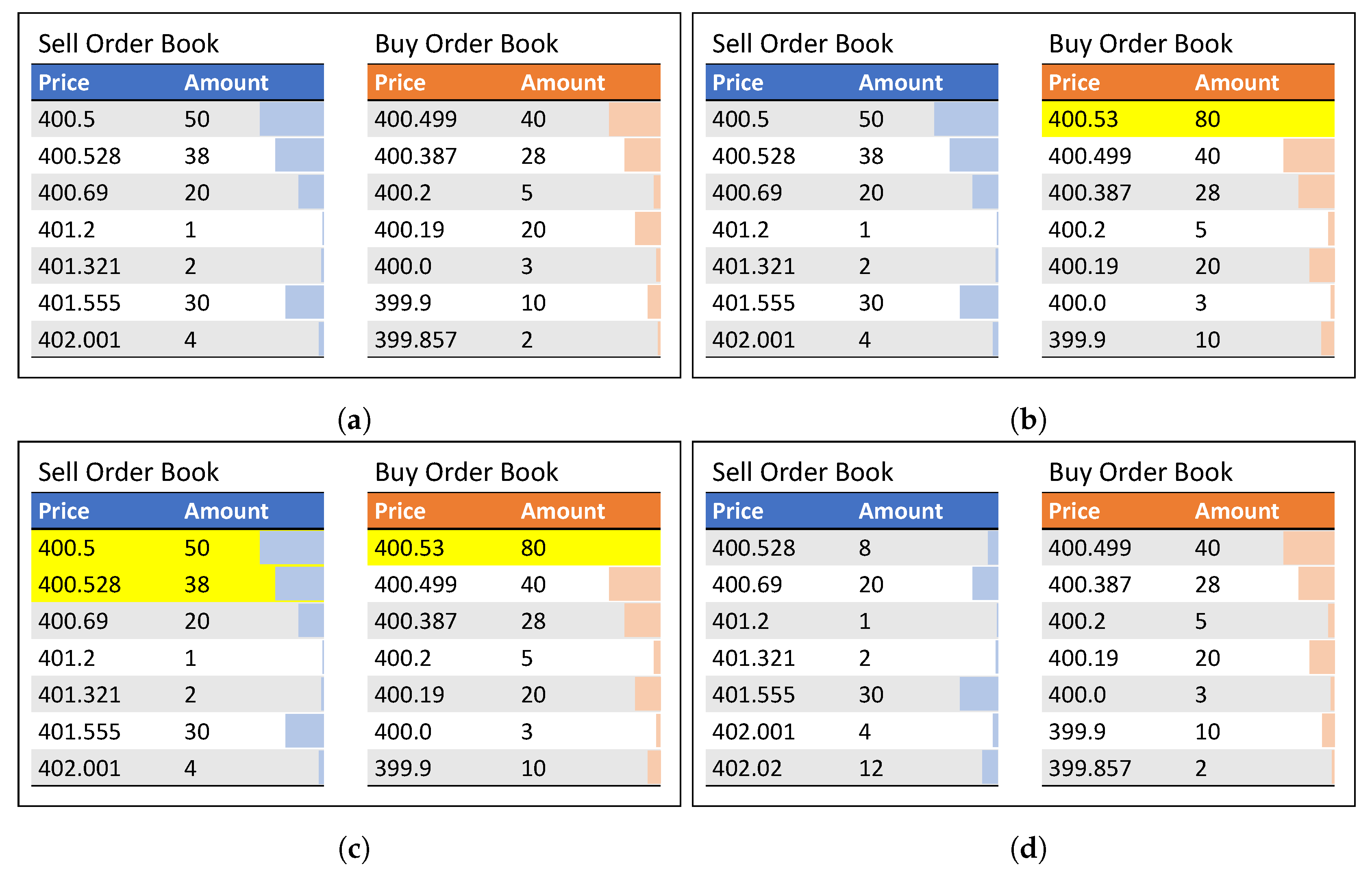
Every asset has a unique market with a continuous double auction mechanism for setting the market price. Any sell or buy order can be placed, and the prices of orders are real numbers (not limited to integers). Examples of order books are shown in
Figure 2. Before inputting a new order, usually, there are also other orders on both sell and buy order books (
Figure 2a). Then, if one agent input 80 buy orders at 400.53, the orders are placed on a buy order book (
Figure 2b). In the case of the order books that appear in
Figure 2, the 80 new buy orders can be contracted with existing sell orders, 50 sell orders at the price of 400.5 and 30 orders in 38 sell orders at the price of 400.528 (
Figure 2c). After contracting, only 8 sell orders in 38 sell orders at the price of 400.528 are still on the sell book, and all contracted orders vanish (
Figure 2d).
Market prices are decided separately for every asset in each market through the continuous double auction mechanism. Transaction fees are ignored.
Every asset has a fundamental price. This price is for agents to decide their own estimated value for each asset, and determined in accordance with multivariate geometric Brownian motion (known as a random walk). In the simulations, the start of the Brownian motion was set at 400.0, and the variance was set at
based on
Torii et al. (
2015).
In addition, we assumed that there was no correlation between any pairs of assets.
3.2. Agents
The three types of agent roughly imitate traders in real markets. Each one has its own trading strategy or trading algorithm, which is explained below. Initially, all agents have 50 assets per market.
3.3. Agents: Stylized Trading Agents
In every step, the stylized trading agents estimate their reasonable price for each asset by using historical data and fundamental prices. They use three types of index, which they calculate by themselves using their own unique parameters.
A stylized trading agent, agent i, decides its reasonable price for asset (market) s at time t, as follows.
Agent
i has three unique weights;
for
F,
for
C, and
for
N (where
). The estimated logarithmic return
is
As described below, , , and were set to exponential distributions with means of 10.0, 1.0, and 10.0.
Fundamental factor , chartist factor , and noise factor for agent i at time t are calculated:
Fundamental factor:
where
is the price at time
t,
is the fundamental price at time
t (given by the geometric Brownian motion as we mentioned above), and
is agent
i’s mean-reversion-time constant (This indicates how long the agent assumes it takes for the price to go back to the fundamental price).
Chartist factor:
where
is agent
i’s time window size, which means how far back into the past the historical data goes that the agent uses.
Noise factor:
which means that
obeys a normal distribution with a zero mean and the variance
.
In the simulations,
was a uniform distribution
,
was a uniform distribution
, and
based on
Torii et al. (
2015).
On the basis of the Equations above, the agent decides its reasonable price
at time
:
Then, on the basis of this price, the agent decides whether to buy or sell one unit share; if , the agent buys one unit of asset s, and if not, the agent sells one unit of asset s at time t.
Stylized trading agents are aimed at making enough orders for contracting. This is because if there were few orders on the markets’ order books, an agent’s order would not be contracted when other portfolio trading agents make orders. Thus, only stylized trading agents are allowed to “sell short” and “margin trade.” Sell short is to place sell orders without holding stock. Margin trade is to place orders without holding enough money.
In addition, stylized trading agents can access and buy or sell any asset in the markets. They make decisions separately, whether they will buy or sell each asset.
3.4. Agents: Non-Regulated Portfolio Trading Agents
Non-regulated portfolio trading agents have a trading strategy based on portfolio optimization.
In the same way as stylized trading agents, non-regulated portfolio trading agents can access all markets and can buy or sell any asset. However, in contrast to stylized trading agents, non-regulated portfolio trading agents choose their position, how many shares of each asset they will buy or sell, inclusively. That is, whether they will buy or sell an asset depends on the other assets, and the decision also depends on the results of the portfolio optimization.
Non-regulated portfolio trading agents optimize their position in each step. is the term in which to keep the current position. This variable is given at random to each agent, following an exponential distribution whose mean and standard deviation are each 150. Thus, the agents take actions only in each step. The actions are as follows.
Cancel orders which have not been contracted yet.
Calculate reasonable values of every asset in the same way as stylized trading agents.
Revise the portfolio with the portfolio optimization algorithm described below.
On the basis of the revised portfolio, make orders for the difference with those of the current portfolio.
Markowitz’s mean-variance approach (
Markowitz 1952) is used in the optimization phase (the third phase above). The expected utility function is defined with a position matrix
, matrix of reasonable values
, and variance-covariance matrix of every asset for the last
steps
.
means the transposed matrix of
A.
The constraints are as follows. The agents have a budget, and they are not allowed to sell short. Thus, all components in are nonnegative. Agents find that fits the constraints and maximizes .
Non-regulated portfolio trading agents have capital and leverage. In the simulations, the capital was 6000 per market and the leverage limit was 10, which means that the budget limit is 60,000 per market. For example, if there are five markets, the budget limit is 300,000.
3.5. Agents: Regulated Portfolio Trading Agents
The CAR regulation in this model uses the Value at Risk (VaR) and regulates agents when the value of assets held by each agent falls.
Markets risk is calculated as
The current total share price does not include cash because cash is meant to be a non-risk property. According to this equation, the more leverage agents take on, the more risk they have to take on as well. The “” part indicates the possible amount of the decrease in asset value using VaR. Because VaR is calculated on a logarithmic scale, it is included as an exponent in this equation.
This calculation involves taking the floor of the upper one-sided confidence interval and uses the root T multiply method (
FFR+ 2008).
is the position matrix of all assets. The holding term of an asset
T is set to 10 steps, and
is the variance-covariance matrix of all assets for the last 250 steps, as described in Basel I and II (
Basle Committee on Banking Supervision 1996b), whose CAR regulation uses historical data for 250 business days and expects a holding term of 10 business days.
When the agents’ portfolio violates the regulation, they revise their portfolios as follows.
Calculate CAR based on the current position (referred to as ).
Calculate the current total share price using and a reasonable value calculated in the same way as stylized trading agents.
Calculate the new budget limit
B.
Under the budget limit
B, re-optimize the portfolio and update
by Markowitz’s mean-variance approach presented in
Section 3.4.
If the portfolio still violates Equation (
12), go to step 1 again. If not,
is the final position, which does not violate the CAR regulation.
3.6. Parameters
All agents have parameters. Some parameters were decided beforehand; others were decided by conducting a parameter search over a number of simulations. The agent parameters decided by parameter search are
Amount of cash per market that each agent holds
: Weight for fundamentalist
: Weight for chartist
: Weight for noise
These parameters are decided by simulating with many parameter sets. In this study, the candidates for the amount of cash were 4000, 6000, 8000, and 12,000, while the candidates for the weights were exponential distributions with means of 1.0, 3.0, 5.0, and 10.0. Then, the target kurtosis of the market price change was set to about 15 for five markets, 1000 stylized trading agents, and 100 non-regulated portfolio trading agents. Kurtosis,
, is defined with the logarithmic return
:
Kurtosis was used in the parameter search because a large kurtosis is a feature of “fat-tailed” distributions and a stylized fact characterizing real markets (
Cont 2001). Here, events that rarely occur in accordance with a normal (Gaussian) distribution occur more often when they follow a fat-tailed distribution. Because
for the normal (Gaussian) distribution, it is a good index for indicating a fat tail.
According to
Table 1 and
Table 2, the possible kurtosis seems to be under 20. The test with five markets, 1000 stylized trading agents, and 100 non-regulated portfolio trading agents showed price changes with comparatively higher kurtosis than those of other simulations in this study. So, we assumed the target kurtosis to be about 15.
In addition, we checked for “absence of autocorrelations” and “volatility clustering”, which are two of Cont’s stylized facts (
Cont 2001).
The parameter search yielded the following results.
Amount of cash per market that each agent holds
: Weight for fundamentalist → exponential distribution with mean 10.0
: Weight for chartist → exponential distribution with mean 1.0
: Weight for noise → exponential distribution with mean 10.0
4. Experiments
We designed two different experiments: one for assessing the effect of portfolio trading agents, the other for checking the effect of the CAR regulation.
Before explaining each experiment, we should explain the evaluation index. The index evaluates how many steps the market price drops abnormally. We define “abnormal” as:
In this equation,
means the market price, and
means the fundamental price. Moreover,
is defined as the number of steps in which Equation (
14) is satisfied.
The common settings for the simulations were as follows.
Pre-running length: 30,000 steps
Simulation length: 60,000 steps
Number of trials: 100 times per parameter set
4.1. Experiments for Assessing Effects of Portfolio Trading Agents
First, using only stylized trading agents and non-regulated portfolio trading agents, as listed below, we experimented on the effect of portfolio trading agents.
Stylized trading agents: 1000 agents (fixed)
Non-regulated portfolio trading agents: agents
Number of markets (number of assets): markets (assets)
4.2. Experiments for Assessing Effects of the CAR Regulation
Second, we included regulated portfolio trading agents. Here, the total number of non-regulated portfolio trading agents and regulated portfolio trading agents were fixed to 100 agents. We experimented by changing the ratio of non-regulated portfolio trading agents and regulated portfolio trading agents.
Stylized trading agents: 1000 agents (fixed)
Non-regulated portfolio trading agents: agents
Regulated portfolio trading agents: agents
Number of markets (number of assets): markets (assets)
5. Results & Discussion
5.1. Stylized Fact Checks
Before we present the results of each type of experiment we mentioned above, we show the results for checking whether stylized facts are also appearing in our simulation. This process is essential to ensure that our simulations are not unrelated ones to the actual market. As stylized facts to check our simulation, we employed the absence of autocorrelations, heavy tails (fat tails), and volatility clustering. These stylized facts were listed on
Cont (
2001) and
Dacorogna et al. (
2001). To ensure our simulation works well, we checked the facts in all parameters sets in this study by checking plots. However, here we show the results from the simulation with 1000 stylized trading agents, 50 non-regulated portfolio agents, 50 regulated portfolio agents, and 5 markets.
In the following, we check these stylized facts each by each.
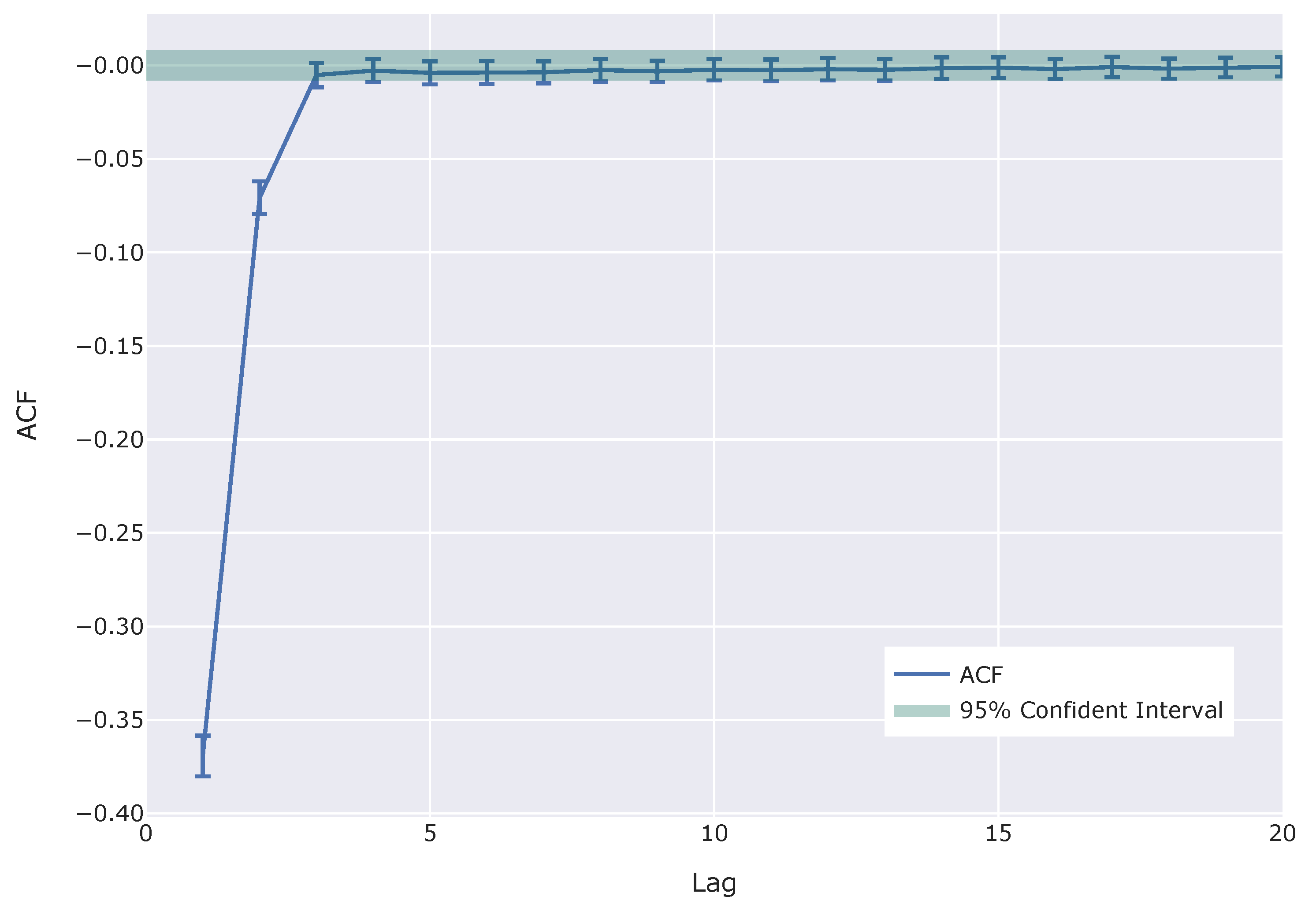
At first, we checked the absence of autocorrelation. Here, we calculate the autocorrelation of logarithm returns.
Figure 3 shows autocorrelation function (ACF) for logarithm returns. This result clearly shows the absence of autocorrelation. It is because the autocorrelation is statistically significant only for very small lags. This result agrees nicely with the fact shown in
Cont (
2001) and
Dacorogna et al. (
2001).
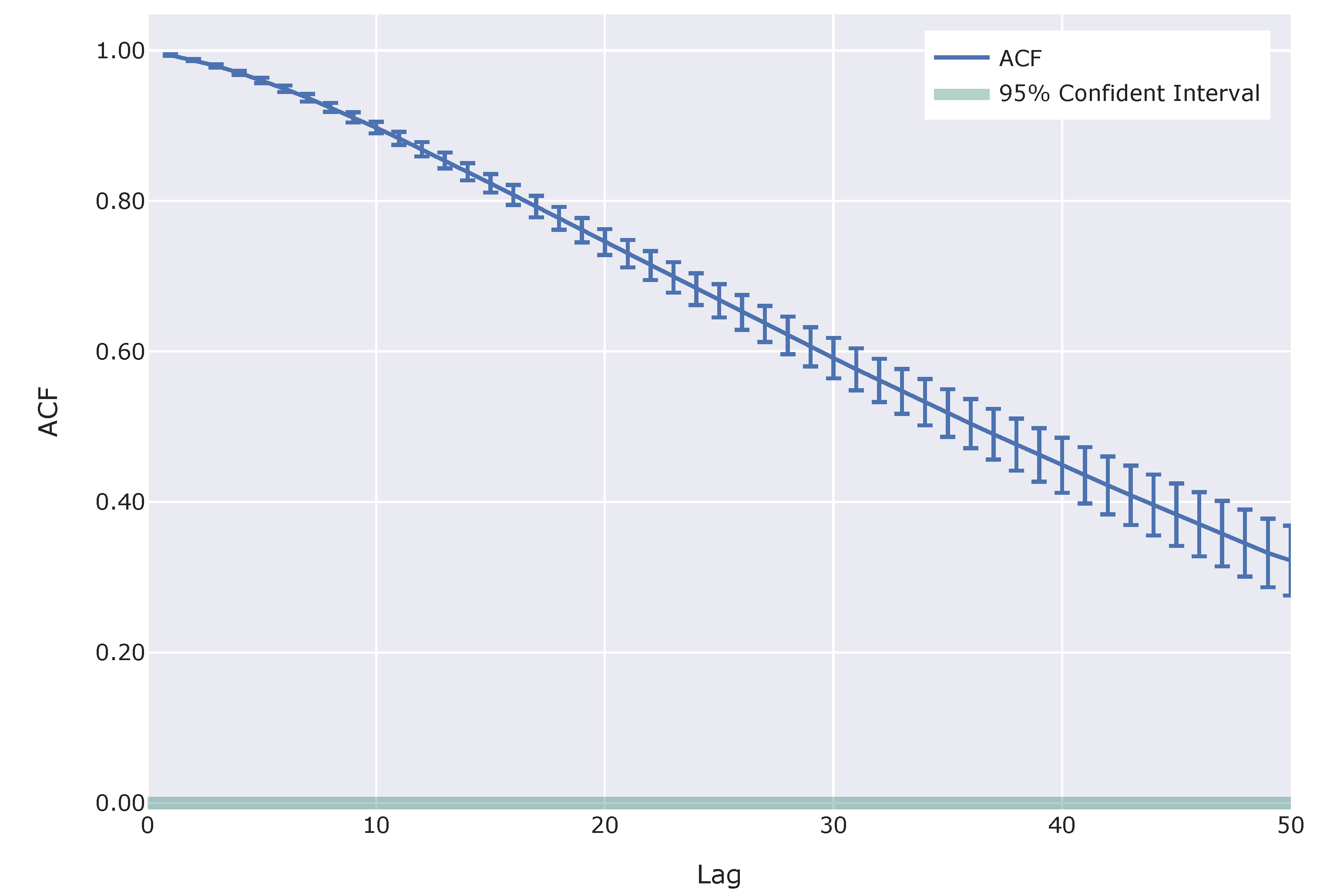
Next, we checked the volatility clustering. Here, we tested the autocorrelations of 50-step standard deviations of logarithm returns.
Figure 4 shows autocorrelation function (ACF) for 50-step standard deviations of logarithm returns of logarithm returns. This also clearly shows the volatility clustering. The autocorrelation function is statistically significant. It means that there are autocorrelations for standard deviation, i.e., volatility. This result also agrees with the stylized fact shown in
Cont (
2001) and
Dacorogna et al. (
2001).
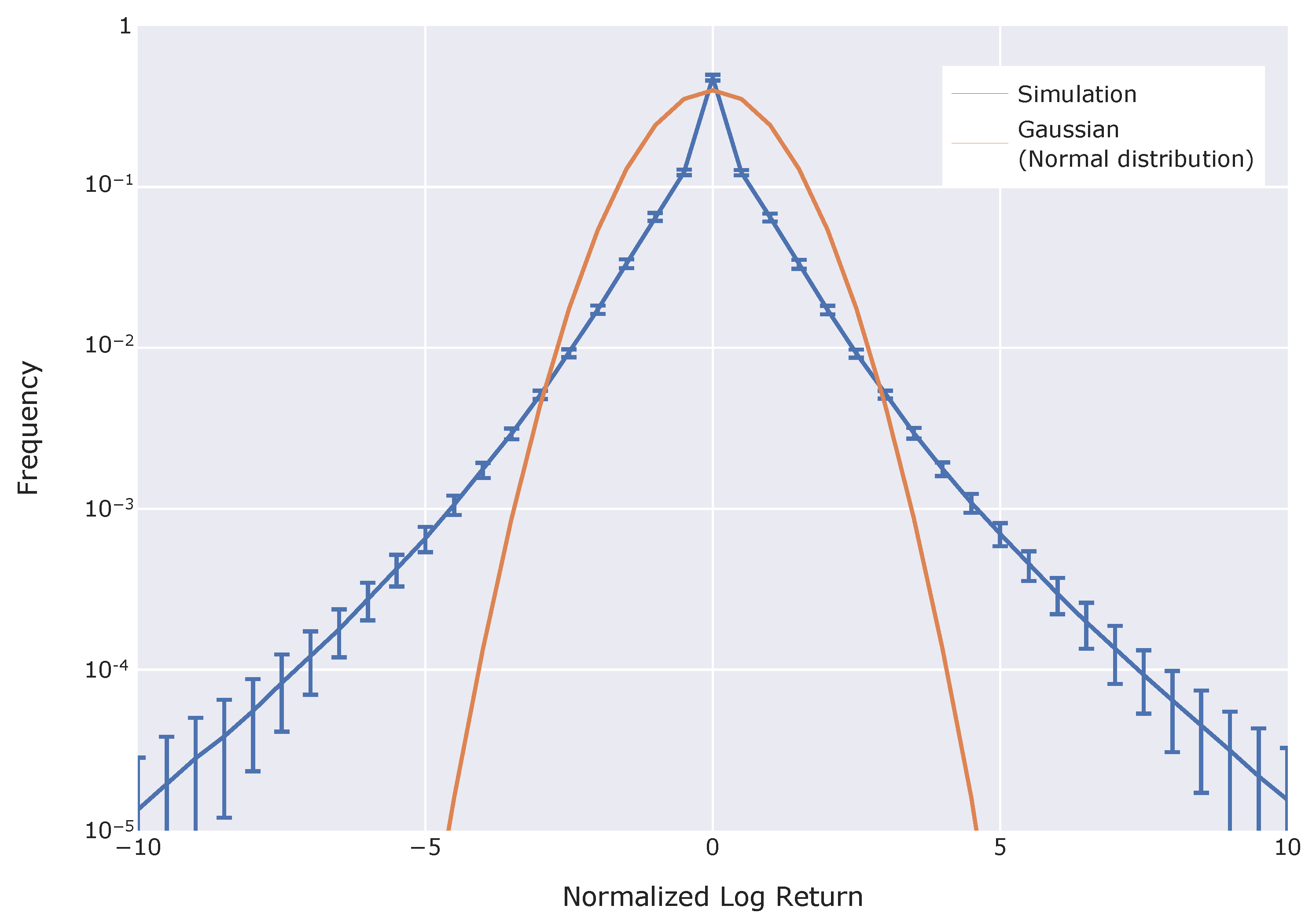
At last, we confirmed the heavy tail (fat tail) in return distributions. To investigate the existence of heavy tails, we processed the time-series market prices in simulations. At first, we calculated logarithm returns from market prices. Then, we normalized these returns in each market in each simulation. Moreover, based on these normalized returns, we made frequency distributions. According to the frequency distributions, we made
Figure 5. In addition, for comparisons, we also plot the Gaussian (normal) distribution on
Figure 5.
According to
Figure 5, the simulation results have a significant heavy tail (fat tail). This result also shows that our simulations can reproduce one of the stylized facts.
According to the results we showed above, we can assume that our simulations can reproduce some stylized facts in real markets. This may indicate that our simulations are reliable at a certain level.
As future work, we should further ensure the reliability of our simulations. Of course, it is almost impossible to prove that simulations are entirely reliable. However, we should keep trying to ensure reliability by some methods including checking stylized facts.
5.2. Effects of Portfolio Trading Agents
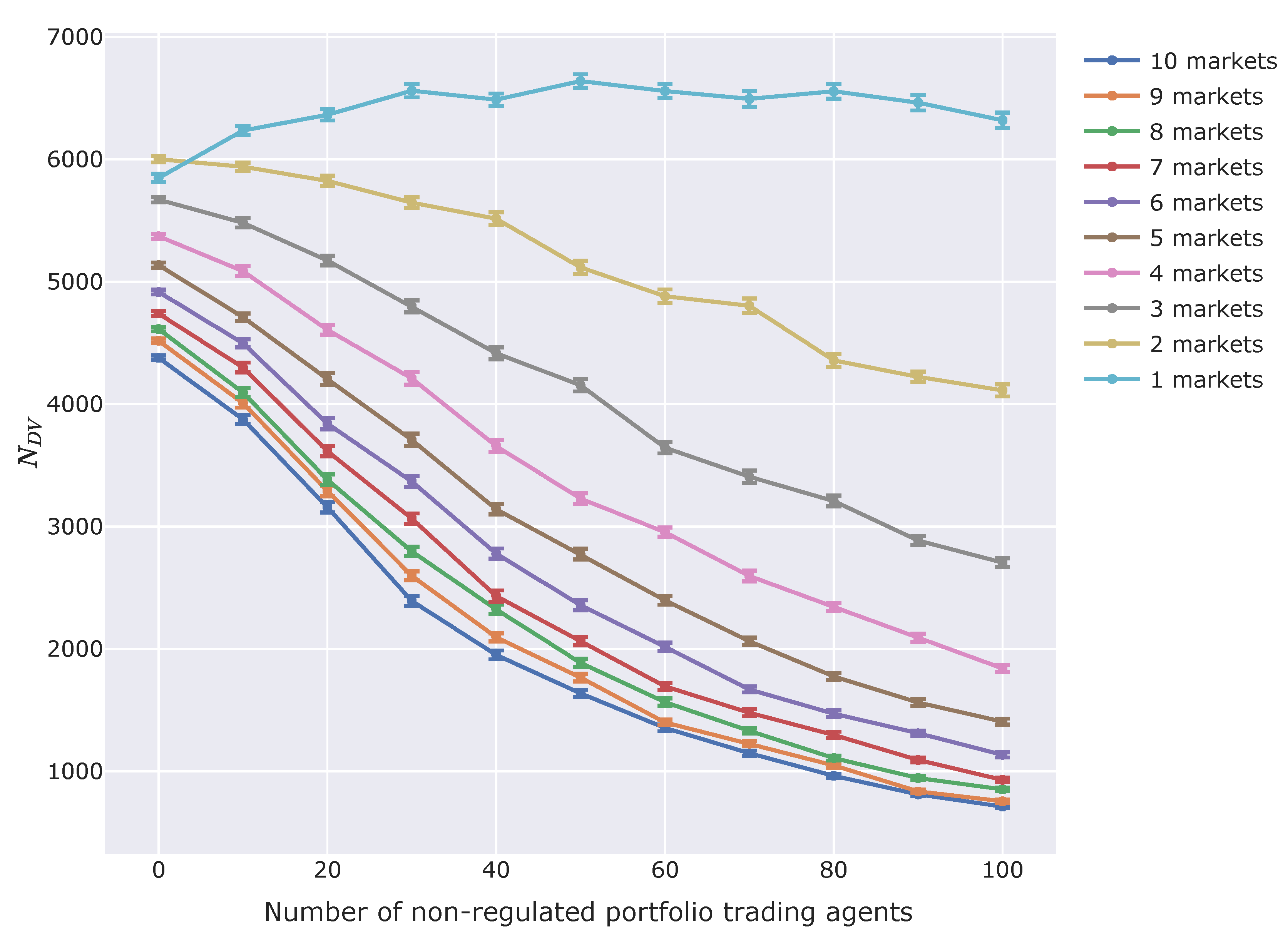
Figure 6 shows the results of the experiments assessing the effect of portfolio trading agents.
According to
Figure 6, the more non-regulated portfolio trading agents there are in the markets, the fewer steps there are whose market price goes below
times the fundamental price. This means non-regulated portfolio trading agents stabilize markets when there are multiple markets (assets). However, rightly, there is not the tendency when there is only one market (asset).
Ordinarily, portfolio optimization is thought to stabilize only individual trading returns. However, these results show that portfolio optimization can also stabilize whole markets.
In our opinion, because portfolio optimization can find market equilibria points, it can improve the efficiency of markets. In short, portfolio optimization might help to find the correct value for each asset, and it has a stabilizing effect on markets.
In addition,
Figure 6 shows that the more assets there are in portfolios, the more stable that markets become. Additionally, in the case of 5–10 markets, the stabilizing effect saturates. On the other hand, when there is only one market (assets), and agents cannot take portfolio optimization, the stabilizing effect does not appear.
These results also suggest that the number of portfolio trading agents is in the appropriate range to examine these effects. It is because the figure clearly shows changes in .
5.3. Effects of CAR Regulation
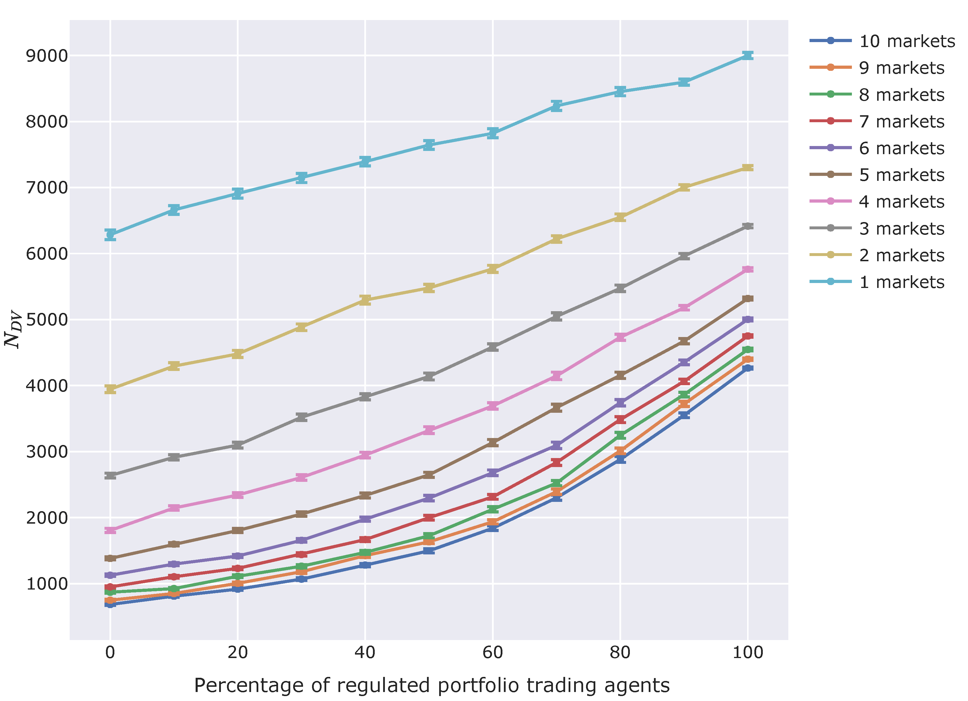
Figure 7 shows the results of the experiments assessing the effect of CAR regulation.
The far left of
Figure 7 shows
in the case that the percentage of regulated portfolio trading agents is 0%. The results here are under the same condition as in the case that the number of portfolio trading agents is 100 in
Figure 6. Precisely, the results are slightly different from those in
Figure 6 because we performed experiments as consecutive different experiments from the experiments for
Figure 6. However, the results are almost the same.
According to this graph, regulated portfolio trading agents make larger, which means CAR regulation causes more and more price shocks.
Moreover, when the percentage of portfolio trading agents regulated by Basel is 100%, the difference in between the instances of one market and ten markets is smaller than when the percentage is 0%. It suggested that CAR regulation can suppress the stabilizing effect of portfolio trading agents.
These results show that CAR regulation may destabilize markets even if there are multiple markets (assets) and portfolio trading agents have great stabilizing effects on markets.
Let us consider why this happens. CAR regulation would be invoked when market prices fall and risks of holding assets increase; this means that agents would have to sell their assets. In turn, the regulation would have more and more impact on other agents, i.e., the regulation causes assets sellings and the asset sellings trigger other’s regulations. Thus, under these conditions, selling would induce more selling and lead to significant price shocks.
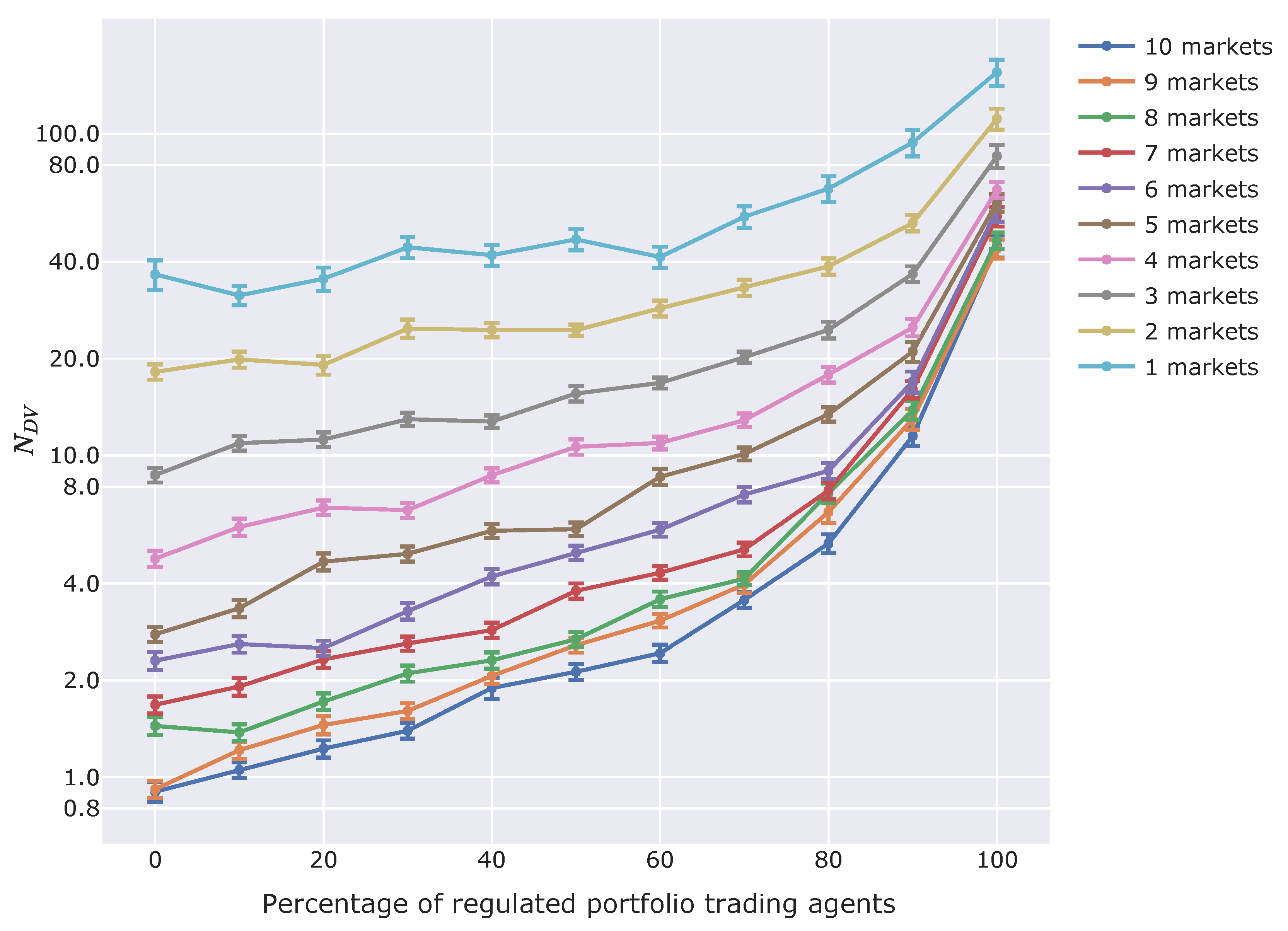
To ensure the results, we also checked the more significant shocks. Thus, we modified the threshold of the definition of Equation (14) as:
Then, we made a plot of
in the same manner as in
Figure 7. The result is shown in
Figure 8.
Also, in
Figure 8, there is the same tendency as in
Figure 7. Even if the threshold is
times the fundamental price, there are some steps in which the market price is below the threshold. About
of fundamental prices are quite significant price shocks.
Moreover, the tendency, i.e., more regulated portfolio trading agent on markets cause more price shocks, is more significant when there are fewer numbers of markets. When there are ten markets and no regulated portfolio trading agent, the significant price shocks defined in Equation (
15) happened in only about 1 step in 60,000 steps on average. However, when all the portfolio trading agents are regulated, it happened more than 40 steps, even if there are ten markets.
Now, let us look for other effects of CAR regulation by examining
Figure 9 and
Figure 10.
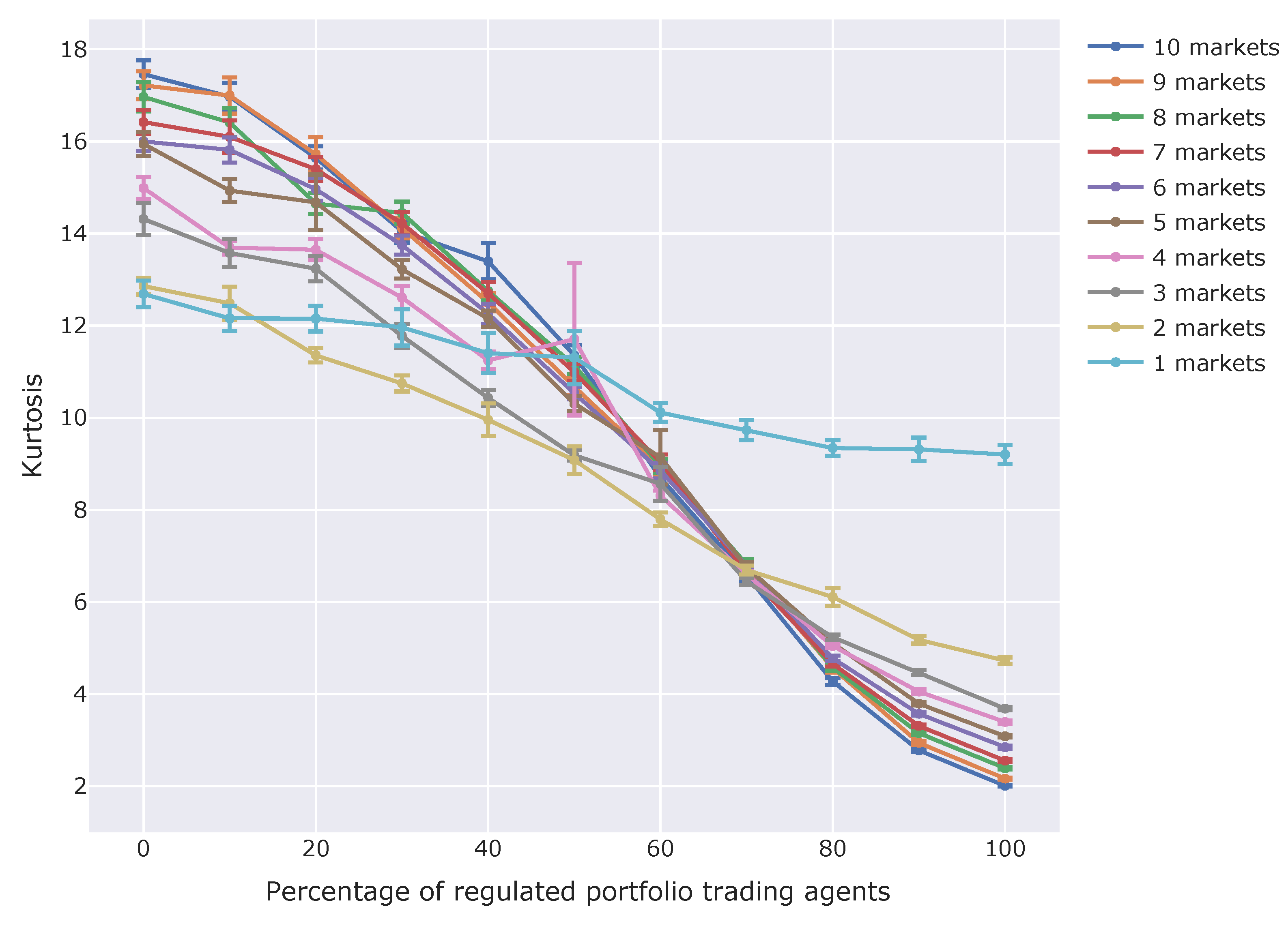
Figure 9 shows the kurtosis of price changes. The definition of kurtosis is the same as in Equation (
13).
According to this figure, having more regulated portfolio trading agents decreases kurtosis. This suggests that CAR regulation eliminates the fat-tail tendency from markets.
The results depicted in the and kurtosis graphs suggest the following hypothesis: CAR regulation depresses prices and decreases the chances of market prices rising. We have already confirmed the fact that CAR regulation causes more price shocks and eliminates the fat-tail tendency. Thus, we suspect that the overall decline in prices had led to a low fat-tail even when the price shocks happened more frequently. Moreover, we also suspect that CAR regulation causes decreases the chances of market prices rising. The reason we assumed this is that a rising market price indicates that there is more chance of the price decreasing. In addition, agents sell assets during sudden market price rises, because the chance of a price shock also increases in the CAR regulatory framework.
Thus, CAR regulation may depress whole markets.
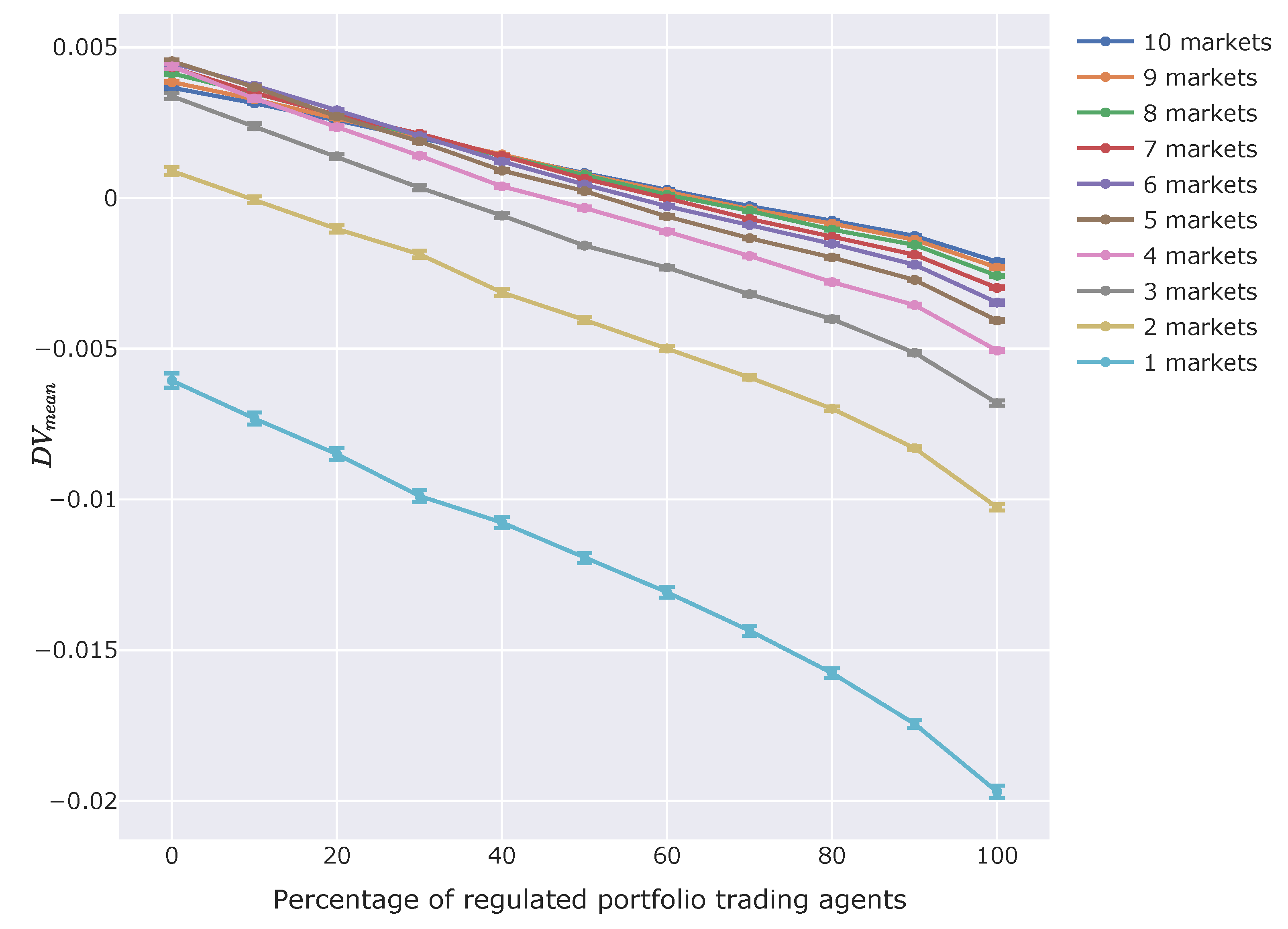
Figure 10 shows the changes in mean
.
is defined in Equation (14); it is the ratio of the market price to the fundamental price.
Figure 10 shows that a greater number of regulated portfolio trading agents depress the mean of
. It clearly shows that CAR regulation depresses whole markets.
In addition, we also checked the qualitative price fluctuations.
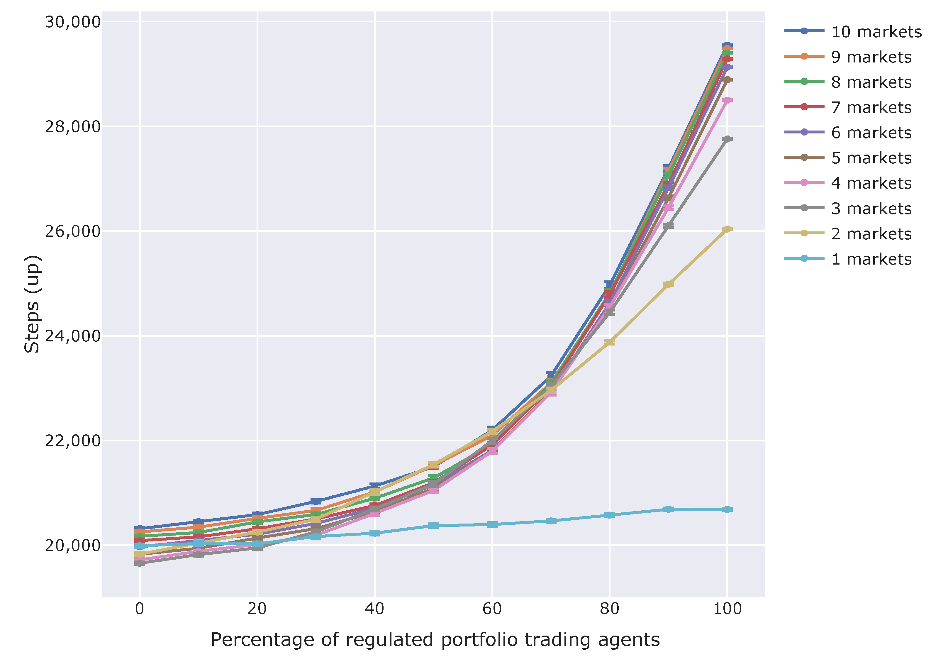
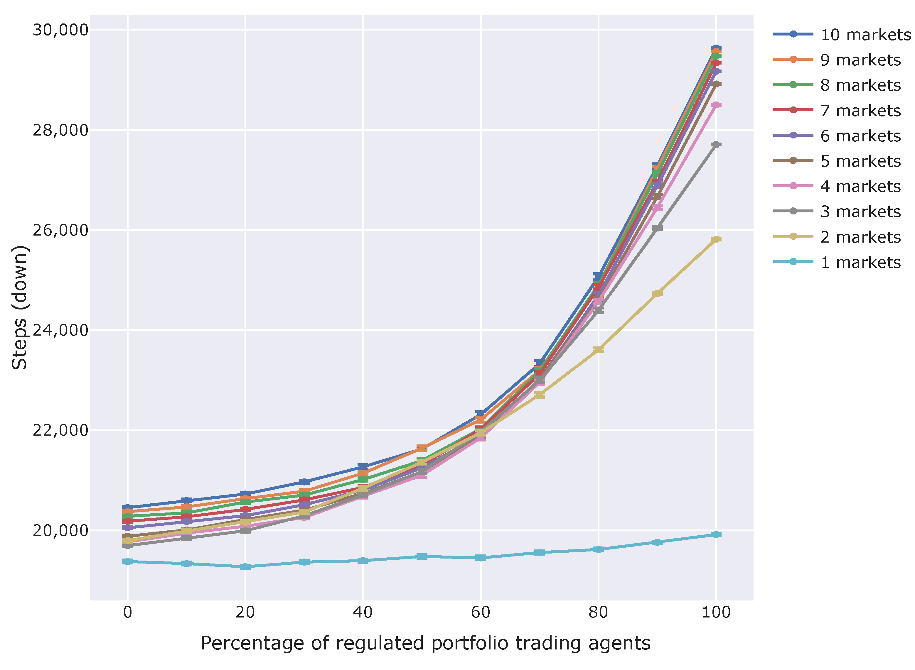
Figure 11 and
Figure 12 show the average steps in which market prices go up or down.
According to the results, the more portfolio trading agents there are on markets, the more the market prices fluctuate. In both
Figure 11 and
Figure 12, increasing the percentage of regulated portfolio trading agents cause more steps in which the market prices went up or down. These results show that there are fewer steps in which the market prices stayed the same when there are more regulated agents. This means markets fluctuate more due to CAR regulation. Moreover, this tendency is supposed to not come from price shocks confirmed above. It is because, if this effect came from the price shocks, only the increase in the steps in which the market prices went down would be shown.
5.4. Summary of Results and its Discussion
The results obtained by the simulation and their interpretation are summarized in
Table 3. In
Table 3, the descriptions are simplified and become easy to understand. “Less Regulated” means the case when there are fewer numbers of regulated portfolio trading agents such as 0%. On the other hand, “More Regulated” means the case when there are bigger numbers of regulated portfolio trading agents such as 100%. The other descriptions are also simplified and relative.
As we mentioned before, price shocks happened more with more regulated agents. It is also assumed to enhance the fat tail of the lower side.
Moreover, kurtosis was also low when there are more regulated agents. It means the fat tail of price change (return) distribution was diminished.
Gathering the facts above, we can assume that the regulation also diminished the fat tail of the upper side of price change (return) distribution. This means that CAR regulation can depress the chance of price rising.
Since we also confirmed a decrease in the mean of market prices, the depressing effects of CAR regulation are supposed to be various.
Moreover, we also confirmed the additional fluctuation due to the regulation through the change in the frequency of price moving (up and down).
In summary, we suppose that four dynamics due to CAR regulation are at play:
5.5. Future Work
In this subsection, we discuss future work.
At first, as future work, the negative effect of CAR regulation shown in this paper should be confirmed empirically. Simulation is helpful to test a hypothetical situation or to help us understand what happened. However, the combination of simulation and empirical research on CAR regulation make our argument more solid.
Moreover, we examine other ways of calculating risks. Now, we employed VaR (Value at Risk). However, there are other ways to calculate risks, such as the expected shortfall.
In terms of CAR regulation, we should consider how to balance both positive and negative aspects of CAR regulation. In this paper, we showed and emphasized only the negative aspect. However, originally, CAR regulation and Basel regulatory framework were designed to prevent a chain bankruptcy in bank networks. So, the impact of regulation on financial markets is secondary. Thus, we should not focus only on the negative effect on financial markets but also consider it as a whole, including bank networks.
6. Conclusions
In this paper, we examined the effect of CAR regulation in agent-based simulations. By using agents who buy or sell at reasonable prices—agents whose strategy is portfolio optimization, and agents whose strategy is portfolio optimization under the regulation in artificial markets—we simulated two scenarios. The results lead us to the following conclusions:
Adopting portfolio optimization as each agent’s strategy stabilizes markets.
The existence of a CAR regulation destabilizes markets.
CAR regulation can cause significant price shocks.
CAR regulation may suppress price increases.
CAR regulation pushes down market prices.
CAR regulation fluctuates market price.
Thus, we conclude that CAR regulation has negative effects on markets widely. Although it might be adequate to prevent systemic risks and chain bankruptcy, CAR regulation can have negative effects, at least, on assets markets. Moreover, if significant price shocks happen because of CAR regulation, there is a possibility that bankruptcies are caused because of the price shocks. Thus, we should balance the positive and negative aspects of CAR regulation.
In this study, we contribute to assessing the impact of CAR regulation via simulations. Our simulation study is beneficial to asses the situation that never happened yet. Usually, empirical studies are only able to assess the impact on the realized situation.
Regarding future work, our finding that CAR regulation can suppress price increases is a new finding that should be the subject of verification empirically. Moreover, we should examine other ways to calculate risk, e.g., by using the expected shortfall in the latest CAR regulation, instead of the VaR used in this study.
