Article

Improving Many Volatility Forecasts Using Cross-Sectional Volatility Clusters

Department of Economics and Statistics, University of Salerno, Via Giovanni Paolo II, 132, 84084 Fisciano (SA), Italy
*
Author to whom correspondence should be addressed.
J. Risk Financial Manag. 2020, 13(4), 64; https://doi.org/10.3390/jrfm13040064
Submission received: 7 February 2020 / Revised: 21 March 2020 / Accepted: 22 March 2020 / Published: 29 March 2020
(This article belongs to the Special Issue Financial Time Series: Methods & Models)

Abstract

:
The inhomogeneity of the cross-sectional distribution of realized assets’ volatility is explored and used to build a novel class of GARCH (Generalized Autoregressive Conditional Heteroskedasticity) models. The inhomogeneity of the cross-sectional distribution of realized volatility is captured by a finite Gaussian mixture model plus a uniform component that represents abnormal variations in volatility. Based on the cross-sectional mixture model, at each time point, memberships of assets to risk groups are retrieved via maximum likelihood estimation, as well as the probability that an asset belongs to a specific risk group. The latter is profitably used for specifying a state-dependent model for volatility forecasting. We propose novel GARCH-type specifications the parameters of which act “clusterwise” conditional on past information on the volatility clusters. The empirical performance of the proposed models is assessed by means of an application to a panel of U.S. stocks traded on the NYSE. An extensive forecasting experiment shows that, when the main goal is to improve overall many univariate volatility forecasts, the method proposed in this paper has some advantages over the state-of-the-arts methods.

1. Introduction

A well known stylized fact in financial econometrics states that the dynamics of conditional volatility are state dependent since they are affected by the (latent) long-run level of volatility itself. This issue has motivated a variety of time varying extensions of the standard GARCH class of models including latent state regime-switching models (Gallo and Otranto 2018; Hamilton and Susmel 1994; Marcucci 2005), observation-driven regime switching models (Bauwens and Storti 2009, WGARCH), Generalized Autoregressive Score (Creal et al. 2013, GAS) models, Component GARCH models (Engle et al. 2013, GARCH-MIDAS), (Engle and Rangel 2008, Spline-GARCH). All these models, directly or indirectly, relate the conditional variance dynamics to its long-run level.
At the same time, in recent years there has been a growing interest in modeling the volatility of large dimensional portfolios with a particular interest in the dynamic inter-dependencies among several assets (Barigozzi et al. 2014; Engle et al. 2019). However, modeling dynamic interdependencies among several assets would in principle require the estimation of an unrealistic huge number of parameters compared with the available data dimensions. Model’s parsimony is achieved introducing severe constraints on the dependence structure of the data (see Pakel et al. 2011). In this respect, Bauwens and Rombouts (2007) showed evidence in favor of the hypothesis that there exist cluster-wise dependence structures in the distribution of financial returns.
In this paper, we propose a novel approach to modelling volatility dynamics for large panels of stocks. In particular, we exploit the cluster structure of returns at cross-sectional level to build GARCH-type models where the volatility of each assets depends on the past information about the cluster structure of the entire market. Although this does not provide a multivariate volatility model for the entire market, the proposed strategy allows to build univariate models that parsimoniously use past information on the entire market. In each time period, a robust model-based clustering method identifies G volatility groups based on realized volatility data. The model-based methodology allows to assign assets to volatility clusters based on a mixture probability model assumed for the cross-sectional distribution of the realized volatility. Each volatility cluster is represented by a Gaussian distribution, and the robustness of the assignment is ensured via the addition of uniform mixture component to capture abnormal variations in realized volatility. In fact, these observed abnormal realized volatility typically have an extremely scattered behavior not consistent with the main clusters referred as “regular clusters” in this work. The robust model-based clustering algorithm is based on the contribution of Banfield and Raftery (1993) and Coretto and Hennig (2011). The novelty here is that the aforementioned contributions are extended including constraints that ensures the desired separation between “regular” clusters, and (outlying) clusters representing abnormal volatility. Then, for a given asset, its volatility is modeled via a GARCH-type model where parameters depend on the discovered group-structure in previous periods. The proposed modelling approach is also related to the stream of literature on state-dependent volatility modelling given that, for any specific asset, the information on cluster membership can be seen as a synthetic measure of the volatility level of the asset, with respect to the cross-sectional distribution of volatility at a given time point. The underlying idea is that the identified clusters can be related to factors characterized by different relative volatility levels. Each of these factors is then allowed, but not constrained, to have different dynamic properties. Assets can migrate from one group to another, so that we obtain a form of time-varying state-dependent conditional variance process determined on the basis of its volatility level relative to the market cross-sectional level. The latter introduces a novelty in the literature where the state-dependent nature of the volatility process has been treated in terms of absolute volatility levels (see for example, Bauwens and Storti 2009, and references therein).
The paper is organized as follows: in Section 2 we introduce the proposed GARCH-type specification and the supporting clustering method while the related estimation procedure is discussed in Section 3. In Section 4 we present the results of an application using data on a portfolio of stocks traded in the NYSE and, finally, in Section 5 we state some final remarks.

2. A Garch-Type Specifications Incorporating Cross-Sectional Volatility Clusters

2.1. The CW-GARCH Specification

Consider a market with s = 1 , 2 , , S assets traded at times t = 1 , 2 , , T . At each time period t an asset s belongs to a volatility group j, where j = 1 , 2 , , G . Therefore it is assumed that the cross-sectional distribution of assets’ volatility exhibits a group structure. A volatility cluster is understood as a group of assets that, at time t, have an “homogeneous” distribution in terms of volatility. The homogeneity concept underlying the cluster model is explained in the subsequent Section 2.2. Volatility clusters are groups of assets with similar risk, therefore referred as “risk groups”. We assume that there are G fixed volatility clusters, where G is not known to the researcher. Each asset s can migrate from one cluster to another, but the number of clusters G is assumed to be fixed for the entire time horizon. The class labels are arranged so that they induce a natural ordering in terms of the riskiness of their assets. That is, for any j a < j b , group j b is riskier than group j a . This ordering is not in generally necessary from the technical viewpoint since any asset is allowed to migrate from any group to any other group, however it is adopted to identify the group labels in terms of low-vs-high volatility.
Let I { A } be the indicator function at the set A, let I t 1 be the information set at time t 1 , and let E [ · | I t 1 ] denote the expectation conditional on I t 1 . Define the indicator variables
D t , s , j = I { asset s group j at time t } ,
and assume that E [ D t , s , j | I t 1 ] = π t , j [ 0 , 1 ] . That is, at time t the j-th group is expected to contain a proportion of π t , j assets. In other words π t , j captures the expected size of the j-th cluster at time t. The vector g t , s = ( D t , s , 1 , D t , s , 2 , , D t , s , G ) is a complete description of the class memberships of the s-th asset at time t. The elements of g t , s are called “hard memberships”, because these link each asset to a unique group inducing a partition at each t.
Let r t , s be the return of the asset s at time t. Let { z t , s } be a sequence of random shocks where z t , s IID ( 0 , 1 ) . Consider the following returns’ generating process
r t , s = μ s + σ t , s z t , s σ t , s 2 = ω s + α s ( r t 1 , s μ ) 2 + β s σ t 1 , s 2 g t 1 , s
where ω s , α s and β s are G-dimensional model parameter vectors. In particular ω s = ω s , 1 ω s , G > 0 , α s = α s , 1 α s , G 0 , β s = β s , 1 β s , G 0 . The clustering information about the cross-sectional volatility enters the model for r t , s via g t 1 .To see the connection with the classical GARCH(1,1) model (Bollerslev 1986), note that
σ t , s 2 = ω s , j + α s , j ( r t 1 , s μ ) 2 + β s , j σ t 1 , s 2 if asset s group j , 0 otherwise .
Therefore, conditional on the groups’ memberships at time t 1 , the model (1) specifies a GARCH(1,1) dynamic structure for all those assets within a given group j. Based on this, model (1) is referred as the “Clusterwise GARCH” (CW-GARCH) model. Within the j-th cluster, the model parameters ω s , j , α s , j and β s , j can be interpreted as usual as the intercept, shock reaction and volatility decay coefficients of the j-latent component. Therefore, we refer to ( ω s , j , α s , j , β s , j ) as the “within-group” GARCH(1,1) coefficients. The advantage of model (1) is that it models the conditional variance dynamic in terms of an ordinal state variable so that the switch between G different regimes is contingent to the overall market behavior. Volatility clusters are arranged in increasing order of risk from j = 1 to j = G , and in two different time periods t 1 and t 2 an asset s may belong to the same risk group, i.e., g t 1 , s = g t 2 , s , leading to the same GARCH regime although its volatility may have changed dramatically because the overall market volatility changed dramatically. The state variable g t 1 , s transforms a cardinal notion, i.e., volatility, into an ordinal notion induced by the memberships to ordered risk groups.
In order to see how the cluster dynamic interacts with the GARCH-type coefficients, define
ω t , s = ω s g t 1 , s = j = 1 G ω s , j D t 1 , s , j , α t , s = α s g t 1 , s = j = 1 G α s , j D t 1 , s , j , β t , s = β s g t 1 , s = j = 1 G β s , j D t 1 , s , j .
The variance dynamic equation in (1) can now be rewritten as
σ t , s 2 = ω t , s + α t , s ( r t 1 , s μ ) 2 + β t , s σ t 1 , s 2 .
Equation (2) resembles a GARCH(1,1) specification with time-varying coefficients obtained by weighting the within-groups classical GARCH(1,1) parameters by the class membership state variables. Although model (2) leads to a convenient interpretation of the model, its formulation is not consistent with a model with dynamic parameters. In fact, the three model parameter vectors ω s , α s , β s do not depend on t, and the dynamic of ω t , s , α t , s , β t , s is driven by the state variables { D t 1 , s , j } .
From (2) it can be seen that the dynamic of σ t , s 2 changes discontinuously because of the transition of an asset from a risk group to another. We introduce an alternative formulation of the model where the dynamic of σ t , s 2 is smoothed by replacing the hard membership state variables { D t 1 , s , j } with a smooth version. There are situations where the membership of an asset is not totally clear (e.g., assets on the border of the transition between two risk groups), in this situation one may desire to smooth the transition between groups. Instead of assigning an asset to a risk group, one can attach a measure of the strength of the membership. In the classification literature these are called “soft labels” or “smooth memberships” (see Hennig et al. 2016). There are various possibilities for defining a smooth assignment. The following choice will be motivated in Section 2.2. Define
τ t , s , j = E [ D t , s , j | I t ] = Pr { D t , s , j = 1 | I t } ,
now τ t , s , j [ 0 , 1 ] , and j = 1 G τ t 1 , s , j = 1 for all t = 1 , 2 , . The quantity τ t , s , j gives the strength at which the asset s is associated to the j-th cluster at time t based on the information at time t. Define the vector τ t , s = ( τ t , s , 1 , τ t , s , 2 , , τ t , s , G ) . We propose the following alternative version of model (1) where the variance dynamic equation is replaced with the following σ ˜ 2 process
r t , s = μ s + σ ˜ t , s z t , s σ ˜ t , s 2 = ω s + α s ( r t 1 , s μ ) 2 + β s σ t 1 , s 2 τ t 1 , s .
We call (4) the “Smooth CW-GARCH” (sCW-GARCH) model. For the sCW-GARCH the variance process can be written as a weighted sum of GARCH(1,1) models
σ ˜ t , s 2 = j = 1 G τ t 1 , j , s ω s , j + α s , j ( r t 1 , s μ ) 2 + β s , s σ t 1 , s 2 .
As before, write the previous equation in terms of time varying GARCH components as follows
σ ˜ t , s 2 = ω ˜ t , s + α ˜ t , s ( r t 1 , s μ ) 2 + β ˜ t , s σ t 1 , s 2 ,
where
ω ˜ t , s = ω s τ t 1 , s = j = 1 G ω s , j τ t 1 , s , j , α ˜ t , s = α s τ t 1 , s = j = 1 G α s , j τ t 1 , s , j , β ˜ t , s = β s τ t 1 , s = j = 1 G β s , j τ t 1 , s , j .
From the latter it can be easily seen that the sort of time varying GARCH(1,1) components of the sCW-GARCH change smoothly as assets migrate from one risk group to another. In this case, the formulation above gives also a better intuition about the role of the within-group GARCH parameters { ω s , j , α s , j , β s , j } . Note that
ω s , j = ω ˜ t , s τ t 1 , s , j , α s , j = α ˜ t , s τ t 1 , s , j , β s , j = β ˜ t , s τ t 1 , s , j .
Therefore, each of the within-cluster GARCH parameter expresses the marginal variation of the corresponding GARCH component caused by a change in the degree of memberships with respect to the corresponding risk group.
From a different angle, it is worth noting that the sCW-GARCH model can be seen as a state-dependent dynamic volatility model with a continuous state space where, at time t, the current value of the state is determined by the smooth memberships τ t , s . Differently, in the CW-GARCH models, the state space is discrete, since only G values are feasible, and the current value of the state is now determined by the hard memberships g t , s .

2.2. Cross-Sectional Cluster Model

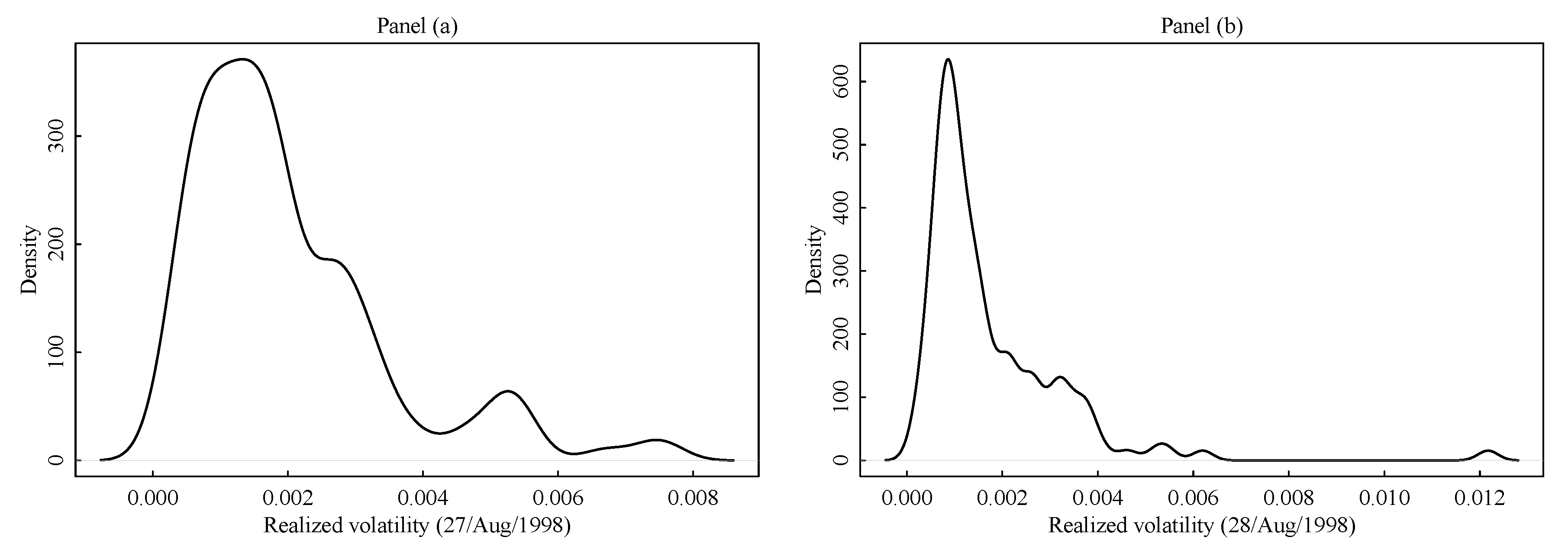
In this section, we introduce a model for the cross-sectional distribution of assets’ volatility. While considerable research has investigated the time-series structure of the volatility process and its relationships with market and the expected returns (see, among others, Campbell and Hentschel 1992; Glosten et al. 1993), the question of how the distribution of assets’ volatility looks like at a given time point has received less attention. The key assumption in this work is that, at a given time point, there are groups of assets whose volatility cluster together to form groups of homogeneous risk. This assumption has been already explored in Coretto et al. (2011). This is empirically motivated by analyzing cross-sectional realized volatility data. From the data set studied in Section 4 including 123 stocks traded on the New York Stock Exchange market (NYSE), in Figure 1 we show the kernel density estimate of the cross-sectional distribution of the realized volatility in two consecutive trading days.
Details on how the realized volatility is computed are postponed to Section 4. In both panels of Figure 1 there is evidence of multimodality, and this is consistent with the idea that there are groups of assets forming sub-populations with different average volatility levels. In panel (b) the kernel density estimate is corrupted by few assets exhibiting abnormal large realized volatility, this happens for a large number of trading days. In Figure 1b the two rightmost density peaks close to 0.006 and 0.012 each capture just few scattered points, although the plot seems to suggest the presence of two symmetric components. Not the kernel density estimator itself, but the estimate of the optimal bandwidth of Sheather and Jones (1991) used in this case is heavily affected by this typical right-tail behavior of the distribution. This sort of artifacts are common to other kernel density estimators. Unless a large smoothing is introduced, in the presence of scattered points in low density regions the kernel density estimate is mainly driven by the shape of the kernel function. On the other hand, increasing the smoothing would tarnish the underlying multimodality structure.
The cross-sectional structure discussed above is consistent with mixture models. The idea is that each mixture component represents a group of assets that share similar risk behaviour. Let h t , s be the realized volatility of the asset s at time t. We assume that at each t there are G groups of assets. Furthermore, conditional on D t , s , j = 1 , the jth group has a distribution f j ( · ) that is symmetric about the center m t , j , has a variance v t , j , and its expected size (proportion) is π t , j = E [ · | I t 1 ] . This implies that the the cross-sectional distribution of the realized volatility (unconditional on { D t , s , j } ) is represented by the finite location-scale mixture model
j = 1 G π t , j f j ( h t , s ; m t , j , v t , j ) .
The idea is that each mixture component represents a group of assets that share similar risk behaviour. The parameter m t , j represents the average within group realized volatility, while v t , j represents its dispersion. Mixture models can reproduce clustered population, and it is a popular tool in model-based cluster analysis (see Banfield and Raftery 1993; McLachlan and Peel 2000, among others). Coretto et al. (2011) exploited the assumed mixture structure for using robust model-based cluster analysis to group asset with similar risk, and they proposed a parsimonious multivariate dynamic model where aggregate clusters’ volatility is modeled instead of individual assets’ volatility. The main goal of their work was to reduce the unfeasible large dimensionality of multivariate volatility models for large portfolios. Clustering methods applied to financial time series were also used in Otranto (2008), where the autoregressive metric (see Corduas and Piccolo 2008) is applied to measure the distance between GARCH processes.
Finite mixtures of Gaussians, that is when f j ( · ) is the Gaussian density, are effective to model symmetrically shaped clusters also when clusters are not exactly normal. But in this case some more structure is needed to capture the effects of large variations in assets volatility that often show up for many trading days, e.g., the example shown in panel (b) of Figure 1. In Coretto et al. (2011) it was proposed to adopt the approach of Coretto and Hennig (2016, 2017) where an improper constant density mixture component is introduced to catch points (interpreted as noise or contamination) in low density regions. This makes sense in all those situations where there are points extraneous to each clusters that have an unstructured behavior, and that can potentially appear everywhere in the data space. This is not exactly the cases studied in this paper. In fact, realized volatility is a positive quantity, and this heterogeneous component can only affect the right tail of the distribution. Here we assume that the group of few assets inflating the right tail of the distribution have a proper uniform distribution whose support is not overlapping with the other regular volatility clusters. Let j = 0 denote this group of asset exhibiting “abnormal” large volatility, we call this group of points “noise”. The term noise here is inherited from the robust clustering and classification literature (see Ritter 2014), where it is understood as a “noisy cluster”, that is, a cluster of points with an unstructured shape compared with the main groups in the population. The uniform distribution is a convenient choice to capture atypical group of points not having a central location, and that are scattered in density regions somewhat separated from the main bulk of the data (Banfield and Raftery 1993; Coretto and Hennig 2016; Hennig 2004).
We assume that
h t , s | D t , s , 0 = 1 Uniform ( l t , u t ) h t , s | D t , s , j = 1 Normal ( m t , j , v t , j ) for j = 1 , G
where l t < u t are respectively the lower and upper limit of the support of the uniform distribution. The previous implies that, without conditioning on the class labels { D t , s , j } , the cross-sectional distribution of the assets’ volatility is represented by the following finite mixture model
f ( h t , s ; θ t ) = π t , 0 I { l t h t , s u t } u t l t + j = 1 G π t , j ϕ ( h t , s ; m t , j , v t , j ) ,
where ϕ ( · ) is Gaussian density function. The unknown mixture parameter vector is θ t = ( π t , 0 , l t , u t , π t , 1 , m t 1 , v t , 1 , , π t , G , m t G , v t , G ) . This class of models where introduced in Banfield and Raftery (1993), and studied in Coretto and Hennig (2010, 2011) to perform robust clustering. The additional problem here is that if θ t is unrestricted one may have situations where the support of the noise group overlaps with one or more regular clusters if l t is small enough. The latter would be inconsistent with the empirical evidence. To overcome this, we propose the following restriction, that is we assume that θ t is such that
m j , t + λ v j , t l t for all j = 1 , 2 , , G .
The constant λ > 0 controls the maximum degree of overlap between the support of the uniform distribution representing atypical observations and the closest regular Gaussian component. To see this, let z 0 . 99 be the 99% quantile of the standard normal distribution, and take λ = z 0 . 99 . The restriction (8) means that the uniform component can only overlap with the closest Gaussian component in its 1% tail probability. Restriction (8) now ensures a well separation between regular and non-regular assets.
Although the mixture model introduced in this section is interesting for how it is able to fit the cross-sectional distribution of realized volatility at each time period, the main issue here is to obtain the hard class memberships variables { D t , s , j } , and the smooth version { τ t , s , j } . Since τ t , s , j = Pr { D t , s , j = 1 | I t } , here we have that
τ t , s , j = π t , 0 I { l t h t , s u t } u t l t 1 f ( h t , s ; θ t ) if j = 0 , π t , j ϕ ( h t , s ; m t , j , v t , j ) f ( h t , s ; θ t ) if j = 1 , 2 , , G .
Quantities in (8) are obtained simply applying the Bayes rule, this the reason why these are also called “posterior weights” for class memberships. It can be easily shown (see Velilla and Hernández 2005, and references therein) that the optimal partition of the points can be obtained by applying the following assignment rule also called “Bayes classifier
D t , s , j * = I j = arg max j = 0 , 1 , , G { τ t , s , j } .
Basically the Bayes classifier assigns a point h t , s to the group with largest posterior probability of membership. The assignment rule in (10) is optimal in the sense that it achieves the lowest misclassification rate. Therefore, in order to obtain (10) and (9) from the data one needs to estimate θ t at each cross-section. Although we use the subscript t to distinguish the θ parameter in each cross-section, we do not assume any dependence in it. Here we treat the number of groups G as fixed an known. While in some situation, including the one studied in this paper, a reasonable value of G can be determined based on subject matter considerations, this is not always the case. In Section 4 we will motivate our choice of G = 3 for this study and we will give some insights on how to fix in it in general.
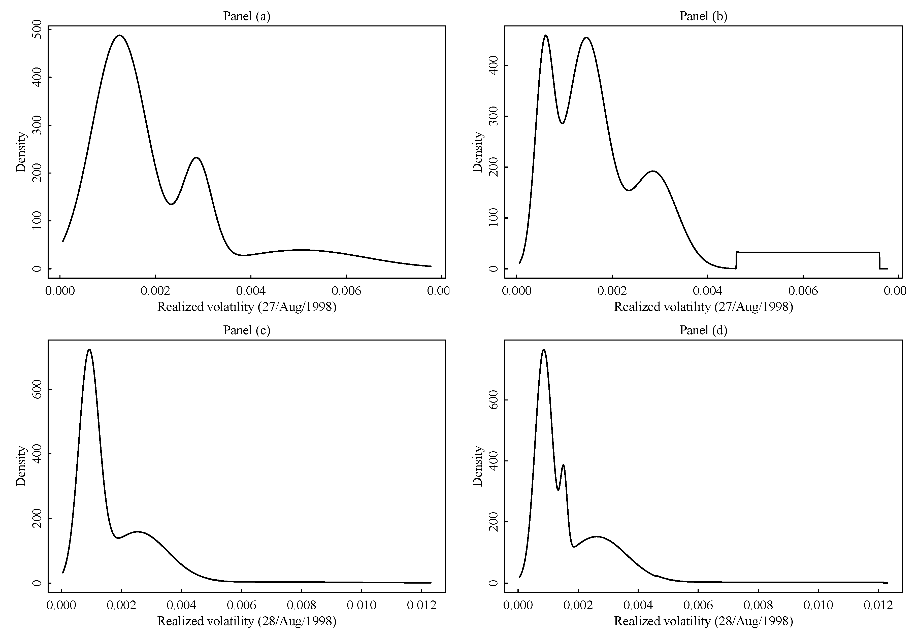
In the next Section 3 we introduce estimation methods for the quantities of interest, that are class memberships { D t , s , j } and smooth weights { τ t , s , j } . But before to conclude this session we show how model (7) under (8) fits the data sets of the example of Figure 1. In this paper we are mainly interested in the cluster structure of the cross-sectional data, however, it is also of interest to investigate the fitting capability of the cross-sectional model. Estimated density of the two data sets of example in Figure 1 are shown in Figure 2. Panel (a) and (b) of Figure 2 refers to the cross-section distribution of realized volatility on 27/Aug/1998 (compare with panel (a) in Figure 1). Panel (c) and (d) of Figure 2 refers to the cross-section distribution of realized volatility on 28/Aug/1998 (compare with panel (b) in Figure 1). In panel (a) and (c) of Figure 2 we show the fitted density based on model (7) with G = 3 under (8), and the additional restriction that π t , 0 = 0 , i.e., there is no uniform noise. In panels (b) and (d) the same model is fitted with the uniform component active. Comparing panels (a) and (b) of Figure 2 with panel (a) in Figure 1 one can see how the proposed model can lead to well separated components. The comparison of panels (a) and (b) in Figure 2 shows how the introduction of the uniform component completely modify the fitted regular components. In fact, in the case of panel (a) the absence of the uniform component causes a strong inflation of the variance of the rightmost Gaussian component so that the second component seen in panel (b) is completely eaten. A similar situation happen in panel (c) and (d) of Figure 2. Because of the uniform density in model (7) possible discontinuities at the boundaries of uniform support may arise in the final estimate. Compare Panel (d) vs. panel (b) in Figure 2. When the group of noisy assets is reasonably concentrated, the corresponding support of the fitted uniform distribution becomes smaller, and the uniform density easily dominates the tail of the closest regular distribution (e.g., this happens in panel (b)). The discontinuity of the model density is less noticeable in cases like the one in panel (d) where the support of the uniform is rather large because of extremely scattered abnormal realized volatility. Although the discontinuity introduced by the uniform distribution adds some technical issues for the estimation theory (see Coretto and Hennig 2011), it has two main advantages: (i) it allows to represent unstructured groups of points with a well defined, simple and proper probability model; (ii) the noisy cluster is understood as a group of points not having any particular shape, and that is different and distinguished from the regular clusters’ prototype model (the Gaussian density here). Therefore, a discontinuous transition between regular and non-regular density region obeys to the philosophy in robust statistic that in order to identify outliers/noise they need to arise in low density regions under the model for the regular points. Further discussions about the model-based treatment of noise/outliers in clustering can be found in Hennig (2004) and Coretto and Hennig (2016).

3. Estimation

The main goal of this paper is to estimate models (1) and (4). If the class membership variables { D t , s , j } or the posterior weights { τ t , s , j } were known, one could have estimated the unknown parameter by optimizing the sample log-likelihood function of (1) or (4). However, both { D t , s , j } and { τ t , s , j } are not known. In Section 2.2 we developed a model for the cross-sectional distribution of the realized volatility, and an unknown parameter vector θ t controls this distribution at each time point. It may be possible to embed both the time series model, and the cross-sectional model in a single likelihood function and proceed with a single Maximum Likelihood (ML) estimation. Although this is in principle possible, it would lead to an unfeasible optimization problem. Since we assume that at each time point the time series model (1) (or (4)) does interact with the current values of { D t , s , j } (or { τ t , s , j } ), we propose to simplify the estimation in two separate steps:
Step 1:
using cross-sectional data on realized volatility, at each time period the parameter θ t is estimated based on ML. The fitted θ t is used to obtain an estimates of { D t , s , j * } and { τ t , s , j } based on (9) and (10).
Step 2:
the ML (or quasi-ML) method applied to estimate the unknown parameters of (1) or (4).
Step 1 is performed by solving the following constrained ML program
maximize θ t s = 1 S log f ( h s , t ; θ t ) , subject to 0 < v min v j , t , for j = 1 , 2 , , G , 0 < v min ( u t l t ) 2 / 12 , m j , t + λ v j , t l t , for j = 1 , 2 , , G .
Let θ ^ t the solution of the previous ML program. Additionally to the model constraint introduced in (8), the proposed ML optimization has two further constraints that require the specification of positive constant v min . This is a lower bound for the variance of both types of mixture components (e.g., the Gaussian and the uniform). It is well known that the unconstrained ML for mixture of location-scales distribution does not exist, and in practice it can easily leads to spurious solutions (see McLachlan and Peel 2000; Redner and Walker 1984, among the others). In our study we set v min = 10 5 , while we take λ = z 0 . 99 as explained in Section 2.2. The numerical solution of (11) is complicated by the discontinuities introduced by the uniform component, and the additional constraint implementing (8). The Expectation-Maximization (EM) algorithm proposed in Coretto and Hennig (2011) can be easily adapted to obtain θ ^ t . Based on θ ^ t the corresponding { D ^ t , s j } and { τ ^ t , s , j } are computed by plugging in θ ^ t into (9) and (10).
In Step 2, conditional on the estimated memberships, { D ^ t , s j } and { τ ^ t , s , j } , for any asset s, the parameters of the model for returns, ψ s = ( μ s , ω s , α s , β s ) , are estimated maximizing the conditional likelihood function
maximize ψ s t = 1 T log ϕ ( r t , s | I t 1 , L s , t 1 ; ψ s ) , subject to ω j > 0 , for j = 1 , 2 , , G , α j 0 , for j = 1 , 2 , , G , β j 0 , for j = 1 , 2 , , G .
where ϕ ( x | . ) denotes the conditional density of X, L s , t 1 = g t , s , for the CW-GARCH model, and L s , t 1 = τ t , s , for the sCW-GARCH model. In order to gain some insight on the statistical properties of the estimation procedure for the dynamic volatility coefficients, we have performed a Monte Carlo simulation study. Namely, first, conditional on appropriately selected state variables g t , s (see below), we have generated n s i m = 500 time series of length T = 2500 , taking the CW-GARCH as Data Generating Process (DGP). The same model has then been fitted to each of these series maximizing the conditional likelihood function in (12). Further, the described simulation procedure has been implemented taking the sCW-GARCH model as DGP, again conditioning on appropriately selected state variables τ t , s . In order to facilitate the comparison of results across different DGPSs, the same vector of volatility coefficients ψ has been used for simulating from both CW-GARCH and sCW-GARCH.
The length of the simulated series has been selected to match the time series dimension of the panel analyzed in Section 4. We note that the models proposed in this paper are conditional to the state variables g t , s and τ t , s . In practical applications, these are not observed and, in fact, the cross-sectional clustering algorithm is introduced in order to recover them. In order to a have a sampling design that is consistent with the empirical evidence, the simulation uses input state variables the g t , s and τ t , s obtained from applying the clustering algorithm (11) on carefully selected stocks in the panel studied in Section 4. We recall that models (2) and (4) contain the GARCH(1,1) model as a nested case if an asset does not migrate across states, but stays stably in one of the volatility clusters. In order to have a sampling representing maximum heterogeneity, we looked for the g t , s and τ t , s of an asset with the distribution over the states {low, medium, high, noise} having maximal entropy. This particular selection guarantees that the state variables g t , s and τ t , s used as input for the simulation, represent the dynamics of an asset that travels uniformly across the states. The same GARCH-type parameter vector, corresponding to the the ψ –row in Table 1, have been fixed to simulate both (2) and (4). While there exists an extensive empirical literature about the classical GARCH(1,1) model, so that it is known what a realistic parameter should be picked for a numerical experiment, this obviously does not apply to models (2) and (4) proposed in this paper. Therefore we decided to fix ψ as a perturbation of the median behavior (across the market) obtained from the in-sample results in Section 4.1.
The simulation results, summarized in Table 1, support the following facts. First, for both DGPs, the estimates are on average close to the DGP coefficients. Second, in general, the simulated Root Mean Squared Errors (RMSE) are, in relative terms, small, compared to the level of the underlying coefficient. Finally, no clear ordering of the two models arises in terms of efficiency in the estimation of model parameters.
2pt

4. Empirical Study

Our data set is composed of 5-min log-returns for 123 assets traded on the NYSE from 11/Aug/1998 to 18/Jul/2008 for a total of 2500 trading days. The assets have been selected in order to guarantee the (i) availability of a sufficiently long time-span; (ii) maximize liquidity over the time period of interest. 5-min returns have then been aggregated on a daily scale to compute daily Realized Variances on open-to-close log-returns.
For the step 1 of the estimation we fix G = 3 . G is an important decision, and rarely is determined from the data alone. Although there is large collection of methods to select an appropriate number of clusters, a consensus in the literature has not been reached. In the model-based clustering context a popular choice is to select G based on the BIC, or alternative information criteria (for a comprehensive review see McLachlan and Peel 2000). However, none of the existing methods have strong theoretical guarantees, and often, it makes more sense to supervise the choice of G based on subject-matter considerations additional to data-driven methods (Hennig and Liao 2013; Hennig et al. 2016). The choice of G = 3 is motivated based on various arguments. First of all we considered G ranging from 2 to 6 and we looked at many cross-sectional fit at random (as in Figure 2). The BIC criterion always suggested G = { 3 , 4 } , a supervised analysis of the results confirmed that meaningful cross-sectional fits were always obtained with G = 3 or G = 4
. We also explored the opinion of several professional financial analysts, and the general conclusion is that a classification into low-medium-high risk is the conventional operational way to categorize risk. Our cross-sectional model (7) also includes an atypical component for catching extremely large risk levels. Therefore we finally considered G = 3 and G = 4 , and based on the performance of the forecasting experiment described in Section 4.2, we finally decided that G = 3 is the appropriate number of regular groups to consider because G = 3 produced the overall lowest average (across assets) Root Mean Square Prediction Error (RMSPE). Details about forecasting performance are treated in Section 4.2. Selection of a G value that optimizes the predictive performance is an appropriate way to approach the selection of G when the main goal is to predict future volatility. For each cross-sectional fit of θ t the mixture component are always ordered in terms of increasing risk. Therefore the groups j = 1 , 2 , 3 always correspond to groups of increasing average realized volatility. In other words, the cluster indexes js are rearranged so that m t , 1 m t , 2 m t , 3 , and in case of equal means the order is based on variances v t , j , and for equal variances the order based on the expected size π t , j . We refer to the groups corresponding to j = 1 , 2 , 3 as group = low, medium, high. The group identified with j = 0 is called noise, and in the ordering scheme is placed after the high group because in this empirical application it always captures overall highest volatility assets. For the noise component, an indexing alternative to j = 0 may be decided, although in principle outlying points can be everywhere in the data range, and the uniform component may well catch small outliers or inliers (see Coretto and Hennig 2010). In the robust clustering literature it is common to denote the noise component with j = 0 so that G still defines the number of regular clusters.
Step 2 of the estimation procedure is performed considering a Gaussian Quasi-Likelihood function, that is we set
log ϕ ( r t , s | I t 1 , L s , t 1 ; ψ s ) = 1 2 log ( σ t , s 2 ) 1 2 log ( 2 π ) ( r t , s μ s ) 2 σ t , s 2 ,
leading to the following expression for the overall Quasi-Likelihood
log ( r s | ψ s ) = t = 1 T log ϕ ( r t , s | I t 1 , L s , t 1 ; ψ s ) = 1 2 t = 1 T log ( σ t , s 2 ) T 2 log ( 2 π ) 1 2 t = 1 T ( r t , s μ s ) 2 σ t , s 2 .
Maximizing (14) with respect to ψ s , for any asset s, leads to consistent and asymptotically Normal estimates of ( μ s , ω s , α s , β s ) even when the conditional returns distribution in (13) is not correctly specified (Bollerslev and Wooldridge 1992).

4.1. In-Sample Results

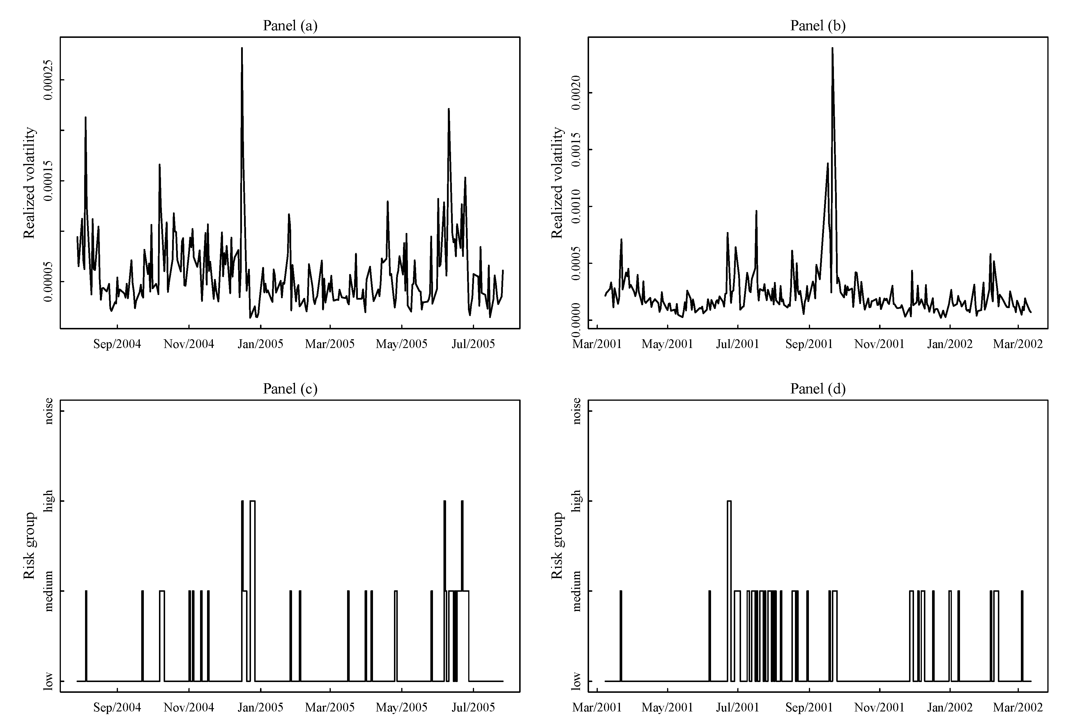
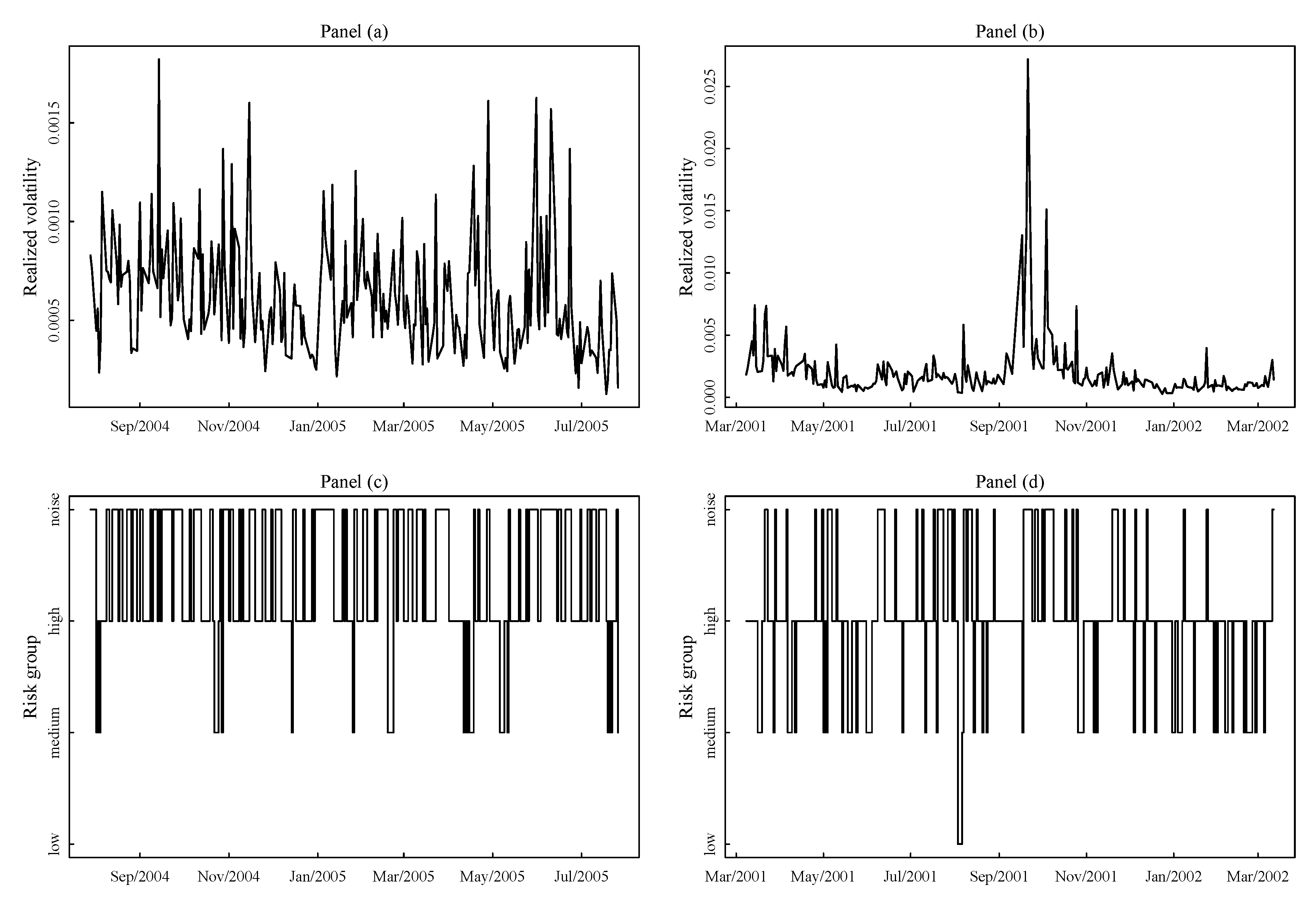
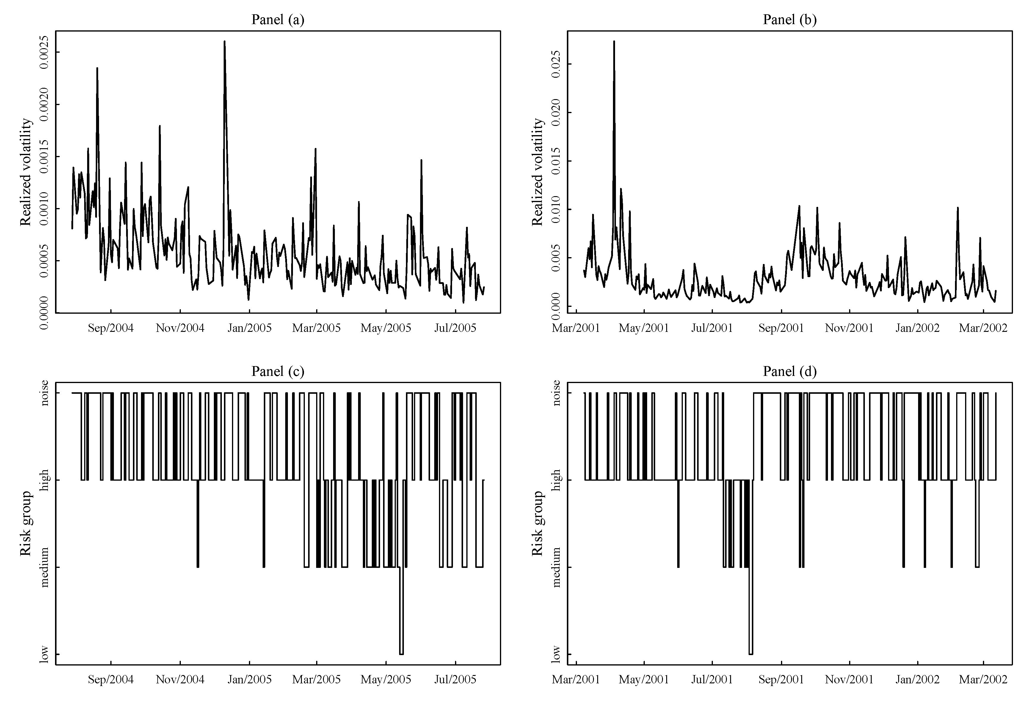
The cross-sectional estimation showed that there are various interesting patterns in the data. Assets migrate from one risk group to another over time, but these class switch dynamics show a strong dose of persistence In Figure 3, Figure 4 and Figure 5 we show time series of the realized volatility and class switches for three assets, e.g., asset JNJ, asset LSI, and asset NOVL. For each asset we consider two period of 365 days: the period August 2004–August 2005 for the lowest overall market volatility in our sample, and the period March 2001–March 2002 for the largest overall market volatility. Each of the Figure 3, Figure 4 and Figure 5 corresponds to an asset, panels (a) and (b) refers to the low volatility period, panels (b) and (d) show the large volatility period. In Figure 3 we note that asset JNJ persistently stays in the low class of risk, and eventually it switches to the next medium group for short time intervals when the market volatility bumps up. The interesting thing to observe is that this behavior is almost the same in the two periods, e.g., the dynamic of these switches does not depend from the level of the market volatility. As expected in the high volatility period the persistence in the low group decreases, but overall the pattern is rather stable. If we count the number of changes from one class to another, asset JNJ is the most stable asset overall with the longest permanence in the low risk group. On the other hand asset LSI in Figure 4 was chosen because it is the most unstable, i.e., it is the asset with the largest number of jumps from one class to another. This asset has a less persistent dynamic in terms of class switches. The interesting thing is that this asset stay more in the lower risk group when the market volatility increases. A different pattern is observed for asset NOVL in Figure 5. asset NOVL, as asset LSI, has a strong tendency to stay in high risk group with a preference for the noise group. However, contrary to asset LSI, asset NOVL increases its stay in the noise group as the market volatility increases. The cross-sectional clustering step also transform a cardinal quantity like volatility into an ordinal variable much easier to interpret. One of the advantage of such a categorization of the volatility is that it is market contingent. These graphical plots of the class switches may be of practical interests for financial analyst. This is an interesting application itself maybe worth to be explored in more details in further research.
Moving our attention to the results of Step 2 of the estimation procedure, Table 2 reports the average and median values of the second stage conditional log-likelihood and of the Bayesian Information Criterion (BIC) for CW-GARCH, sCW-GARCH and two benchmarks given by the GARCH and GJR models of order (1,1), respectively. We remind that the volatility equation of a GJR(1,1) model (Glosten et al. 1993) is given by
σ t , s 2 = ω s + α s ( r t 1 , s μ s ) 2 + β s σ t 1 , s 2 + γ s ( r t 1 , s μ s ) 2 I ( ( r t 1 , s μ s ) < 0 ) ,
where the additional γ coefficients controls for leverage effects. In particular, the occurrence of leverage effects is associated to positive values of the coefficient. The GARCH(1,1) model is nested within the GJR specification for γ = 0 .
The CW-GARCH and sCW-GARCH models are clearly outperforming the benchmarks in terms of both average and median BIC, with the sCW-GARCH being the best performer. As expected, the GJR-GARCH outperforms the simpler GARCH model.
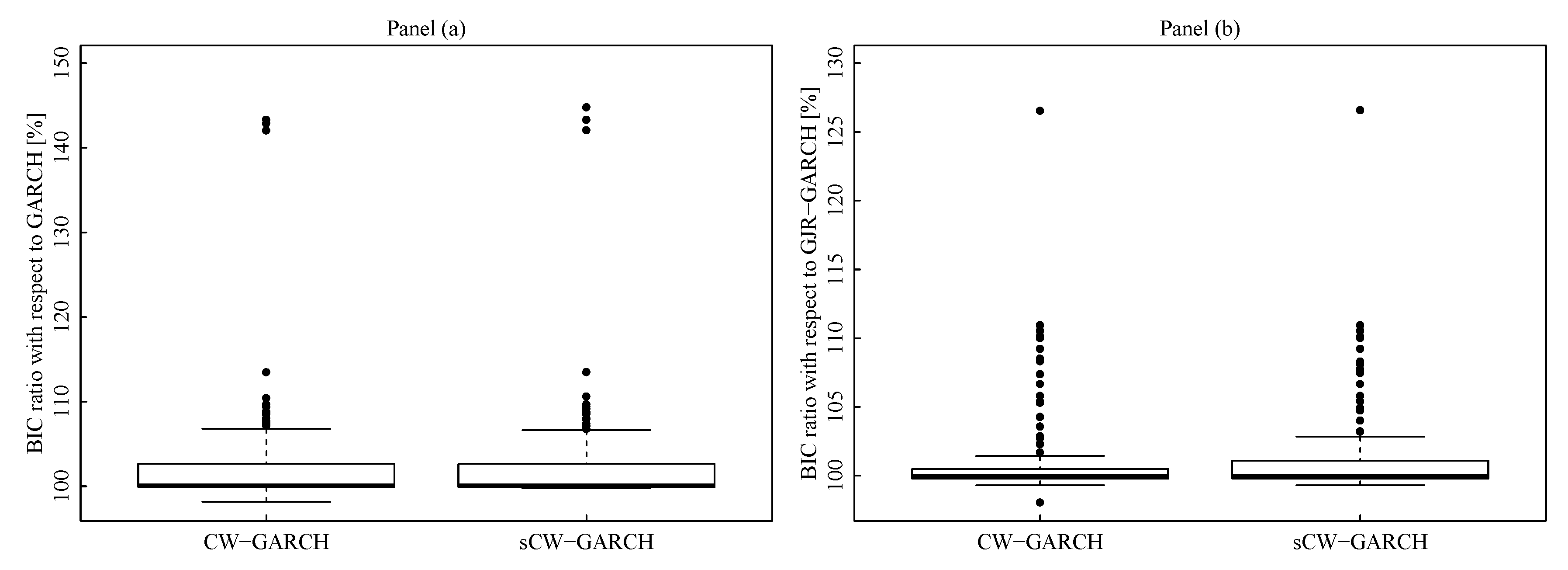
The picture is completed by the analysis of Figure 6 that the reports the box-plots of the ratios between the BIC values of CW-GARCH and sCW-GARCH, in the numerator, and those of the benchmarks, in the denominator. For ease of presentation, the ratios have been multiplied by 100 so that, in the plot, values above 100 indicate that the benchmark is outperformed by the model in the numerator. The plot makes evident that, in the vast majority of cases, CW-GARCH and sCW-GARCH perform better than GARCH and GJR models. Also, while there are several assets for which the CW-GARCH and sCW-GARCH are doing remarkably better than the benchmarks (in some cases the gain in BIC is above 40%, for the GARCH, and above 25%, for the GJR), the reverse does not hold.
Finally, it is interesting to look at the average (Table 3) and median (Table 4) estimated coefficients across the whole set of 123 assets. For both CW-GARCH and sCW-GARCH, some regularitites arise. First and most importantly, the α coefficient tends to decrease as we move from low to high volatility components, taking its minimum value for the noise component. This implies that the impact of past squared returns tends to be down-weighted as the relative volatility level increases. Intuitively, this effect reaches its extreme level in the case of the noise component when it is reasonable to expect that the current returns do not offer a strong signal for the prediction of future conditional variance. Accordingly, the volatility persistence ( α + β ) also takes its minimum value for the noise component.
In addition, since the GARCH model can be obtained as a special case of the CW-GARCH model, we test the signficance of the likelihood gains yielded by the latter model via a Likelihood Ratio Test (LRT). The p-values of the LRT test, for all the 123 assets included in our panel, have been graphically represented in Figure 7. In order to improve the readability of the plot, we have transformed the p-values on a logit scale. The null hypothesis is rejected at any reasonable significance level for 122 assets out of 123.

4.2. Forecasting Experiments

In order to assess the ability of the proposed models to generate accurate one-step-ahead volatility forecasts, we have performed an out-of-sample forecasting exercise based on a mixed-rolling window design with re-estimation every 50 observations over a moving window of 1500 days, implying 20 re-estimation for each asset. So, the first 1500 observations have been taken as initial sample period while the last 1000 have been kept for out-of-sample forecast evaluation. As for the in-sample analysis, the GARCH(1,1) and GJR(1,1) models are considered as benchmarks.
For clarity, for a generic asset s, the structure of the forecasting design can be summarized in the following steps
  • Using observation from 1 to 1500, fit a CW-GARCH, sCW-GARCH, GARCH and GJR-GARCH model to the time series of returns on asset s
  • Generate one-step-ahead forecasts of conditional variance for the subsequent 50 days, that is for times 1501 to 1550
  • Re-estimate the models using an updated estimation window from 51 to 1550
  • Iterate steps 2-3 until the end of the series.
The series of forecasts obtained by the three models considered are then scored using two different performance measures: the Root Mean Squared Prediction Error (RMSPE) and the QLIKE loss (Patton 2011). Letting, h t be the realized volatility at time t and σ ^ t , k 2 the conditional variance predicted by model k where k { GARCH , GJR GARCH , CW GARCH , sCW GARCH } , the RMSPE and QLIKE for model k are given by
RMSPE k : = avg j σ ^ T + j , k 2 h T + j , k 2 ,
QLIKE k : = avg j log ( σ ^ T + j , k 2 ) + h T + j 2 σ ^ T + j , k 2 ,
for T = 1500 and j = 1 , , 1000 . In both cases, lower average values of the loss will be associated to better performers. Both the RMSPE and QLIKE are strictly consistent for the conditional variance of returns and can be shown to be robust to the quality of the volatility proxy used for forecast evaluation. The results of the forecasting comparison for all the 123 assets included in our data set have been summarized in Table 5 that, for both RMSPE and QLIKE, reports the percentage of times that each of the models considered has been found to be the best performer. Here, slightly different pictures are obtained under the RMSPE and QLIKE losses, respectively. Under the RMSPE loss, the CW-GARCH model is resulting the best performer for approximately 1/3 of the assets while the remaining models are characterized by very close performances, with the GJR-GARCH slightly outperforming the GARCH and sCW-GARCH models. Overall, a state dependent models, either the CW-GARCH or sCW-GARCH model, results to be the best performer for approximately 55% of the assets. Under the QLIKE loss, no clear winner arises. The GJR-GARCH and CW-GARCH give very close “winning” frequencies, with the first slightly outperforming the latter. Overall, one of the state-dependent models results to be the best performer for approximately 50% of the assets.
Although looking the “winning” frequencies offers a simple and tempting way of summarizing the forecasting performance of different models across a large number of assets, it should be remarked that this approach does not allow to consistently rank models according to their overall “aggregate” forecasting performance since “winning” frequencies do not incorporate any information on a cardinal measure of the model’s predictive ability.
To overcome this limit, Table 6 provides a summary of the RMSPE and QLIKE distributions across the 123 assets included in our panel. Namely, the table shows that the median loss is substantially lower for CW-GARCH and sCW-GARCH models than for the benchmarks. The performance gap appears more evident for the RMSPE than for the QLIKE. Furthermore, compared to the GARCH and GJR-GARCH models, the CW-GARCH and sCW-GARCH models are characterized by more stable forecasting performances, as documented by the value of the InterQuartile Range (IQR) for both RMSPE and QLIKE.
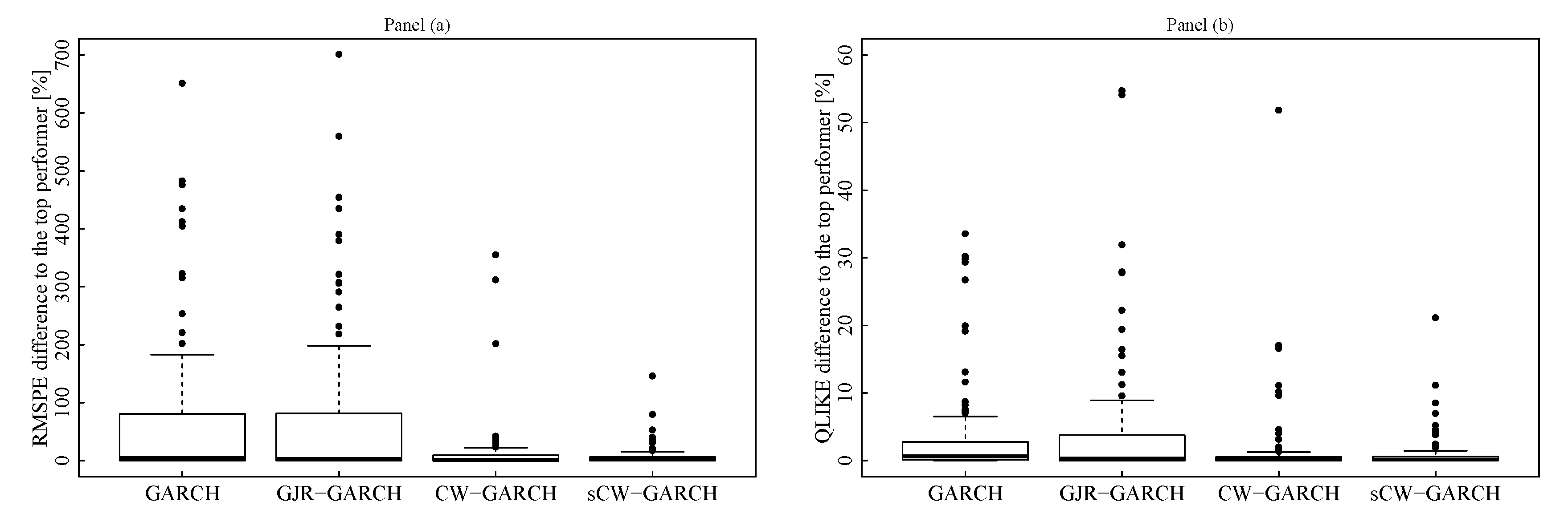
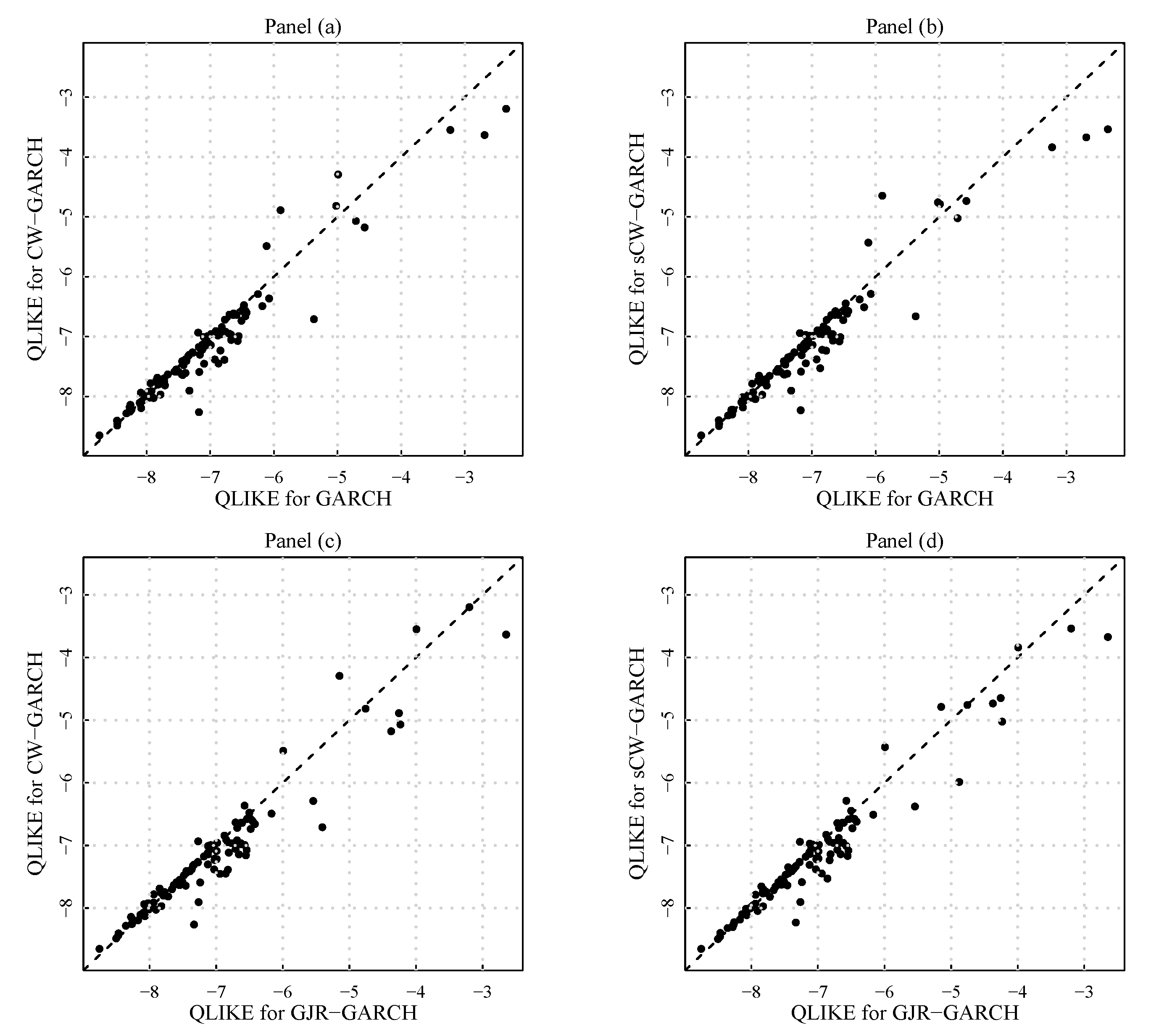
Figure 8 reports, for each model, the boxplot of the percentage differences between the loss value yielded by the model and that registered for the top performer for a given asset. The plots clearly show that these gaps tend to be smaller for CW-GARCH and sCW-GARCH models rather than for the benchmarks. Our findings on the distribution of performance gaps among the four models considered are further investigated and confirmed by Figure 9, for the RMSPE, and Figure 10, for the QLIKE. In each figure the first two plots compare, the average loss yielded by the CW-GARCH and sCW-GARCH, respectively, on the y-axis, with the average obtained for the GARCH models. The two scatter-plots in the second row repeat the comparison replacing the GARCH with the GJR model on the x-axis.
Finally, as a further robustness check we have computed the Diebold-Mariano statistic (Diebold and Mariano 1995) in order to test the null hypothesis of Equal Predictive Ability (EPA) of CW-GARCH and sCW-GARCH against the two benchmarks given by GARCH and GJR-GARCH, respectively. The results of our testing exercise have been summarized in Table 7. Here, by % L we denote the percentage of assets for which the average MSPE of the benchmark (GARCH or GJR-GARCH) is lower than that of CW-GARCH or sCW-GARCH model, respectively. In parentheses, below the above value, we report the percentage of times in which this corresponded to a significant Diebold-Mariano test statistic the usual 5% level. Similarly, % W indicates the percentage of assets for which the average MSPE of the CW-GARCH or sCW-GARCH is lower than that of the benchmark. For example, when the GARCH is taken as a benchmark, the average MSPE of GARCH is lower than that yielded by CW-GARCH in approx. 28.5% of cases, corresponding to 35 assets. In addition, for 80% of these assets, corresponding to 28 stocks, the Diebold-Mariano test rejects the null of EPA at the 5% level.
The results of our analysis reveal that, in the vast majority of cases ( 70 % ), both CW-GARCH and sCW-GARCH yield an average MSPE that is lower than that of the benchmarks. Furthermore, in over 80% of cases, this leads to a rejection of the EPA hypothesis at the 5% significance level.

5. Conclusions and Final Remarks

We have presented a novel approach to forecasting volatility for large panels of assets. Compared to existing approaches, our modelling strategy has some important advantages. First, conditional on the information on the group structure, inference is based on a computationally feasible two-stage procedure. This implies that the investigation of the multivariate group structure of the panel, performed in Stage 1, is separated from the fitting of the dynamic volatility forecasting models, that is performed in Stage 2. The desirable consequence of this architecture is that, at Stage 2, it is possible to incorporate multivariate information on the cross-sectional volatility distribution, without having to face the computational complexity of multivariate time series modelling.
Second, for a given stock, the fitted volatility forecasting model has coefficients that are asset specific and time-varying. Last but not least, the structure of our modelling approach is inherently flexible and can be easily adapted to consider alternative choices of the clustering variables as well as of the second-stage parametric specifications used for volatility forecasting. For example, the GARCH specification of the latent components of the CW-GARCH and sCW-GARCH could be easily replaced by other conditional heteroskedastic models such as, for example, GJR (Glosten et al. 1993) or even more sophisticated Realized GARCH models (Hansen et al. 2012), directly using information on realized volatility measures for conditional variance forecasting. On an empirical ground, both in-sample and out-of-sample results, provide strong evidence that the proposed approach is able to improve over simple univariate GARCH-type models, thus confirming the intuition that taking into account the information on the group structure of volatility can be profitable in terms of predictive accuracy in volatility forecasting.

Author Contributions

All authors contributed equally to this manuscript. All authors have read and agreed to the published version of the manuscript.

Funding

This research received no external funding.

Acknowledgments

The authors would like to thank two anonymous Referees for their stimulating comments and suggestions that helped us to enhance the quality of our paper.

Conflicts of Interest

The authors declare no conflict of interest.

Abbreviations

the following abbreviations are used in this manuscript:
GARCHGeneralized autoregressive conditional heteroskedasticity
GJR-GARCHGJR model proposed by Glosten et al. (1993)
CW-GARCHClusterwise generalized autoregressive conditional heteroskedasticity
sCW-GARCHSmooth CW-GARCH
NYSENew York Stock Exchange
MLMaximum Likelihood
RMSPERoot mean square prediction error
QLIKELoss function proposed by Patton (2011)

References

  1. Banfield, Jeffrey D., and Adrian E. Raftery. 1993. Model-based gaussian and non-gaussian clustering. Biometrics 49: 803–21. [Google Scholar] [CrossRef]
  2. Barigozzi, Matteo, Christian Brownlees, Giampiero M. Gallo, and David Veredas. 2014. Disentangling systematic and idiosyncratic dynamics in panels of volatility measures. Journal of Econometrics 182: 364–84. [Google Scholar] [CrossRef] [Green Version]
  3. Bauwens, Luc, and Jeroen Rombouts. 2007. Bayesian clustering of many GARCH models. Econometric Reviews 26: 365–86. [Google Scholar] [CrossRef]
  4. Bauwens, Luc, and Giuseppe Storti. 2009. A Component GARCH Model with Time Varying Weights. Studies in Nonlinear Dynamics & Econometrics 13: 1–33. [Google Scholar]
  5. Bollerslev, Tim. 1986. Generalized autoregressive conditional heteroskedasticity. Journal of Econometrics 31: 307–27. [Google Scholar] [CrossRef] [Green Version]
  6. Bollerslev, Tim, and Jeffrey M. Wooldridge. 1992. Quasi-maximum likelihood estimation and inference in dynamic models with time-varying covariances. Econometric Reviews 11: 143–72. [Google Scholar] [CrossRef]
  7. Campbell, John Y., and Ludger Hentschel. 1992. No news is good news. Journal of Financial Economics 31: 281–318. [Google Scholar] [CrossRef] [Green Version]
  8. Corduas, Marcella, and Domenico Piccolo. 2008. Time series clustering and classification by the autoregressive metric. Computational Statistics Data Analysis 52: 1860–72. [Google Scholar] [CrossRef]
  9. Coretto, Pietro, and Christian Hennig. 2010. A simulation study to compare robust clustering methods based on mixtures. Advances in Data Analysis and Classification 4: 111–35. [Google Scholar] [CrossRef]
  10. Coretto, Pietro, and Christian Hennig. 2011. Maximum likelihood estimation of heterogeneous mixtures of gaussian and uniform distributions. Journal of Statistical Planning and Inference 141: 462–73. [Google Scholar] [CrossRef]
  11. Coretto, Pietro, and Christian Hennig. 2016. Robust improper maximum likelihood: Tuning, computation, and a comparison with other methods for robust gaussian clustering. Journal of the American Statistical Association 111. [Google Scholar] [CrossRef]
  12. Coretto, Pietro, and Christian Hennig. 2017. Consistency, breakdown robustness, and algorithms for robust improper maximum likelihood clustering. Journal of Machine Learning Research 18: 1–39. [Google Scholar]
  13. Coretto, Pietro, Michele La Rocca, and Giuseppe Storti. 2011. Group structured volatility. In New Perspectives in Statistical Modeling and Data Analysis: Proceedings of the 7th Conference of the Classification and Data Analysis Group of the Italian Statistical Society, Catania, September 9–11, 2009. Edited by S. Ingrassia, R. Rocci and M. Vichi. Berlin/Heidelberg: Springer, pp. 329–35. [Google Scholar] [CrossRef]
  14. Creal, Drew, Siem Jan Koopman, and André Lucas. 2013. Generalized autoregressive score models with applications. Journal of Applied Econometrics 28: 777–95. [Google Scholar] [CrossRef] [Green Version]
  15. Diebold, Francis X., and Roberto S. Mariano. 1995. Comparing predictive accuracy. Journal of Business & Economic Statistics 13: 253–63. [Google Scholar] [CrossRef] [Green Version]
  16. Engle, Robert, Eric Ghysels, and Bumjean Sohn. 2013. Stock market volatility and macroeconomic fundamentals. The Review of Economics and Statistics 95: 776–97. [Google Scholar] [CrossRef]
  17. Engle, Robert, and Jose Rangel. 2008. The spline-garch model for low-frequency volatility and its global macroeconomic causes. Review of Financial Studies 21: 1187–222. [Google Scholar] [CrossRef]
  18. Engle, Robert F., Olivier Ledoit, and Michael Wolf. 2019. Large dynamic covariance matrices. Journal of Business & Economic Statistics 37: 363–75. [Google Scholar] [CrossRef] [Green Version]
  19. Gallo, Giampiero M., and Edoardo Otranto. 2018. Combining sharp and smooth transitions in volatility dynamics: A fuzzy regime approach. Journal of the Royal Statistical Society Series C 67: 549–73. [Google Scholar] [CrossRef] [Green Version]
  20. Glosten, Lawrence R., Ravi Jagannathan, and David E. Runkle. 1993. On the relation between the expected value and the volatility of the nominal excess return on stocks. Journal of Finance 48: 1779–801. [Google Scholar] [CrossRef]
  21. Hamilton, James, and Raul Susmel. 1994. Autoregressive conditional heteroskedasticity and changes in regime. Journal of Econometrics 64: 307–33. [Google Scholar] [CrossRef]
  22. Hansen, Peter Reinhard, Zhuo Huang, and Howard Howan Shek. 2012. Realized garch: A joint model for returns and realized measures of volatility. Journal of Applied Econometrics 27: 877–906. [Google Scholar] [CrossRef]
  23. Hennig, Christian. 2004. Breakdown points for maximum likelihood estimators of location–scale mixtures. The Annals of Statistics 32: 1313–40. [Google Scholar] [CrossRef] [Green Version]
  24. Hennig, Christian, and Tim F. Liao. 2013. How to find an appropriate clustering for mixed-type variables with application to socio-economic stratification. Journal of the Royal Statistical Society: Series C (Applied Statistics) 62: 309–69. [Google Scholar] [CrossRef] [Green Version]
  25. Hennig, Christian, Marina Meila, Fionn Murtagh, and Roberto Rocci. 2016. Handbook of Cluster Analysis. Boca Raton: CRC Press. [Google Scholar]
  26. Marcucci, Juri. 2005. Forecasting stock market volatility with regime-switching garch models. Studies in Nonlinear Dynamics & Econometrics 9: 1–55. [Google Scholar]
  27. McLachlan, Geoffrey J., and David Peel. 2000. Finite Mixture Models. New York: Wiley. [Google Scholar]
  28. Otranto, Edoardo. 2008. Clustering heteroskedastic time series by model-based procedures. Computational Statistics Data Analysis 52: 4685–98. [Google Scholar] [CrossRef] [Green Version]
  29. Pakel, Cavit, Neil Shephard, and Kevin Sheppard. 2011. Nuisance parameters, composite likelihoods and a panel of garch models. Statistica Sinica 21: 307–29. [Google Scholar]
  30. Patton, Andrew. 2011. Volatility forecast comparison using imperfect volatility proxies. Journal of Econometrics 160: 246–56. [Google Scholar] [CrossRef] [Green Version]
  31. Redner, Richard, and Homer F. Walker. 1984. Mixture densities, maximum likelihood and the EM algorithm. SIAM Review 26: 195–239. [Google Scholar] [CrossRef]
  32. Ritter, Gunter. 2014. Robust Cluster Analysis and Variable Selection. Monographs on Statistics and Applied Probability. New York: Chapman and Hall/CRC. [Google Scholar]
  33. Sheather, Simon J., and Michael C. Jones. 1991. A reliable data-based bandwidth selection method for kernel density estimation. Journal of the Royal Statistical Society. Series B. Methodological 53: 683–90. [Google Scholar] [CrossRef]
  34. Velilla, Santiago, and Adolfo Hernández. 2005. On the consistency properties of linear and quadratic discriminant analyses. Journal of Multivariate Analysis 96: 219–36. [Google Scholar] [CrossRef] [Green Version]
Figure 1. For the data set introduced in Section 4 it is shown the kernel density estimate of the cross-sectional distribution of realized volatility in two different time points: panel (a) refers to 27 August 1998; panel (b) refers to 28 August 1998.
Jrfm 13 00064 g001
Figure 2. Parametric density estimate of the cross-sectional distribution for that data sets of the example in Figure 1. (a) Realized volatility on 27/Aug/1998; fitted density based on model (7) with G = 3 , under the restriction (8) and that π 0 = 0 (that is the uniform component is inactive). (b) Realized volatility on 27/Aug/1998; fitted density based on model (7) with G = 3 , under the restriction (8). (c) Realized volatility on 28/Aug/1998; fitted density based on model (7) with G = 3 , under the restriction (8) and that π 0 = 0 (uniform component is inactive). (d) Realized volatility on 28/Aug/1998; fitted density based on model (7) with G = 3 , under the restriction (8).
Jrfm 13 00064 g002
Figure 3. (a) Time series of the realized variance of asset JNJ from August 2004 to August 2005. (b) Sequence of fitted class labels memberships for the asset JNJ from August 2004 to August 2005. (c) Time series of the realized variance of asset JNJ from March 2001 to March 2002. (d) Sequence of fitted class labels memberships for the asset JNJ from March 2001 to March 2002.
Jrfm 13 00064 g003
Figure 4. (a) Time series of the realized variance of asset LSI from August 2004 to August 2005. (b) Sequence of fitted class labels memberships for the asset LSI from August 2004 to August 2005. (c) Time series of the realized variance of asset LSI from March 2001 to March 2002. (d) Sequence of fitted class labels memberships for the asset LSI from March 2001 to March 2002.
Jrfm 13 00064 g004
Figure 5. (a) Time series of the realized variance of asset NOVL from August 2004 to August 2005. (b) Sequence of fitted class labels memberships for the asset NOVL from August 2004 to August 2005. (c) Time series of the realized variance of asset NOVL from March 2001 to March 2002. (d) Sequence of fitted class labels memberships for the asset NOVL from March 2001 to March 2002.
Jrfm 13 00064 g005
Figure 6. (a) Boxplots of the distribution (across the portfolio) of the ratio (BIC achieved by a given model)/(BIC achieved by the GARCH(1,1) model), where the ratio is scaled in percentage value. Each data point is a BIC-ratio for model (1) or (4) achieved by one of the S = 123 assets in the sample. (b) Boxplots of the distribution (across the portfolio) of the ratio (BIC achieved by a given model)/(BIC achieved by the GJR-GARCH(1,1) model), where the ratio is scaled in percentage value. Each data point is a BIC-ratio for model (1) or (4) achieved by one of the S = 123 assets in the sample.
Jrfm 13 00064 g006
Figure 7. p-values of the Likelihood Ratio Test (LRT) test of CW-GARCH vs. GARCH for all the 123 assets included in our panel. The y-axis of the plot is scaled in terms of logit(p-value), y-axis labels are shown as percentage p-values.
Jrfm 13 00064 g007
Figure 8. For each loss and each method, it is shown the distribution (across the S = 123 assets) of the percentage difference between the loss of the method and the loss of the top performer, relative to the size of the loss of the top performer. A large relative difference indicates a large performance gap from the top performer. (a) RMSPE percentage relative difference to top performer. (b) QLIKE percentage relative difference to top performer.
Jrfm 13 00064 g008
Figure 9. Distribution (across the S = 123 assets) of RMSPE ( × 10 3 ), that is each point in these scatters is the RMSPE ( × 10 3 ) for a given asset. The dashed line is the 45-degree line. (a) RMSPE for the classical GARCH(1,1) model against the RMSPE for the CW-GARCH specification. (b) RMSPE for the classical GARCH(1,1) model against the RMSPE for the sCW-GARCH specification. (c) RMSPE for the GJR-GARCH(1,1) model against the RMSPE for the CW-GARCH specification. (d) RMSPE for the GJR-GARCH(1,1) model against the RMSPE for the sCW-GARCH specification.
Jrfm 13 00064 g009
Figure 10. Distribution (across the S = 123 assets) of QLIKE, that is each point in these scatters is the time QLIKE for a given asset. The dashed line is the 45-degree line. (a) QLIKE for the classical GARCH(1,1) model against the QLIKE for the CW-GARCH specification. (b) QLIKE for the classical GARCH(1,1) model against the QLIKE for the sCW-GARCH specification. (c) QLIKE for the GJR-GARCH(1,1) model against the QLIKE for the CW-GARCH specification. (d) QLIKE for the GJR-GARCH(1,1) model against the QLIKE for the sCW-GARCH specification.
Jrfm 13 00064 g010
Table 1. Results of Monte Carlo simulations for CW-GARCH and sCW-GARCH models. Key to table: ψ  = “true” parameter values; E ^ ( ψ ^ A ) = Monte Carlo average of fitted parameters for model A ( A { c , s } ) where c and s refer to CW-GARCH and sCW-GARCH models, respectively; s e ( E ( ψ ^ A ) ) = simulated standard error of Monte Carlo mean of ψ ^ A ; R M S E ( ψ ^ A ) = simulated RMSE of ψ ^ A .
ω 0 * α 0 β 0 ω 1 * α 1 β 1 ω 2 * α 2 β 2 ω 3 * α 3 β 3
ψ 0.2400.0200.9501.6000.0900.6800.3900.1100.8700.0300.0200.960
CW-GARCH
E ^ ( ψ ^ c ) 0.3180.0160.9401.3150.0850.7210.4150.1100.8690.0930.0170.953
s e ( E ^ ( ψ ^ c ) ) 0.0150.0010.0030.0150.0020.0030.0130.0010.0020.0070.0010.001
R M S E ( ψ ^ c ) 0.0780.0040.0100.2850.0050.0410.0250.0000.0010.0630.0030.007
sCW-GARCH
E ^ ( ψ ^ s ) 0.3230.0150.9411.3140.0810.7250.4380.1100.8640.0970.0160.953
s e ( E ^ ( ψ ^ s ) ) 0.0170.0010.0030.0140.0020.0030.0160.0010.0030.0080.0010.002
R M S E ( ψ ^ s ) 0.0830.0050.0090.2860.0090.0450.0480.0000.0060.0670.0040.007
Table 2. Average and median log-likelihood and Bayesian Information Criterion (BIC) values for models (1) and (4). The average (or median) is taken across the S = 123 assets in the sample.
GARCHGJR-GARCHCW-GARCHsCW-GARCH
Average BIC−29,218.33−29,488.13−29,901.60−29,942.67
Median BIC−29,579.29−29,782.38−29,851.66−29,923.45
Average loglik 14,620.90 14,759.71 14,997.74 15,018.28
Median loglik 14,801.38 14,906.84 14,972.77 15,008.67
Table 3. Averages of estimated coefficients for models (1) and (4). For scaling reason coefficients marked with (*) are multiplied by 10 5 . The average is taken across the S = 123 assets in the sample.
ComponentGARCHGJR-GARCHCW-GARCHsCW-GARCH
LowMidHighNoiseLowMidHighNoise
ω *56.199731.32776.70614.89664.3016619.175.10244.04915.4529620.44
α 0.12830.06920.13650.10300.08030.03110.14190.09840.07060.0315
β 0.65250.72620.84050.83100.87420.79920.85350.84230.87300.7992
γ 0.0826
Table 4. Median of estimated coefficients for models (1) and (4). For scaling reason coefficients marked with (*) are multiplied by 10 5 . The median is taken across the S = 123 assets in the sample.
ComponentGARCHGJR-GARCHCW-GARCHsCW-GARCH
lowmidhighnoiselowmidhighnoise
ω *0.19050.17850.12380.12730.00330.31700.17070.14690.03420.5252
α 0.04840.02780.07550.06170.03990.00870.07410.05740.04270.0075
β 0.92320.93670.92690.92800.95380.92830.92680.93700.94850.9283
γ 0.0366
Table 5. Percentage frequencies (across the S = 123 assets) of models resulting the best performer according to Root Mean Square Prediction Error (RMSPE) and QLIKE.
GARCHGJR-GARCHCW-GARCHsCW-GARCH
RMSPE20.34%24.58%33.05%22.03%
QLIKE17.80%32.20%29.66%20.34%
Table 6. Median and IQR of the distribution (across the S = 123 assets) of the RMSPE ( × 10 3 ) and the QLIKE.
GARCHGJR-GARCHCW-GARCHsCW-GARCH
Median of RMSPE0.440.460.270.27
IQR of RMSPE0.640.830.370.43
Median of QLIKE−7.17−7.21−7.31−7.32
IQR of QLIKE1.131.200.890.90
Table 7. Forecasting performance of CW-GARCH and sCW-GARCH models vs. GARCH (left panel) and GJR-GARCH (right panel), respectively: signs of average MSPE differentials (relative frequencies) and Diebold-Mariano rejection frequencies.
Benchmark: GARCH Benchmark: GJR
CW-GARCHsCW-GARCH CW-GARCHsCW-GARCH
% L % W % L % W % L % W % L % W
28.5 ( 80.0 ) 71.5 ( 81.8 ) 26.8 ( 63.6 ) 73.2 ( 86.7 ) 33.3 ( 73.2 ) 66.7 ( 85.4 ) 30.1 ( 59.5 ) 69.9 ( 82.6 )
Key to table: %L: percentage of assets for which the average MSPE of the benchmark (GARCH or GJR) is lower than that of CW-GARCH or sCW-GARCH; %W: percentage of assets for which the average MSPE of the CW-GARCH or sCW-GARCH is lower than that of the benchmark; in parentheses: percentage of times in which this corresponded to a significant Diebold-Mariano test statistic the usual 5% level.