Quasi-Maximum Likelihood Estimation for Long Memory Stock Transaction Data—Under Conditional Heteroskedasticity Framework

Abstract

This paper introduces Quasi-Maximum Likelihood Estimation for Long Memory Stock Transaction Data of unknown underlying distribution. The moments with conditional heteroscedasticity have been discussed. In a Monte Carlo experiment, it was found that the QML estimator performs as well as CLS and FGLS in terms of eliminating serial correlations, but the estimator can be sensitive to start value. Hence, two-stage QML has been suggested. In empirical estimation on two stock transaction data for Ericsson and AstraZeneca, the 2SQML turns out relatively more efficient than CLS and FGLS. The empirical results suggest that both of the series have long memory properties that imply that the impact of macroeconomic news or rumors in one point of time has a persistence impact on future transactions.

1. Introduction

Classical economic theory of price determination is a function of demand and supply. For example, in the Walrasian auctioneer approach, demands and supplies of a good are aggregated to find a market-clearing price. However, availability of high frequency data enables studying market mechanisms or market microstructures. These studies depart from demand–supply function of price determination under classical economics and takes into account other factors considered to be influential in price determination. For instance, Working (1953) in matching demand and supply curves in equilibrium expands focus on the underlying trading mechanism. Demsetz (1968) investigates effect of transactions costs in price determination in securities market and incorporates the influence of time factor of demand and supply in analyzing formation of market prices. Studies of market microstructure concern, among others, the impact of transactions, bid–ask spreads (the difference between bid and ask prices), volume of and time between transactions (duration) on price formation. The studies also investigate trading behavior of actors in response to news, rumors, etc. In the securities market, a transaction (or a trade) is completed by a buyer and a seller agreeing to exchange a specific volume of stocks at certain price. These transactions and time elapsed between each transaction are correlated. Fewer trades take place with increasing time lapse between successive transactions in a given time interval. Therefore, trading intensity and duration can be considered to be inversely related. During the past decades research on market microstructure to understand pricing processes has been centered on the trading intensity and durations. Diamond and Verrecchia (1987) illustrate implications of bad news in low trading intensity. Easley and O’hara (1992) differ on level of implication demonstrating that a low trading intensity implies no news. Besides, Engle (2000) finds that durations are associated with price volatilities. Moreover, the stock transactions data are counts for a fixed interval of time and Quoreshi (2014) explains that the time series of the data may also have long memory property.

The long memory phenomenon in time series has been first considered by Hurst (1951, 1956). In these studies, he explains the long term storage requirements of the Nile River. He shows that the cumulated water flows in a year depends not only on the water flows in recent years, but also on water flows in years much prior to the present year. Mandelbrot and van Ness (1968) explain and advance Hurst’s studies by employing fractional Brownian motion. In analogy with Mandelbrot and van Ness (1968); Granger (1980); Granger and Joyeux (1980) and Hosking (1981) developed Autoregressive Fractionally Integrated Moving Average (ARFIMA) models to account for the long memory in time series data. Granger and Ding (1996) pointed out that a number of other processes can also have the long memory property. An empirical study regarding the usefulness of ARFIMA models is conducted by Bhardwaj and Swanson (2005), who find strong evidence in favor of ARFIMA in absolute, squared, and log-squared stock index returns.

A time series of count data describes a non-negative sequence of count observations, which is integer-valued and observed at equidistant intervals of time. The literature on different techniques to model, estimate and exploit such data is ever growing. Jacobs and Lewis (1978a, 1978b, 1983) introduced time dependence and developed discrete ARMA (DARMA) models. An important difference between the continuous variable ARMA model and its corresponding Integer-valued ARMA (INARMA) version is that the latter contains parameters that are interpreted as probabilities and then take on values in narrower intervals than do the parameters of the ARMA model (e.g., McKenzie 1986; Al-Osh and Alzaid 1987; Al-Osh and Alzaid 1988). Brännäs and Quoreshi (2010) advance integer-valued moving average model to model the number of transactions in intraday data of stocks. Quoreshi (2006, 2008, 2014, 2017) advances further the INMA model into bivariate, multivariate and long memory (INARFIMA) framework. These papers consider Conditional Least Square (CLS), Feasible Generalized Least Square (FGLS), and Generalized Methods of Moments (GMM). A large number of studies have considered the modeling of bivariate or multivariate count data assuming an underlying Poisson distribution (e.g., Gourieroux et al. 1984). Heinen and Rengifo (2003) introduced multivariate time series count data models based on the Poisson and the double Poisson distribution. Other extensions to traditional count data regression models are considered by, e.g., Brännäs and Brännäs (2004) and Rydberg and Shephard (1999). None of these papers consider maximum likelihood estimation since full density function of underlying distribution is unknown. Sunecher et al. (2018) recently introduce a first-order bivariate integer-valued moving average process (BINMA(1)) where they propose a generalized quasi-likelihood (GQL) method of estimation. Ristic et al. (2018) introduces a new bivariate integer-valued moving average of the first order (BINMA(1)) process with independent Negative Binomial (NB) innovations under nonstationary moment conditions. They also employed a generalized quasi-likelihood (GQL) method of estimation.

In this paper, we propose a quasi-maximum likelihood (QML) estimator for nonstationary integer-valued long memory model for unknown underlying distribution and compare this estimator with CLS and FGLS that have performed better than GMM in the previous studies. We employ the QML estimator on stock transactions data for Ericsson and AstraZeneca. Both stock series demonstrate long memory. Empirically it is also found that the QML estimator is more efficient compared to the other estimators.

The paper is organized as follows. The INARFIMA ($0,d,0)$ model is presented in Section 2. The conditional and unconditional moment properties of the INARFIMA ($0,d,0)$ models are obtained. The estimation procedures, CLS and FGLS for unknown parameters are discussed and the QML estimator is proposed in Section 3. The results from a Monte Carlo experiment are presented in Section 4. A detailed description of the empirical data is given in Section 5. The empirical results for the stock series are presented in Section 6, and the concluding comments are included in the final section.

2. The Model

Quoreshi (2014) proposes the INARFIMA ($p,d,q)$ long memory properties of stock transaction data. The INMA ($\infty$) representation of INARFIMA model, which is INARFIMA ($0,d,0),$ can be written as

$$y_t=u_t+d_1·u_{t-1}+d_2·u_{t-2}+d_3·u_{t-3}\dots$$

or

$$y_t={\left(1+L^{•}\right)}^{-d}{u}_t$$

(1)

where L is a lag operator and the notation $L^{•}={\left(•L\right)}^i$ for $i>0$. Here we assume that here is no cross-lag dependence among $u_t$. Note that y_t has long memory in a sense that the variables have slow decaying autocorrelation functions and the parameters $d_j=\mathsf{\Gamma }\left(j+d_i\right)/\left[\mathsf{\Gamma }\left(j+1\right)\mathsf{\Gamma }\left(d_i\right)\right]$, $j=0, 1,2,\dots \mathrm{where}{d}_0=1$. Note that $d_j$ are considered thinning probabilities and hence $d_j\in \left[0,1\right]$. The macroeconomic news or rumors are assumed to be captured by {$u_t$} and filtered by {$d_j$} through the system. The binomial thinning operator is used to account for the integer-valued property of count data. This operator can be written as

$$\alpha ·u={\displaystyle \sum }_j^u{z}_j$$

(2)

with ${\left\{z_j\right\}}_{j=1}^u$ an iid sequence of 0–1 random variables, such that $\mathrm{Pr}\left(z_j=1\right)=$ α = 1 − Pr($z_j=0).$ Conditionally on the integer-valued $u$, $\alpha ·u$ is binomially distributed with $E\left(\alpha ·u|u\right)=\alpha u$ and $V\left(\alpha ·u|u\right)=\alpha \left(1-\alpha \right)u.$ Unconditionally it holds that $E\left(\alpha ·u\right)=\alpha \lambda$ and $V\left(\lambda ·u\right)={\alpha }^2{\sigma }^2+\alpha \left(1-\alpha \right)\lambda ,$ where $E\left(u\right)=\lambda$ and $V\left(u\right)={\sigma }^2$. Obviously, $\alpha ·u\in \left\{0,1,\dots ,u\right\}$. Many authors accentuate exact distributional results for $y_t$, while Brännäs and Quoreshi (2010) stress only the first- and second-order moment conditions. In analogy with Brännäs and Quoreshi (2010), we construct the Quasi-Maximum Likelihood Estimation based on the first and second-order moment condition.

Assuming independence between and within the thinning operations and {$u_t$} an iid sequence with mean $\lambda$ and variance ${\sigma }^2=v\lambda$ where υ > 0, the unconditional first and second-order moments can be given as

$$E\left(y_t\right)=\lambda \left(1+{\displaystyle \sum }_{i=1}^{\infty }{d}_i\right)$$

(3)

$$V\left(y_t\right)=\lambda \left[\left(v+{\displaystyle \sum }_{i=1}^{\infty }{d}_i\right)+\left(v-1\right)\left(1+{\displaystyle \sum }_i^{\infty }{d}_i^2\right)\right]$$

(4)

$${\gamma }_k={\sigma }^2\left(d_k+{\displaystyle \sum }_{i=1}^{\infty }{d}_i{d}_{k+1}\right), k\ge 1$$

(5)

where γ_k denotes the autocovariance function at lag k. It is obvious from (3)–(5) that the mean, variance, and autocovariance take only positive values since $\lambda$, ${\sigma }^2$, and $d_i$ are all positive and that ${\sum }_{i=1}^{\infty }{d}_i<\infty$ is required for $\left\{y_t\right\}$ to be a stationary process. Note also that the variance may be larger than the mean (overdispersion), smaller than the mean (underdispersion), or equal to the mean (equidispersion) depending on whether $v$ > 1, $v$∈ (0, 1) or $v$ = 1, respectively. When lag length $q$ is finite, summing to infinite is replaced to summing to q. The conditional mean, variance, and covariance for the INARFIMA $\left(0,d,0\right)$ are in an analogous way:

$$E\left(y_t|Y_{t-1}\right)=E_{t-1}=\lambda \left(1+{\displaystyle \sum }_{i=1}^{\infty }{d}_i{u}_{t-i}\right)$$

(6)

$$V\left(y_t|Y_{t-1}\right)=V_{t-1}=\lambda v+{\displaystyle \sum }_{i=1}^{\infty }{d}_i\left(1-d_i\right)u_{t-i}$$

(7)

where $Y_{t-1}$ is the information set available at time t − 1. The conditional mean and variance vary with $u_{t-i}$. Since the conditional variance varies with $u_{t-i}$, there is a conditional heteroscedasticity or nonstationary property of moving average type that Brännäs and Hall (2001) called MACH(q). The effect of $u_{t-i}$ on the mean is greater than on the variance. Note also, that like the unconditional variance, the conditional variance could be overdispersed, underdispersed, or equidispersed depending on whether $v>1+{\sum }_i^{\infty }\frac{d}{\lambda }, v<(1+{\sum }_i^{\infty }\frac{d_i}{\lambda }) \mathrm{or}{v}_i=1+{\sum }_i^{\infty }\frac{d_i}{\lambda }, \mathrm{respectively}.$

3. Estimation

If we do not assume a full density function, we may estimate the Quasi Maximum Likelihood (QML) Estimator as discussed by Weiss (1986) instead of Maximum Likelihood (ML) Estimator. Conditional Least Square (CLS), Feasible Generalized Least Square (FGLS) are Generalized Methods of Moments discussed in INMA model (Brännäs and Quoreshi 2010). In the previous studies, FGLS is the best estimator among the three in terms of eliminating serial correlation (Brännäs and Quoreshi 2010). The CLS is second, which is almost as good as FGLS. Here, we only construct the QML and FGLS for INARFIMA $\left(0,d,0\right)$ model and compare the results with CLS.

The Conditional least square (CLS) estimator for INARFIMA $\left(0,d,0\right)$ representation model has the following residual.

$$e_t=y_t-E_{t-1}=y_t-\lambda \left(1+{\displaystyle \sum }_{i=1}^{\infty }{d}_i{u}_{t-i}\right)$$

(8)

The criterion function $S_{CLS}={\sum }_{i=m+1}^T{e}_t^2$ is minimized with respect to unknown parameters, i.e., $\psi =\left(\lambda \mathrm{and}{\delta }^{\prime }\right)$ where ${\delta }^{\prime }$ is vector of parameters with elements $d_i$. The $E_{t-1}$ is the conditional expected value of $y_t$ defined in Equation (6). Using a finite maximum lag m in (8) instead of infinite lags may cause biasing effects. Due to omitted variables, i.e., $u_{t-m-1},\dots ,u_{t-\infty }$, we may expect a positive bias on the parameters $\lambda \mathrm{and}{\delta }^{\prime }$ (Brännäs and Quoreshi 2010). These moment conditions correspond to the normal equations of the CLS estimator that focuses on the unknown parameters of the conditional mean function. Alternatively and equivalently, the properties E($e_t$) = 0 and E($e_t{e}_{t-j}$) = 0, j ≥ 1 could be used. The FGLS estimator minimizes

$$S_{FGLS}={\displaystyle \sum }_{t=m+1}^T{e}_t{\widehat{V}}^{-1}$$

(9)

with ${\widehat{V}}^{-1}$ as given. The variance of error from CLS estimates may be used for approximation of ${\widehat{V}}^{-1}$ in equation (9). Alternatively, ${\widehat{V}}^{-1}$ can be estimated as specified in (7) by employing estimates from CLS. The covariance matrix estimators for CLS and FGLS are

$$Cov\left({\widehat{\psi }}_{CLS}\right)={\left({\displaystyle \sum }_{t=m+1}^T\frac{\partial e_t}{\partial \psi }\frac{\partial e_t}{\partial {\psi }^{\prime }}\right)}^{-1}$$

$$Cov\left({\widehat{\psi }}_{FGLS}\right)={\left({\displaystyle \sum }_{t=m+1}^T{\widehat{V}}^{-1}\frac{\partial e_t}{\partial \psi }\frac{\partial e_t}{\partial {\psi }^{\prime }}\right)}^{-1}$$

The QML estimator for INARFIMA ($0,d,0$) representation model has the same residual as in Equation (9), and we propose the following criterion function to maximize

$$f\left(y_1, y_2\dots ,y_T|Y_{t-1},\lambda \mathrm{and}{\delta }^{\prime }\right)={\displaystyle \prod }_{t=1}^{T}f\left(y_t|Y_{t-1},{\psi }_i\right) ={\left(\frac{1}{2\pi V_{t-1}}\right)}^{T/2}exp\left(-\frac{{\sum }_{i=m+1}^T{e}_t^2}{2V_{t-1}}\right)$$

(10)

where ${\psi }_i=\left(\lambda \mathrm{and}{\delta }^{\prime }\right)$ and $V_{t-1}$ is as in Equation $\left(7\right)$. This specification may be motivated by the central limit theorem since $y_t$ are counts but not the $E_{t-1}$. According to the central limit theorem, the standardized expected value of a sample is normally distributed with mean zero and variance one if the sample size is large enough. A relevant empirical study of distribution properties on high-frequency intraday transaction prices are conducted by Andersen et al. (2001). Taking the logarithm of Equation (10), we may simply use the criterion function and minimize the function as

$$Lnf\left(y_1, y_2\dots ,y_T|Y_{t-1},\lambda ,{\delta }^{\prime }\mathrm{and}{\widehat{V}}_{t-1}\right)=-\frac{T}{2}\ln ({\widehat{V}}_{t-1})-\ln \left(2\pi \right)-\left(\frac{{\sum }_{t=m+1}^T{e}_t^2}{2{\widehat{V}}_{t-1}}\right)$$

(11)

where ${\widehat{V}}_{t-1}$ is an estimate for $V_{t-1}$ that is to be estimated. Since T, 2, and $\pi$ are constants, we can equivalently minimize the following criterion function

$$Lnf(y_1, y_2\dots ,y_T|Y_{t-1},\lambda ,{\delta }^{\prime }\mathrm{and}{\widehat{V}}_{t-1})=-\ln ({\widehat{V}}_{t-1})-\left(\frac{{\sum }_{t=m+1}^T{e}_t^2}{{\widehat{V}}_{t-1}}\right).$$

(12)

Note that the ${\widehat{V}}_{t-1}$ is to be estimated at the same time as the other parameters. If the estimation is sensitive to the start value of ${\widehat{V}}_{t-1}$, we can obviously estimate CLS at the first stage and calculate the ${\widehat{V}}_{t-1}$ which can be used as the start value for QML. We call this estimation procedure Two-Stage Quasi Maximum Likelihood (2SQML) Estimation. The covariance matrix estimators for QML and 2SQML are

$$Cov\left({\widehat{\psi }}_{QML}\right)={\left({\displaystyle \sum }_{t=m+1}^T{\widehat{V}}^{-1}\frac{\partial e_t}{\partial \psi }\frac{\partial e_t}{\partial {\psi }^{\prime }}\right)}^{-1}$$

$$Cov\left({\widehat{\psi }}_{2SQML}\right)={\left({\displaystyle \sum }_{t=m+1}^T{\widehat{V}}_{CLS}^{-1}\frac{\partial e_t}{\partial \psi }\frac{\partial e_t}{\partial {\psi }^{\prime }}\right)}^{-1}.$$

Note that we call an estimator relatively efficient if we have a smaller standard deviation (error) for the parameters of interest compared to the other estimator. The covariance matrices mentioned above calculate the standard error for the estimates in respective estimator. The criteria that are used to choose best model fitting are, e.g., Adjusted-$R^2$, mean square error (MSE), Akaike Information Criteria (AIC), and Schwarz Bayesian Information Criterion (SBIC). The Adjusted-$R^2$ explains the degree of variation in the dependent variable explained by the independent variables, while MSE explains to what extend the regression models are unable to explain the variation of independent variable. Hence, this implies that the higher Adjusted-$R^2$ the smaller MSE. The $S_{CLS}$ is the MSE for Equation (8), while the corresponding Adjusted-$R^2$ is (1 − $S_{CLS}$/var($y_t$)), where var($y_t$) is the variance of the independent variable. The ACI and SBIC are similar to MSE. Instead of MSE, the AIC and SBIC use a function that incorporate the value from the likelihood function used in estimation, as in Equation (11). In the first step, these criteria may be used for model selection.

In time series, Ljung–Box statistics and Box–Pierce test are widely used to check the serial correlations between the residuals. These criteria can be used to evaluate estimators given a model. The null hypothesis is that the residuals $e_t$ are independently distributed while the alternative hypothesis is that the residuals are not independently distributed; there are serial correlations between the residuals. The Ljung–Box statistics for residuals can be written

$$Q_{LB}=n\left(n+2\right){\displaystyle \sum }_{k=1}^h\frac{{\widehat{\rho }}_k^2}{n-k}$$

where $n$ is the number of observations and $k$ is the number of lags used for estimation (Ljung and Box 1978). The ${\widehat{\rho }}_k$ is the autocorrelations of residuals at lag $k$. The null hypothesis is rejected if

$$Q_{LB}>{\chi }_{1-\alpha ,h}^2$$

where ${\chi }_{1-\alpha ,h}^2$ is chi-squared distribution with significance level $\alpha$ and degree of freedom $h$. Similarly, the Box–Pierce test can be written as

$$Q_{BP}=n{\displaystyle \sum }_{k=1}^h{\widehat{\rho }}_k^2$$

where $n$, $k$, are ${\widehat{\rho }}_k$ as described above (Box and Pierce 1970). The difference between these two statistics emerges from the term $\left(n+2\right)$ and $\left(n-k\right)$ used in Ljung–Box statistics and $Q_{LB}>Q_{BP}$ and hence $Q_{LB}$ is more restrictive to reject the null hypothesis.

4. Monte Carlo Experiment

Quoreshi (2014) studies, in a brief Monte Carlo experiment, the bias, MSE, Ljung–Box statistics (LB), AIC, and SBIC properties of the CLS estimators for finite-lag specifications; data is generated according to INARFIMA $\left(0,d,0\right).$ Here, we study employing QML, 2SQML, and FGLS estimators and compare the results with CLS. Initially, we found that QML is highly sensitive to start values and produces large biased estimates. Hence, we only focus the result on 2SQML, FGLS, and CLS. This study generates data from Poisson distribution to study the bias properties under 2SQML and FGLS estimation procedure. Smith et al. (1996) and Quoreshi (2014) studied the bias and misspecification in ARFIMA and INARFIMA models, respectively. Drost et al. (2009) investigate finite sample behavior of semiparametric integer-valued AR(p) models, while Brännäs and Quoreshi (2010) study finite lag misspecification when the data is generated according to an infinite-lag INMA model. In this Monte Carlo experiment we study the bias, MSE, Ljung–Box statistics, AIC, and SBIC properties of the FGLS and 2SQML estimators for finite-lag specifications when data is generated according to INARFIMA (0, d, 0).The data generating process is as in (1), with $d_j=\mathsf{\Gamma }\left(j+d\right)/\left[\mathsf{\Gamma }\left(j+1\right)\mathsf{\Gamma }\left(d\right)\right]$, $j=0, 1,2,\dots \mathrm{where}{d}_0=1$ and where $u_t$ is drawn according to Equation (2). The values for d,$d=0.1, 0.25\mathrm{and} 0.4$ are used and lag length $m=70 \mathrm{is}\mathrm{chosen}$. The $u_t$ sequence is generated as Poisson with parameter $\lambda =5$ so that $\lambda ={\sigma }^2$ in the conditional variance equation in (7). Six time series with length $T=2000 \mathrm{and}T=10,000$ are generated. The first 500 observations are discarded to avoid the start-up effect. The results for the Monte Carlo experiment are given in

Table 1. The properties of the Conditional Least Square (CLS), Feasible Generalized Least Square (FGLS), and Two-Stage Quasi Maximum Likelihood (2SQML) estimators for finite-lag specifications, when data is generated according to Integer-valued Autoregressive Fractionally Integrated Moving Average (INARFIMA) (0,d,0) models with $d = 0.1$ and lag (M) = 70.

Lag	Parameters	T = 2000 and d = 0.1			T = 10,000 and d = 0.1
		CLS	FGLS	ML	CLS	FGLS	ML
M10	$\widehat{d}$	0.171	0.171	0.171	0.167	0.167	0.167
	(s.e.)	0.001	0.003	0.003	0.000	0.001	0.001
	BIAS	0.071	0.071	0.071	0.067	0.067	0.067
	MSE	8.286	8.286	8.286	8.117	8.117	8.117
	QLB100	135.447	135.447	135.447	207.628	207.628	207.628
	QLB200	210.680	210.680	210.680	302.137	302.137	302.137
	AIC	4239.785	4239.785	4239.785	20,943.299	20,943.299	20,943.299
	SBIC	4312.395	4312.395	4312.395	21,033.613	21,033.613	21,033.613
M30	$\widehat{d}$	0.126	0.126	0.126	0.123	0.123	0.123
	(s.e.)	0.001	0.002	0.002	0.000	0.001	0.001
	BIAS	0.026	0.026	0.026	0.023	0.023	0.023
	MSE	8.226	8.226	8.226	8.034	8.034	8.034
	QLB100	127.753	127.753	127.753	129.387	129.387	129.387
	QLB200	200.223	200.223	200.223	220.119	220.119	220.119
	AIC	4246.408	4246.408	4246.408	20,867.821	20,867.821	20,867.821
	SBIC	4451.036	4451.036	4451.036	21,122.341	21,122.341	21,122.341
M50	$\widehat{d}$	0.112	0.112	0.112	0.109	0.109	0.109
	(s.e.)	0.001	0.002	0.002	0.000	0.001	0.001
	BIAS	0.012	0.012	0.012	0.009	0.009	0.009
	MSE	8.188	8.188	8.188	8.018	8.018	8.018
	QLB100	124.244	124.244	124.244	110.770	110.770	110.770
	QLB200	197.235	197.235	197.235	199.517	199.517	199.517
	AIC	4257.168	4257.168	4257.168	20,868.726	20,868.726	20,868.726
	SBIC	4593.814	4593.814	4593.814	21,287.453	21,287.453	21,287.453
M70	$\widehat{d}$	0.104	0.104	0.104	0.101	0.101	0.101
	(s.e.)	0.001	0.002	0.002	0.000	0.001	0.001
	BIAS	0.004	0.004	0.004	0.001	0.001	0.001
	MSE	8.190	8.190	8.190	8.016	8.016	8.016
	QLB100	122.988	122.988	122.988	104.384	104.384	104.384
	QLB200	195.961	195.961	195.961	193.215	193.215	193.215
	AIC	4277.888	4277.888	4277.888	20,886.425	20,886.425	20,886.425
	SBIC	4746.552	4746.552	4746.552	21,469.359	21,469.359	21,469.359
M90	$\widehat{d}$	0.099	0.099	0.099	0.096	0.096	0.096
	(s.e.)	0.001	0.002	0.002	0.000	0.001	0.001
	BIAS	−0.001	−0.001	−0.001	−0.004	−0.004	−0.004
	MSE	8.168	8.168	8.168	8.021	8.021	8.021
	QLB100	121.982	121.982	121.982	99.539	99.539	99.539
	QLB200	192.315	192.315	192.315	188.162	188.162	188.162
	AIC	4292.417	4292.417	4292.417	20,911.714	20,911.714	20,911.714
	SBIC	4893.099	4893.099	4893.099	21,658.855	21,658.855	21,658.855

,

Table 2. The properties of the CLS, FGLS, and 2SQML estimators for finite-lag specifications, when data is generated according to INARFIMA $\left(0,d,0\right)$ models with d = 0.25 and lag (m) = 70.

Lag	Parameters	T = 2000 and d = 0.25			T = 10,000 and d = 0.25
		CLS	FGLS	ML	CLS	FGLS	ML
M10	$\widehat{d}$	0.397	0.397	0.397	0.404	0.404	0.404
	(s.e.)	0.001	0.004	0.005	0.000	0.002	0.002
	BIAS	0.147	0.147	0.147	0.154	0.154	0.154
	MSE	17.428	17.428	17.428	17.469	17.469	17.469
	QLB100	252.360	252.360	252.360	861.417	861.418	861.418
	QLB200	330.591	330.592	330.591	951.603	951.604	951.603
	AIC	5705.874	5705.875	5705.874	28,504.208	28,504.210	28,504.209
	SBIC	5778.484	5778.485	5778.484	28,594.522	28,594.523	28,594.523
M30	$\widehat{d}$	0.292	0.292	0.292	0.298	0.298	0.298
	(s.e.)	0.001	0.003	0.003	0.000	0.001	0.001
	BIAS	0.042	0.042	0.042	0.048	0.048	0.048
	MSE	16.219	16.219	16.219	16.202	16.202	16.202
	QLB100	173.555	173.555	173.555	434.016	434.016	434.016
	QLB200	246.801	246.801	246.801	511.413	511.413	511.413
	AIC	5599.729	5599.729	5599.729	27,861.795	27,861.795	27,861.795
	SBIC	5804.357	5804.357	5804.357	28,116.315	28,116.316	28,116.315
M50	$\widehat{d}$	0.260	0.260	0.260	0.264	0.264	0.264
	(s.e.)	0.001	0.003	0.003	0.000	0.001	0.001
	BIAS	0.010	0.010	0.010	0.014	0.014	0.014
	MSE	15.951	15.951	15.951	15.956	15.956	15.956
	QLB100	152.446	152.446	152.446	343.686	343.686	343.686
	QLB200	222.466	222.466	222.466	418.824	418.824	418.824
	AIC	5588.694	5588.694	5588.694	27,738.271	27,738.271	27,738.271
	SBIC	5925.340	5925.340	5925.340	28,156.998	28,156.998	28,156.998
M70	$\widehat{d}$	0.242	0.242	0.242	0.245	0.245	0.245
	(s.e.)	0.001	0.003	0.003	0.000	0.001	0.001
	BIAS	−0.008	−0.008	−0.008	−0.005	−0.005	−0.005
	MSE	15.845	15.845	15.845	15.848	15.848	15.848
	QLB100	136.373	136.373	136.373	294.513	294.513	294.513
	QLB200	212.107	212.107	212.107	370.136	370.136	370.136
	AIC	5596.148	5596.148	5596.148	27,694.288	27,694.288	27,694.288
	SBIC	6064.812	6064.812	6064.812	28,277.222	28,277.222	28,277.223
M90	$\widehat{d}$	0.230	0.230	0.230	0.233	0.233	0.233
	(s.e.)	0.001	0.003	0.003	0.000	0.001	0.001
	BIAS	−0.020	−0.020	−0.020	−0.017	−0.017	−0.017
	MSE	15.909	15.909	15.909	15.809	15.809	15.809
	QLB100	132.433	132.433	132.433	268.457	268.457	268.457
	QLB200	210.826	210.826	210.826	343.640	343.640	343.640
	AIC	5624.678	5624.678	5624.678	27,691.884	27,691.884	27,691.884
	SBIC	6225.360	6225.360	6225.360	28,439.025	28,439.025	28,439.025

and

Table 3. The properties of the CLS, FGLS, and 2SQML estimators for finite-lag specifications, when data is generated according to INARFIMA $\left(0,d,0\right)$ models with d = 0.4 and lag (m) = 70.

Lag	Parameters	T = 2000 and d = 0.4			T = 10,000 and d = 0.4
		CLS	FGLS	ML	CLS	FGLS	ML
M10	$\widehat{d}$	0.598	0.598	0.598	0.605	0.605	0.605
	(s.e.)	0.001	0.004	0.005	0.000	0.002	0.002
	BIAS	0.198	0.198	0.198	0.205	0.205	0.205
	MSE	41.798	41.798	41.798	40.197	40.197	40.197
	QLB100	549.235	549.235	549.235	1949.879	1949.878	1949.877
	QLB200	665.178	665.177	665.177	2136.378	2136.377	2136.375
	AIC	7349.147	7349.147	7349.146	36,337.152	36,337.151	36,337.149
	SBIC	7421.757	7421.757	7421.756	36,427.466	36,427.465	36,427.463
M30	$\widehat{d}$	0.461	0.461	0.461	0.463	0.463	33.105
	(s.e.)	0.001	0.004	0.004	0.000	0.002	0.331
	BIAS	0.061	0.061	0.061	0.063	0.063	0.063
	MSE	34.030	34.030	34.030	33.105	33.105	33.105
	QLB100	340.270	340.270	340.270	964.972	964.973	964.972
	QLB200	436.152	436.152	436.152	1108.871	1108.872	1108.871
	AIC	7064.123	7064.124	7064.123	34,917.597	34,917.598	34,917.597
	SBIC	7268.751	7268.752	7268.751	35,172.117	35,172.119	35,172.117
M50	$\widehat{d}$	0.410	0.410	0.410	0.412	0.412	0.412
	(s.e.)	0.001	0.004	0.004	0.000	0.002	0.002
	BIAS	0.010	0.010	0.010	0.012	0.012	0.012
	MSE	32.758	32.758	32.758	31.692	31.692	31.692
	QLB100	301.374	301.375	301.374	742.921	742.922	742.921
	QLB200	393.018	393.018	393.018	878.651	878.652	878.651
	AIC	7017.857	7017.858	7017.857	34,553.008	34,553.010	34,553.008
	SBIC	7354.503	7354.504	7354.503	34,971.736	34,971.737	34,971.736
M70	$\widehat{d}$	0.382	0.382	0.382	0.384	0.384	0.384
	(s.e.)	0.001	0.004	0.003	0.000	0.002	0.002
	BIAS	−0.018	−0.018	−0.018	−0.016	−0.016	−0.016
	MSE	31.907	31.907	31.907	31.152	31.152	31.152
	QLB100	275.290	275.291	275.290	657.154	657.154	657.154
	QLB200	365.202	365.202	365.202	789.378	789.379	789.378
	AIC	6988.464	6988.464	6988.464	34,418.475	34,418.476	34,418.475
	SBIC	7457.128	7457.128	7457.128	35,001.409	35,001.410	35,001.409
M90	$\widehat{d}$	0.364	0.364	0.364	0.364	0.364	0.364
	(s.e.)	0.001	0.003	0.004	0.000	0.002	0.001
	BIAS	−0.036	−0.036	−0.036	−0.036	−0.036	−0.036
	MSE	31.430	31.430	31.430	30.826	30.826	30.826
	QLB100	255.701	255.701	255.701	602.208	602.208	602.208
	QLB200	346.677	346.677	346.677	733.237	733.238	733.237
	AIC	6980.709	6980.709	6980.709	34,340.862	34,340.862	34,340.862
	SBIC	7581.391	7581.391	7581.391	35,088.002	35,088.003	35,088.002

. In Table 1, we see that the estimates for $d$ decreases as lag length (M) increases from 10 to 70 and approaches to the theoretical value $d = 0.1$. This implies that the biasness of the estimates decreases from 0.071 to 0.004 for T = 2000 as the lag length approaches the theoretical lag length 70 (see $\widehat{d}$ corresponding to M10–M70 in Table 1). The parameter estimated with lag length 90 (M90) is $d< 0.1$, which implies negative biasness. Like Brännäs and Quoreshi (2010), we conclude that we may expect a positive biasing effect on the parameters due to omitted variables. The results for MSE, AIC, and SBIC for all the three estimators are same up to three decimals (Table 1). Depending on the size of d, the standard AIC and SBIC may need to be corrected. The result indicates that 2SQML, FGLS and CLS estimators perform equally well in terms of eliminating serial correlation (see Q_LB100 and Q_LB100 in Table 1, Table 2 and Table 3). However, standard error (see s.e. for M70 in Table 1, Table 2 and Table 3) for d varies slightly between the estimator. Taking this into account, we may conclude that CLS performs best while 2SQML estimator performs better than FGLS. It is to be noted that both QML and FGLS are sensitive to start values. In this case 2SQML should be used.

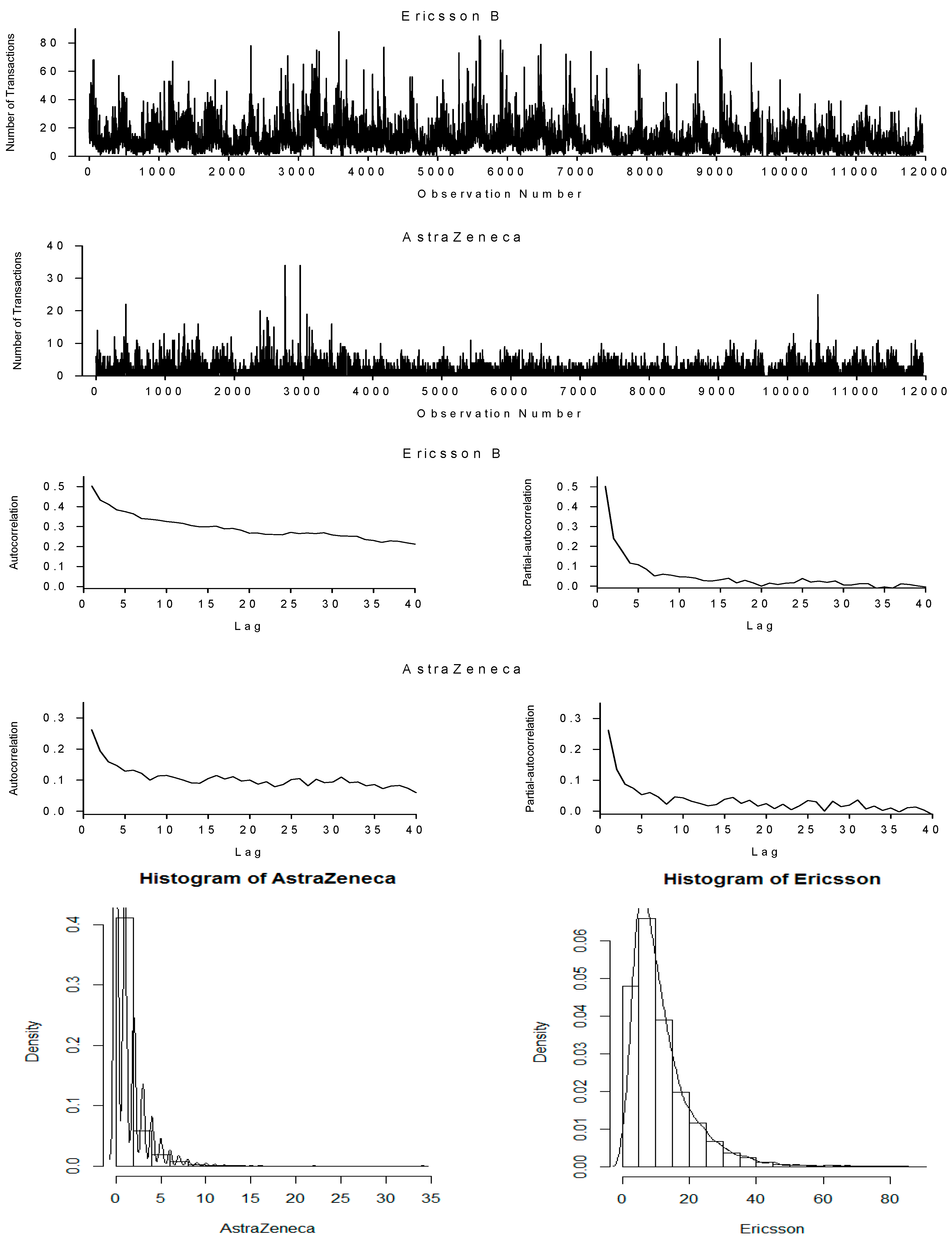
5. Data and Descriptive

In this paper, we use the same data set used by Quoreshi (2014). The reason for this is that we introduce Quasi-Maximum Likelihood Method, which has not been considered in the study and the studies on count data earlier due to unknown underlying distribution. We intend to employ this method on the same data set and replicate the previous study to compare with results emerged from employing this method. Quoreshi (2014) has downloaded the tick-by-tick data for Ericsson B and AstraZeneca from the Ecovision system and the data are later filtered to generate transaction data which are counts. The stocks are frequently traded and have the highest turnovers at the Stockholmsbörsen. The two stock series are collected for the period 5 November–12 December 2002. Due to a technical problem in downloading data there are no data for 12 November in the time series and the first captured minutes of 5 December is 1037. Since we are interested in capturing the number of ordinary transactions, we have deleted all trading before 0935 (trading opens at 0930) and after 1714 (order book closes at 1720). The transactions in the first few minutes are subject to a different trading mechanism while there is practically no trading after 1714. The data are aggregated into one minute intervals of time. For high frequency data, researchers usually use one, two, five, or ten minute intervals of time and the choice is rather arbitrary. There are altogether 11,960 observations for both the Ericsson B and AstraZeneca series. The series together with their autocorrelation and partial-autocorrelation functions and histograms are exhibited in Figure 1. There are frequent zero frequencies in both series, especially in the AstraZeneca series, and hence the application of count data modeling is called for. The counts in both series fluctuate around their means which is an indication of mean reverting processes. The autocorrelation functions for both series suggest fractional integration which implies long memory. The histograms exhibit the distribution of counts and the possible empirical densities of the counts. Even with relatively large sample size, the distributions appear far from being normally distributed. On the other hand, the distributions appear to be similar to Poisson distribution; both variances are greater than their respective means (Figure 1). Hence, there is no scope for employing known distributions.

6. Empirical Results

CLS, FGLS, and 2SQML are employed for estimation with lag length of 70 following the suggestions of Brännäs and Quoreshi (2010). It is to be noted that the AIC and SBIC criteria are not applicable in the context of long memory (Brännäs and Quoreshi 2010; Quoreshi 2014), which is also supported by the Monte Carlo Experiment. The results of the empirical studies are presented in

Table 4. CLS, FGLS, and 2SQML estimates for Ericsson and AstraZeneca.

	Ericsson			AstraZeneca
	CLS	FGLS	ML	CLS	FGLS	ML
$\widehat{d}$	0.324	0.324	0.324	0.204	0.204	0.204
(s.e)	0.008	0.008	0.008	0.012	0.012	0.011
$\widehat{\lambda }$	2.625	2.625	2.625	0.507	0.507	0.507
(s.e)	0.091	0.092	0.088	0.027	0.027	0.026
Var	-	-	54.722	-	-	3.303
(s.e.)	-	-	1.809	-	-	0.151
AIC	48,010.160	48,010.160	48,010.160	14,433.565	14,433.565	14,433.565
SBIC	48,534.802	48,534.802	48,534.802	14,958.207	14,958.207	14,958.207
QLB100	335.111	335.111	335.111	235.586	235.586	235.587
QLB200	422.191	422.191	422.191	352.309	352.309	352.309
MSE	54.722	54.722	54.722	3.303	3.303	3.303

. Empirically, we find evidence for long memory property ($\widehat{d}$< 0.5) for both Ericsson B and AstraZeneca series (see Table 4). The series for both AstraZeneca and Ericsson has mean reversion property and is covariance stationary. The findings suggest that the impact of macroeconomic news or rumors in one point of time has a persistence impact on future transactions. It may be recalled that news disseminated through formal channels which may have impact on overall stock markets and specifically on a particular stock is termed macroeconomic news, such as news on interest rates or unemployment statistics for a country which may influence all stocks. Rumors are information that spread through unofficial channels yet is related to macroeconomic news or a particular stock. For AstraZeneca, we find that CLS perform best while 2SQML performs better than FGLS in terms of eliminating serial correlation. Considering the standard error of the parameters ($\widehat{\lambda }, \widehat{d}$), we find that 2SQML performs best among the three estimators, while CLS performs better than FGLS. For Ericsson B, we find that 2SQML performs best in terms of both eliminating serial correlations and minimum standard error for the parameters. All other corresponding estimates turn out equal up to 3 decimals estimated by the three estimators.

7. Concluding Remarks

This paper introduces Quasi-Maximum Likelihood Estimation of Integer-Valued Long Memory Model for unknown underlying distribution and the estimation procedures for QML have been discussed. The paper compares the 2SQML estimator with FGLS and CLS. In a Monte Carlo experiment, it is found that the 2SQML, FGLS, and CLS estimators perform equally well in terms of eliminating serial correlation. The empirical study suggests that CLS performs best for AstraZeneca, while 2SQML performs best for Ericsson B in terms of eliminating serial correlations. However, the 2SQML estimator performs better than both the CLS and FGLS in terms of minimum standard error for estimates of the parameters for both Ericsson B and AstraZeneca, although CLS perform best followed by 2SQML in the simulation study. Note that the data in the simulation study is equidispersed since the data is generated from the Poisson distribution, while the data for the empirical study is overdispersed. The results of the study collectively may indicate that 2SQML estimator is relatively more efficient compared to CLS and FGLS for overdispersed data. The empirical results suggest that both series have long memory properties, which implies that the impact of macroeconomic news or rumors in one point of time has a persistence impact on future transactions.

References

1. Al-Osh, M. A., and Aus A. Alzaid. 1987. First Order Integer-Valued Autoregressive INAR(1)) Process. Journal of Time Series Analysis 8: 261–75. [Google Scholar] [CrossRef]
2. Al-Osh, M. A., and Aus A. Alzaid. 1988. Integer-Valued Moving Average (INMA) Process. Statistical Papers 29: 281–300. [Google Scholar] [CrossRef]
3. Andersen, Torben G., Tim Bollerslev, Francis X. Diebold, and Heiko Ebens. 2001. The distribution of realizedstockreturn volatility. Journal of Financial Economics 61: 43–76. [Google Scholar] [CrossRef]
4. Bhardwaj, Geetesh, and Norman R. Swanson. 2005. An Empirical Investigation of the Usefulness of ARFIMA Models for Predicting Macroeconomic and Financial Time Series. Journal of Econometrics 131: 539–78. [Google Scholar] [CrossRef]
5. Box, George E. P., and David A. Pierce. 1970. Distribution of Residual Autocorrelations in Autoregressive-Integrated Moving Average Time Series Models. Journal of the American Statistical Association 65: 1509–26. [Google Scholar] [CrossRef]
6. Brännäs, Kurt, and Eva Brännäs. 2004. Conditional Variance in Count Data Regression. Communication in Statistics; Theory and Methods 33: 2745–58. [Google Scholar] [CrossRef]
7. Brännäs, Kurt, and Andreia Hall. 2001. Estimation in Integer-Valued Moving Average Models. Applied Stochastic Models in Business and Industry 17: 277–91. [Google Scholar] [CrossRef]
8. Brännäs, Kurt, and A. M. M. Shahiduzzaman Quoreshi. 2010. Integer-Valued Moving Average Modelling of the Number of Transactions in Stocks. Applied Financial Economics 20: 129–440. [Google Scholar] [CrossRef]
9. Demsetz, Harold. 1968. The Cost of Transacting. Quarterly Journal of Economics 82: 33–53. [Google Scholar] [CrossRef]
10. Diamond, Douglas W., and Robert E. Verrecchia. 1987. Constraints on Short-Selling and Asset Price Adjustments to Private Information. Journal of Financial Economics 18: 277–311. [Google Scholar] [CrossRef]
11. Drost, Feike C., Ramon Van den Akker, and Bas J. M. Werker. 2009. Efficient estimation of auto-regression parameters and innovation distributions for semiparametric integer-valued AR(p) models. Journal of the Royal Statistical Society: Series B (Statistical Methodology) 71: 467–85. [Google Scholar] [CrossRef]
12. Easley, David, and Maureen O’hara. 1992. Time and the Process of Security Price Adjustment. Journal of Finance 47: 905–27. [Google Scholar] [CrossRef]
13. Engle, Robert F. 2000. The Econometrics of Ultra-High Frequency Data. Econometrica 68: 1–22. [Google Scholar] [CrossRef]
14. Gourieroux, Christian, Alain Monfort, and Alain Trognon. 1984. Pseudo Maximum Likelihood Methods: Application to Poisson Models. Econometrica 52: 701–20. [Google Scholar] [CrossRef]
15. Granger, Clive W. J. 1980. Long Memory Relationships and the Aggregation of Dynamic Models. Journal of Econometrics 14: 227–38. [Google Scholar] [CrossRef]
16. Granger, Clive W. J., and Zhuanxin Ding. 1996. Varieties of Long Memory Models. Journal of Econometrics 73: 61–77. [Google Scholar] [CrossRef]
17. Granger, Clive W. J., and Roselyne Joyeux. 1980. An Introduction to Long-Memory Time Series Models and Fractional Differencing. Journal of Time Series Analysis 1: 15–29. [Google Scholar] [CrossRef]
18. Heinen, Andréas, and Erick Rengifo. 2003. Multivariate Modelling of Time Series Count Data: An Autoregressive Conditional Poisson Model. CORE Discussion Paper 2003/25. Louvain-la-Neuve: Université Catholique de Louvain. [Google Scholar]
19. Hosking, J. R. M. 1981. Fractional Differencing. Biometrika 68: 165–76. [Google Scholar] [CrossRef]
20. Hurst, Harold Edwin. 1951. Long-Term Storage Capacity of Reservoirs. Transactions of the American Society of Civil Engineers 116: 770–808. [Google Scholar]
21. Hurst, Harold Edwin. 1956. Methods of Using Long-Term Storage in Reservoirs. Proceedings of the Institute of Civil Engineers 1: 519–43. [Google Scholar] [CrossRef]
22. Jacobs, Patricia A., and Peter A. W. Lewis. 1978a. Discrete Time Series Generalized by Mixtures I: Correlational and Runs Properties. Journal of the Royal Statistical Society B 40: 94–105. [Google Scholar]
23. Jacobs, Patricia A., and Peter A. W. Lewis. 1978b. Discrete Time Series Generalized by Mixtures II: Asymptotic Properties. Journal of the Royal Statistical Society B 40: 222–28. [Google Scholar]
24. Jacobs, Patricia A., and Peter A. W. Lewis. 1983. Stationary Discrete Autoregressive Moving Average Time Series Generated by Mixtures. Journal of Time Series Analysis 4: 19–36. [Google Scholar] [CrossRef]
25. Ljung, Greta M., and George E. P. Box. 1978. On a Measure of a Lack of Fit in Time Series Models. Biometrika 65: 297–303. [Google Scholar] [CrossRef]
26. Mandelbrot, Benoit B., and John W. van Ness. 1968. Fractional Brownian Motions, Fractional Noises and Applications. SIAM Review 10: 422–37. [Google Scholar] [CrossRef]
27. McKenzie, Ed. 1986. Autoregressive Moving-Average Processes with Negative Binomial and Geometric Marginal Distributions. Advances in Applied Probability 18: 679–705. [Google Scholar] [CrossRef]
28. Quoreshi, A. M. M. Shahiduzzaman. 2006. Bivariate Time Series Modelling of Financial Count Data. Communications in Statistics: Theory and Methods 35: 1343–58. [Google Scholar] [CrossRef]
29. Quoreshi, A. M. M. Shahiduzzaman. 2008. A vector integer-valued moving average model for high frequency financial count data. Economics Letters 101: 258–61. [Google Scholar] [CrossRef]
30. Quoreshi, A. M. M. Shahiduzzaman. 2014. A Long Memory, Count Data, Time Series Model for Financial Application. Quantitative Finance 14: 2225–35. [Google Scholar] [CrossRef]
31. Quoreshi, A. M. M. Shahiduzzaman. 2017. A bivariate integer-valued long-memory model for high-frequency financial count data. Communications in Statistics: Theory and Methods 46. [Google Scholar] [CrossRef]
32. Ristic, Miroslav M., Yuvraj Sunecher, Naushad Ali Mamode Khan, and Vandna Jowaheer. 2018. A GQL-based Inference in non-stationary BINMA(1) Time Series. TEST, 1–13. [Google Scholar] [CrossRef]
33. Rydberg, Tina Hviid, and Neil Shephard. 1999. BIN Models for Trade-by-Trade Data. Modelling the Number of Trades in a Fixed Interval of Time. Working Paper Series W23. Oxford: Nuffield College. [Google Scholar]
34. Smith, Jeremy, Nick Taylor, and Sanjay Yadav. 1996. Comparing the bias and Misspecification in ARFIMA models. Journal of Time Series Analysis 18: 507–27. [Google Scholar] [CrossRef]
35. Sunecher, Yuvraj, Naushad Mamode Khan, and Vandna Jowaheer. 2018. BINMA(1) Model with COM-Poisson Innovations: Estimation and Application. Communication in Statistics: Simulation and Computation, 1–22. [Google Scholar] [CrossRef]
36. Weiss, Andrew A. 1986. Asymptotic theory for ARCH models: Estimation and testing. Econometric Theory 2: 107–31. [Google Scholar] [CrossRef]
37. Working, Holbrook. 1953. Futures Trading and Hedging. American Economic Review 43: 314–43. [Google Scholar]
Figure 1. The time series of Ericsson B (mean 11.73 and variance 84.86) and AstraZeneca (mean 1.33 and variance 3.75) and their autocorrelation and partial-autocorrelation functions.
Jrfm 12 00074 g001