Defined Contribution Pension Plans: Who Has Seen the Risk?

Abstract

The trend towards eliminating defined benefit (DB) pension plans in favour of defined contribution (DC) plans implies that increasing numbers of pension plan participants will bear the risk that final realized portfolio values may be insufficient to fund desired retirement cash flows. We compare the outcomes of various asset allocation strategies for a typical DC plan investor. The strategies considered include constant proportion, linear glide path, and optimal dynamic (multi-period) time consistent quadratic shortfall approaches. The last of these is based on a double exponential jump diffusion model. We determine the parameters of the model using monthly US data over a 90-year sample period. We carry out tests in a synthetic market which is based on the same jump diffusion model and also using bootstrap resampling of historical data. The probability that portfolio values at retirement will be insufficient to provide adequate retirement incomes is relatively high, unless DC investors adopt optimal allocation strategies and raise typical contribution rates. This suggests there is a looming crisis in DC plans, which requires educating DC plan holders in terms of realistic expectations, required contributions, and optimal asset allocation strategies.

1. Introduction

Defined benefit (DB) pension plans can be high risk liabilities for both private and public sector organizations. To de-risk balance sheets, many employers have been gradually converting to defined contribution (DC) plans. This trend has been particularly strong in Australia and the US: as of 2017, 87% of pension assets in Australia were in DC plans, while the corresponding figure for the US was 60%. In contrast, in countries such as the UK, Canada, and Japan, pension plan assets were still predominantly in DB plans.1 Of course, considering just the percentage of assets in DC plans at a point in time can hide the underlying trend. For example, about 95% of Canadian pension assets were in DB plans as of 2017. However, Gougeon (2009) points out that the number of DC plan participants in Canada almost doubled between 1991 and 2006, while the number of DB plan participants shrank by about 4% over the same period.

Under a DC plan, the employee and employer contribute to a retirement savings account, which is usually tax-advantaged. In some cases, the employee is able to select from a list of investments (e.g., stock and bond index funds) which have been approved by the employer. However, in terms of the important decisions about asset allocation, the employee is typically left up to her own devices.

Although DC plans are desirable from the employers’ point of view, the retirement savings risk has simply been transferred to those who are perhaps least able to manage it. Many studies have confirmed that the average retail investor is very poor at managing investment portfolios (e.g., Barber and Odean (2013)). A typical DC plan investor will accumulate savings for thirty or more years, followed by a decumulation phase of perhaps twenty years. As a result, inefficiencies in asset allocation, even if small in annual terms, can have very large cumulative effects over a typical long-term retirement savings investment horizon.

Target date funds (TDFs) have become a popular means of providing an autopilot asset allocation strategy. The prototypical TDF uses a high allocation to equities during the early years of DC savings. The stock allocation is decreased, and the portfolio becomes more weighted towards bonds, as the retirement date nears. The transition from high to low equity allocations is pre-determined by means of a glide path strategy. In the US, TDFs are Qualified Default Investment Alternatives, implying that the assets of employees enrolled in an employer-managed DC plan can be invested in a TDF by default.2 Holt (2018) indicates that total assets in US TDFs at the end of September 2018 were almost $1.19 trillion, and notes that “given their role as the default investment in many defined contribution retirement plans, investors can expect to see assets in target-date funds continue to rise over the long run”.3 This reflects the tendency of many DC plan participants to stick with the default option that is presented to them. This has been noted in the US context by Madrian and Shea (2001) and Choi et al. (2002) amongst several others, and by other authors in various other countries as well.4 An implication of investors’ choosing default options is that default asset allocations will have a strong effect on the accumulation of savings over time (Dobrescu et al., 2018). Choi et al. (2002) note that

Sophisticated employers should choose their plan defaults carefully, since these defaults will strongly influence the retirement preparation of their employees. Policymakers should also recognize the role of defaults, since policymakers can facilitate, with laws and regulations, the socially optimal use of defaults.

(Choi et al. 2002, p. 104)

However, several studies have reported that TDFs do not appear to outperform simpler constant proportion strategies (Arnott et al., 2013; Basu et al., 2011; Esch and Michaud, 2014; Estrada, 2014; Forsyth and Vetzal, 2019). Clearly, constant proportion strategies which have a significant allocation to equities could result in a wide range of terminal wealth at the end of the accumulation period. The fact that TDFs are not superior to such strategies indicates that TDFs are not a panacea for DC plan investors.

Our objective in this article is to describe realistic outcomes for a typical DC plan investor who contributes a fixed (real) amount per year to an account containing two possible assets, a low risk bond fund and an equity index fund, over a lengthy (30 year) accumulation period, and who follows one of three different asset allocation strategies. The first two of these strategies are often available as default options in US DC plans, these being a constant proportion strategy and a linear glide path, which approximately mimics a prototypical TDF. These strategies are both deterministic since the asset allocation between the bond and equity funds is pre-specified and does not change as a result of realized investment returns. The third strategy is an optimal dynamic (multi-period) quadratic shortfall (QS) strategy. While such a strategy is not (to our knowledge) currently available for DC plan investors, it is an interesting extension to consider since it is adaptive, i.e., the asset allocation is a function of the prevailing state of the investment portfolio and the time remaining until anticipated retirement. Our investigation of this strategy allows us to draw conclusions about the extent to which adaptive strategies could potentially improve savings outcomes compared to the types of strategies that are currently popular default options. Unlike the constant proportion and glide path strategies, the QS strategy relies on a parametric model for the equity index. Our implementation models the real (inflation-adjusted) stock index as following a double exponential jump diffusion model (Kou and Wang, 2004), which incorporates the risk of sudden market crashes.5 The parameters of the jump diffusion model are estimated by fitting to nine decades of US market data.

The QS strategy is computed by numerically solving a Hamilton–Jacobi–Bellman (HJB) equation (Dang and Forsyth, 2014). It is interesting to note that the QS strategy, which is naturally time consistent, is equivalent to the pre-commitment multi-period mean-variance (MV) strategy, in the sense that both objective functions lead to the same optimal controls. This can be proven based on the embedding technique (Li and Ng, 2000; Zhou and Li, 2000). Our numerical approach allows us to impose realistic no-leverage constraints. This avoids the impractical situation of a highly leveraged portfolio, which often results for unconstrained pre-commitment MV optimal strategies (Lioui and Poncet, 2016)6.

As a benchmark case, we consider a constant proportion strategy involving the two assets listed above: a risk-free bond index and a risky stock index. The portfolio is annually rebalanced. The weights on the two assets are chosen to achieve a target expected level of real wealth at the end of the savings period. We then compare this strategy with a glide path and an optimal QS strategy, both of which are constrained to have the same expected value of final wealth as the constant proportion strategy. The glide path and constant proportion asset allocation strategies can be considered to be typical of many DC plan holders. The optimal QS strategy is effectively a best case scenario, in terms of reducing the probability of shortfall (over a wide range of the terminal wealth distribution) compared to glide path or constant proportion strategies (Forsyth and Vetzal, 2017b); Forsyth and Vetzal (2019).

We compare these strategies in a synthetic market, in which the equity price process is assumed to follow a jump diffusion with constant parameters (i.e., the average historical parameters). We also carry out tests using bootstrap resampling with actual historical data (Cogneau and Zakalmouline, 2013; Dichtl et al., 2016).

We make several assumptions which allow us to convert a desired final salary replacement ratio into a target real portfolio value after a 30-year contribution period. Our base case example assumes a target real final salary replacement ratio of 50%, a combined annual employee-employer contribution of 20% of real salary, and investments in short-term risk-free government bonds and a value-weighted equity index.

Our two main findings are as follows:

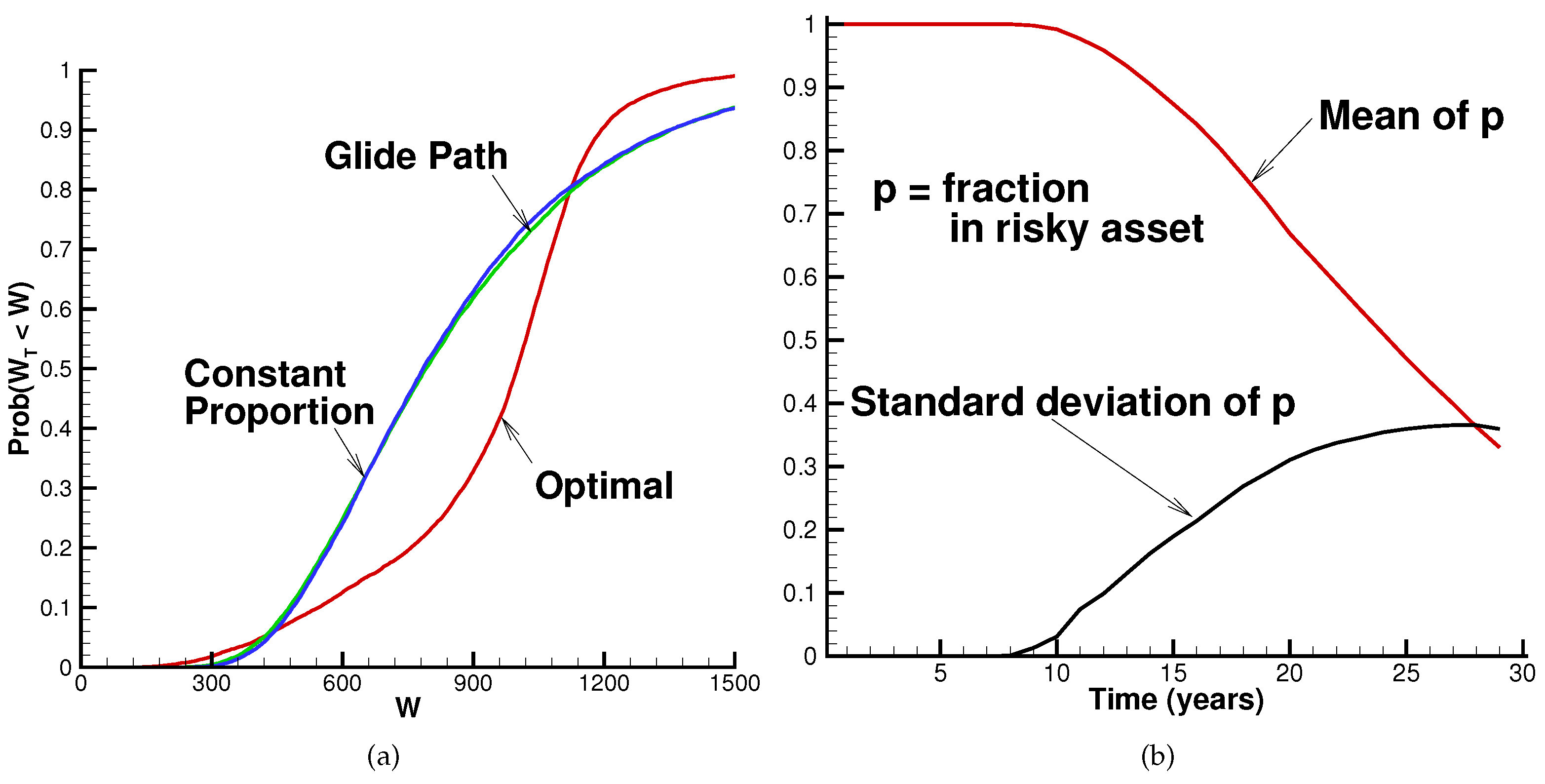
• With typical glide path or constant proportion strategies, there is an unacceptably large probability of shortfall in terms of meeting the target final wealth goal.
• Even with an optimal dynamic QS asset allocation strategy, there is still a fairly high probability of shortfall. This shortfall probability can be reduced to what we view as a reasonable level by increasing the total contribution rate or reducing the replacement ratio, compared to the base case. Another possibility is to substitute an equal-weighted equity index for the value-weighted index, but this may not work in practice due to higher costs associated with equal-weighted indexes, which are not recognized in our model.

Our results suggest that most DC plan holders are unlikely to be able to maintain their desired standard of living upon retirement. In our opinion, the true risks of DC plans have not been communicated in realistic terms to plan participants. It seems that this situation can be improved only by simultaneously lowering expectations, increasing savings rates, and improving asset allocation strategies. We emphasize that while, in principle, an optimal QS strategy could be offered as an option to DC plan members by a financial intermediary, and this would give those who selected it improved odds of achieving sufficient levels of retirement savings to maintain their desired living standards in retirement, by itself this is unlikely to be enough. It will also be necessary to raise savings rates and reduce expectations about living standards during retirement.

A possible criticism of our findings is based on the fact that our computations use the past 90 years of US market data. Some would argue that real market returns going forward will be lower than historically observed values. However, this would only lead to worse results, so it could be argued that our conclusions should be even more pessimistic.

2. Formulation

We focus exclusively on a simple context with just two assets available in the financial market, namely a risky asset and a risk-free asset. In practice, the risky asset would be a broad market index fund. An investor saves for retirement at time T. The amounts that this investor’s portfolio contains of the risky and risk-free assets at time t are denoted by $S_t$ and $B_t$, respectively. The investor’s total wealth from the portfolio (i.e., the total value of the portfolio) at t is $W_t=S_t+B_t$. The fraction of total wealth invested in the risky asset is $p_t=S_t/W_t$. The investment period runs from the inception time $t=0$ to the horizon date $t=T$. There is a set of $M+1$ pre-determined action times denoted by $\mathcal{T}$,

$$\mathcal{T}\equiv \left\{t_0=0\le t_1\le \cdots \le t_M=T\right\}.$$

(1)

At the horizon date $t_M=T$, the portfolio is liquidated. At each action time $t_i\in {\mathcal{T}}_1=\mathcal{T}\backslash \left\{t_M\right\}$ (i.e., each action time prior to T), (i) an amount of cash $q_i$ is contributed to the portfolio and then (ii) the portfolio is rebalanced.7

Let the instant before action time $t_i$ be $t_i^{-}=t_i-ϵ$, where $ϵ\to 0^{+}$. Similarly, the instant after $t_i$ is denoted by $t_i^{+}=t_i+ϵ$. To simplify notation, let $S_i^{+}=S_{t_i^{+}}$, $S_i^{-}=S_{t_i^{-}}$, $B_i^{+}=B_{t_i^{+}}$, $B_i^{-}=B_{t_i^{-}}$, $W_i^{+}=W_{t_i^{+}}$, and $W_i^{-}=W_{t_i^{-}}$. Similarly, let $p_{t_i^{+}}=p_i$.

Between action times (i.e., $t\notin \mathcal{T}$), the value of the investor’s portfolio will fluctuate in accordance with changes in the unit prices of the two assets. We assume a constant risk-free rate r, so that the evolution of the amount invested in the risk-free asset is

$$d{B}_t=r{B}_{t}dt,t\notin \mathcal{T}.$$

(2)

The dynamics of the changes in the amount invested in the risky asset between action times are given by the jump diffusion process

$$\frac{d{S}_t}{S_{t^{-}}}=\left(\mu -\lambda \kappa \right)dt+\sigma dZ+d\left(\sum _{i=1}^{{\pi }_t}\left({\xi }_i-1\right)\right),t\notin \mathcal{T},$$

(3)

where $\mu$ is the (uncompensated) drift rate, $\sigma$ is the volatility, $dZ$ is the increment of a Wiener process, ${\pi }_t$ is a Poisson process with intensity $\lambda$, and $\xi$ denotes the random jump multiplier. When a jump occurs, $S_t=\xi S_{t^{-}}$, and $\kappa =E[\xi -1]$ where $E[·]$ is the expectation operator. We assume that ${\xi }_i$ are i.i.d. positive random variables characterized by a double exponential distribution (Kou and Wang, 2004). Given that a jump occurs, $p_{up}$ is the probability of an upward jump and $\left(1-p_{up}\right)$ is the probability of a downward jump. The density function $f(y=log\xi )$ is then

$$f\left(y\right)=p_{up}{\eta }_1{e}^{-{\eta }_{1}y}{\mathbf{1}}_{y\ge 0}+(1-p_{up}){\eta }_2{e}^{{\eta }_{2}y}{\mathbf{1}}_{y<0}.$$

(4)

We do not permit short sales of the risky asset, and we impose an upper bound on the use of leverage, i.e., borrowed funds obtained through short sales of the risk-free asset. This means that there is an upper bound on the weight that the investor can place on the risky asset, which we denote by $L_{max}$. In other words, $0\le p_i\le L_{max}$ for all action times $t_i\in {\mathcal{T}}_1$. Generally, with a DC account, it is reasonable to specify $L_{max}=1$, ruling out the use of any leverage. Since the value of the risky asset follows the jump diffusion (3), if we allow leverage by setting $L_{max}>1$, the investor can become insolvent.8 We add the further constraint that, if the investor becomes insolvent at any time, then trading stops and all positions in the risky asset are liquidated.9 In insolvency, debt accumulates until it is (possibly) eliminated by cash contributions. We emphasize that insolvency can only occur if leverage is allowed, i.e., $L_{max}>1$.

2.1. Deterministic Glide Paths

TDFs generally use a deterministic glide path, where the asset allocation depends only on time. In our case, this would imply $p_i=p\left(t\right)$. One case is a linear glide path, with

$$p_i=p_{max}+\frac{t_i\times \left(p_{min}-p_{max}\right)}{T},$$

(5)

where $p_{max}$ and $p_{min}$ are parameters. Note also that a constant proportion strategy can be viewed as a deterministic glide path with $p=\mathrm{const}.$ for all action times $t_i\in {\mathcal{T}}_1$.

Between action times, the amounts the investor has in the risk-free and risky assets follow the processes (2) and (3), respectively. Recalling that $q_i$ is a cash contribution, at action times prior to the horizon date (i.e., $t_i\in {\mathcal{T}}_1$), we have

$$\begin{array}{cc}\hfill W_i^{+}& =S_i^{-}+B_i^{-}+q_i,\hfill \\ \hfill S_i^{+}& =p_i{W}_i^{+},\hfill \\ \hfill B_i^{+}& =(1-p_i)W_i^{+}.\hfill \end{array}$$

(6)

In the case of deterministic glide paths, closed form recursive expressions for the mean and variance of terminal wealth $W_T$ are developed in Forsyth and Vetzal (2019). The cumulative distribution function (CDF) for $W_T$ is computed using a Monte Carlo method. In our numerical tests below, we compare all strategies by fixing expected terminal wealth. Since we have closed form expressions for the mean, we determine the glide path parameters using a Newton iteration in order to enforce this condition.10

2.2. Adaptive Strategies

In contrast to deterministic strategies where the asset allocation depends only on time, adaptive strategies allow the asset allocation to depend on the prevailing state of the investment portfolio. Since we search for the optimal controls over all portfolios with the same wealth after cash injection ($W_i^{+}$), this means that $p_i=p_i(W_i^{+},t_i^{+})$. With an adaptive strategy, it can be optimal to withdraw cash from the portfolio (Cui et al., 2014; Dang and Forsyth, 2016). We denote this optimal cash withdrawal as $c_i\equiv c(W_i^{-}+q_i,t_i)$. Since we only allow cash withdrawals, $c_i\ge 0$. The control at action time $t_i$ now consists of the pair $(p_i,c_i)$, i.e., after withdrawing $c_i$ from the portfolio, rebalance so that the fraction invested in the risky asset is $p_i$.

For explanatory purposes, let us consider first consider a dynamic (multi-period) MV criterion with a specified desired value of $E\left[W_T\right]=W_d$. The problem to be solved can be stated as

$$\begin{array}{cc}\hfill \underset{\left\{\left(p_0,c_0\right),\cdots ,\left(p_{M-1},c_{M-1}\right)\right\}}{min}& \mathrm{Var}\left[W_T\right]=E\left[W_T^2\right]-W_d^2,\hfill \\ \hfill \mathrm{subject}\mathrm{to}& \left\{\begin{array}{c}\mathrm{At}\mathrm{horizon}T:E\left[W_T=S_T+B_T\right]=W_d,\hfill \\ \mathrm{Between}\mathrm{action}\mathrm{times}t\notin \mathcal{T}:(B_t,S_t)\mathrm{follow}\mathrm{processes}\left(2),\right(3),\hfill \\ \mathrm{At}\mathrm{action}\mathrm{times}t\in {\mathcal{T}}_1:\hfill \\ W_i^{+}=S_i^{-}+B_i^{-}+q_i-c_i,\hfill \\ S_i^{+}=p_i{W}_i^{+},B_i^{+}=W_i^{+}-S_i^{+},\hfill \\ p_i=p_i\left(W_i^{+},t\right),0\le p_i\le L_{max},\hfill \\ c_i=c_i\left(W_i^{-}+q_i,t\right)c_i\ge 0.\hfill \end{array}\right..\hfill \end{array}$$

(7)

A criticism of the pre-commitment MV problem (7) is that it is time inconsistent. In other words, the investor has an incentive to deviate from the strategy computed at time zero (Basak and Chabakauri, 2010). However, in order to solve problem (7), we can use the embedding technique (Li and Ng, 2000; Zhou and Li, 2000). Consider a control set

$$P=\left\{\left(p_i\left(W_i^{+},t_i^{+}\right),c_i\left(W_i^{-}+q_i,t_i\right)\right),i=0,\cdots ,M-1\right\}.$$

Informally, if $P^{*}$ is an optimal control for problem (7), then there exists a $W^{*}$ such that $P^{*}$ is also the optimal control for the following problem:

$$\begin{array}{cc}\hfill \underset{\left\{\left(p_0,c_0\right),\cdots ,\left(p_{M-1},c_{M-1}\right)\right\}}{min}& E\left[{\left(W^{*}-W_T\right)}^2\right],\hfill \\ \hfill \mathrm{subject}\mathrm{to}& \left\{\begin{array}{c}\mathrm{At}\mathrm{horizon}T:E\left[W_T=S_T+B_T\right]=W_d,\hfill \\ \mathrm{Between}\mathrm{action}\mathrm{times}t\notin \mathcal{T}:(B_t,S_t)\mathrm{follow}\mathrm{processes}\left(2),\right(3),\hfill \\ \mathrm{At}\mathrm{action}\mathrm{times}t\in {\mathcal{T}}_1:\hfill \\ W_i^{+}=S_i^{-}+B_i^{-}+q_i-c_i,\hfill \\ S_i^{+}=p_i{W}_i^{+},B_i^{+}=W_i^{+}-S_i^{+},\hfill \\ p_i=p_i\left(W_i^{+},t\right),0\le p_i\le L_{max},\hfill \\ c_i=c_i\left(W_i^{-}+q_i,t\right)c_i\ge 0.\hfill \end{array}\right..\hfill \end{array}$$

(8)

Problem (8) can be solved using dynamic programming methods.11

As noted above, it is optimal to withdraw cash from the portfolio under some conditions (Cui et al., 2012; Dang and Forsyth, 2016). Let

$$Q_{\ell }=\sum _{j=\ell +1}^{j=M-1}{e}^{-r\left(t_j-t_{\ell }\right)}{q}_j$$

(9)

be the discounted planned future contributions to the DC account at time $t_{\ell }$. If

$$\left(W_i^{-}+q_i\right)>W^{*}{e}^{-r(T-t_i)}-Q_i,$$

(10)

then the optimal strategy is to

(i)

withdraw cash $c_i=W_i^{-}+q_i-\left(W^{*}{e}^{-r(T-t_i)}-Q_i\right)$ from the portfolio; and

(ii)

invest the remainder $\left(W^{*}{e}^{-r(T-t_i)}-Q_i\right)$ in the risk-free asset.

This is optimal because in this case $E\left[{\left(W^{*}-W_T\right)}^2\right]=0$, which is the minimum of problem (8).

We refer to any cash withdrawn from the portfolio as surplus cash in the following. For the sake of discussion, we will assume that surplus cash is invested in the risk-free asset, but does not contribute to the calculation of the mean and variance of terminal wealth.

Allowing cash withdrawals prevents penalization of wealth paths such that $W_T>W^{*}$, which can result in forcing the optimal strategy to lose money if market gains are good, which is clearly an undesirable outcome (Cui et al., 2012; Dang and Forsyth, 2016). We remark that in practice, this withdrawal can be virtual, i.e., any amount of wealth satisfying equation (10) is simply invested in the risk-free asset, and and the surplus cash is not taken into account when computing the optimal fraction to invest in equities. See Dang and Forsyth (2016) for more detail on this. In fact, if we use continuous rebalancing, then the optimal strategy is such that Equation (10) is never satisfied (Vigna, 2014). In the discrete rebalancing case, the generation of surplus cash is a low probability event.

This target-based approach of problem (8) provides a reasonable objective on its own (Menoncin and Vigna, 2017; Vigna, 2014, 2017). Solving (8) minimizes quadratic shortfall (QS) with respect to $W^{*}$, so we will refer to the resulting strategy as the QS optimal strategy below. However, this becomes even more compelling when we recall that the solution is also pre-commitment MV efficient. The solution then simultaneously minimizes two risk measures: variance around the desired $E\left[W_T\right]$ and QS with respect to $W^{*}$, as seen at time zero.

We emphasize that the fact that the pre-commitment MV policy is time inconsistent is irrelevant since we take the point of view that we are seeking the QS optimal control, from problem (8). Since the QS problem (8) can be solved using dynamic programming, the controls are trivially time consistent. The fact that the QS problem gives rise to time consistent controls, whereas the MV problem (7) is time inconsistent, is due to the fact that we fix $W^{*}$ for the QS problem, for all time. At time zero, the MV problem controls and the QS problem controls are the same for $W^{*}$ computed at time zero. At later times, this correspondence holds only if we allow $W^{*}$ to change as a function of time. However, using a fixed $W^{*}$ is intuitively reasonable for DC pension plan saving (Menoncin and Vigna, 2017; Vigna, 2014).

We note that there are techniques for forcing a time consistent constraint for the MV problem (7) (Bjork and Murgoci, 2010, 2014; Bjork et al., 2014; Wang and Forsyth, 2011). However, we prefer the target based QS approach since it is relatively easy to communicate to end user investors (Menoncin and Vigna, 2017; Vigna, 2014). In addition, forcing the time consistent constraint can have result in non-intuitive strategies with strange features (Bensoussan et al., 2019; Wang and Forsyth, 2011).

We formulate problem (8) as the solution of a nonlinear Hamilton–Jacobi–Bellman (HJB) partial integro differential equation. See Dang and Forsyth (2014) for details concerning the numerical solution. Given an arbitrary value of $W^{*}$, we can solve problem (8) for the optimal control, which we denote by $P^{*}\left(W^{*}\right)$. Given the optimal control, cumulative distribution functions are easily found using Monte Carlo simulation. However, we seek the solution to problem (7), which is expressed in terms of a specified expected value $E\left[W_T\right]=W_d$. We determine the value of $W^{*}$ for problem (8) which satisfies the constraint $E\left[W_T\right]=W_d$. We enforce this by a Newton iteration, whereby each function evaluation requires a solution of an HJB equation.

3. Data and Parameter Estimates

The underlying stochastic model outlined above in Equations (2), (3), and (4) involved a constant risk-free rate r for the bond component and a double exponential jump-diffusion for the equity component. Estimation of the parameters of these equations follows the methods described in Forsyth and Vetzal (2019). These procedures are summarized briefly here for convenience. Readers interested in additional details are referred to Forsyth and Vetzal (2019).

We use monthly US data obtained from the Center for Research in Security Prices (CRSP) for the period 1926:1 through 2015:12.12 Our base case uses the CRSP value-weighted total return index (which includes all distributions for all domestic equities trading on major US exchanges), along with the CRSP 3-month Treasury bill (T-bill) index. The original data are in nominal terms, but we convert them to real terms using the US CPI, also obtained from CRSP. We use real indexes since investors with long-term savings objectives such as funding retirement should concentrate on real (not nominal) wealth goals. For some tests, we use alternative underlying assets: the CRSP equal-weighted total return index (which invests the same amount in each component security, rather than weighting by market capitalization) and a 10-year US Treasury bond (T-bond) index.

Figure 1 provides plots of monthly real returns for the 3-month T-bill, 10-year T-bond, value-weighted total return, and equal-weighted total return indexes. For comparability, all four indexes are plotted with the same vertical axis scale. As expected, the two equity indexes exhibit much higher volatility, with occasional months having returns of large magnitude. This provides a measure of support to our modelling assumptions which assume a constant interest rate but a jump diffusion specification for the equity index. It is also interesting to observe that there was extremely high equity market volatility during the 1930s. By contrast, volatility during the period following the financial crisis that began in 2007 was comparatively mild.

Figure 2 graphs cumulative real returns for the four investment indexes. The vertical axis uses a logarithmic scale. This enhances visibility over time, as otherwise the dramatic growth in the equity indexes over the latter part of the sample obscures the behaviour of those indexes during the earlier periods and renders the behaviour of the two Treasury indexes all but invisible. All four indexes begin at a value of 100 at the start of 1926. The equal-weighted index ends up with the highest value. The historical outperformance of equal-weighting has been attributed to such portfolios having higher exposure to value, size, and market factors (Plyakha et al., 2014). It is also interesting to observe that the 10-year T-bond index had higher cumulative returns than the 3-month T-bill index, but that was entirely due to the post-1980 period: prior to then, the longer maturity T-bond index offered no cumulative advantage over the T-bill index.

Table 1. Annualized parameter estimates based on real monthly data from 1926:1 to 2015:12. These values originally appeared in Forsyth and Vetzal (2019) and are reproduced here for convenience. Parameters for the equity market indexes were estimated using the threshold technique of Cont and Mancini (2011). The average returns for the bond indexes were calculated as $log\left[B\right(T)/B(0\left)\right]/T$, where $B\left(t\right)$ denotes the index level at the time t.

Equity Market Index	$\mathit{\mu }$	$\mathit{\sigma }$	$\mathit{\lambda }$	${\mathit{p}}_{\mathit{up}}$	${\mathit{\eta }}_1$	${\mathit{\eta }}_2$
Value-weighted	0.0889	0.1477	0.3222	0.2759	4.4273	5.2613
Equal-weighted	0.1183	0.1663	0.4000	0.3333	3.6912	4.5409
Bond Market Index	Average Return
3-month T-bill	0.00827
10-year T-bond	0.02160

presents parameter estimates. A threshold method (Cont and Mancini, 2011) was used for the jump diffusion model. These parameter estimates were originally provided in Forsyth and Vetzal (2019), and are reproduced here for convenience. The estimates using the value-weighted equity market index imply an expected real annual return of close to 9%, about 3% lower than the corresponding value for the equal-weighted index. Of course, the price to be paid for this difference is higher risk. The equal-weighted index shows higher diffusive volatility ($\sigma$). Since jumps are expected to occur on average every $1/\lambda$ years, the equal-weighted index tends to have jumps a bit more often. Conditional on a jump occurring, it is much more likely to be a downward jump in each case. Average jump magnitudes are $1/{\eta }_1$ for upward jumps and $1/{\eta }_2$ for downward jumps, and these are both larger for the equal-weighted index. A similar comment applies to the standard deviation of the jump size since this is equal to the mean for the exponential distribution. Turning to the bond market indexes, Table 1 shows that the long run average real annual return for the 10-year T-bond index was just over 2%, while that for the shorter maturity index was around 80 basis points. Of course, these higher returns are accompanied by higher volatility, as indicated by the top two plots of Figure 1.

Robustness to Parameter Estimation

Our main purpose for calibrating the parameters for the stochastic processes (3) is to determine a control strategy (i.e., fraction in risky asset at rebalancing dates). Consequently, our concern is with the effect of calibration errors on the computed strategy, rather than minimizing fit errors in an econometric sense. In Forsyth and Vetzal (2017a) and in Dang and Forsyth (2016), an extensive study of the effect of parameter ambiguity is carried out. In particular, the parameters for stochastic process (3) were determined using maximum likelihood, and threshold techniques with various parameters. Robustness of the strategy (in the synthetic market) was tested by using Monte Carlo simulations with different parameters than were used in computing the optimal strategy. For example, the strategy was computed and stored, assuming parameters determined from the threshold strategy. Then, this strategy was tested using Monte Carlo simulations, in a synthetic market driven by a stochastic process with parameters determined using maximum likelihood. In other words, the parameters used to compute the strategy were misspecified. In all combinations of methods, the results were robust to this type of parameter misspecification.

However, the real test of our strategies is their performance on bootstrapped resampled tests. In the bootstrap tests, we make no assumptions about the stochastic process followed in the historical market. However, in all our bootstrap tests, the adaptive quadratic shortfall strategy (computed using the estimated market parameters) outperforms the glide path and constant proportion strategies.

4. Base Case Scenario

We consider an example where a DC plan member wants to generate retirement income (in real terms) of a specified fraction R of final salary. Studies have shown that earnings for a typical employee increase rapidly until the age of 35, then increase slowly thereafter, until a few years before retirement, and then decrease as fewer hours are worked in the transition to retirement (Cocco et al., 2005; Ruppert and Zanella, 2015). Given an initial real annual salary $I_0$, we assume that real annual income in year t before retirement is given by $I_t=e^{{\mu }_{I}t}{I}_0$. In other words, salary is expected to grow in real terms at a constant annual rate ${\mu }_I$. Upon retirement at time T, real annual salary is $e^{{\mu }_{I}T}{I}_0$. Our assumptions would be relevant to a 35 year old employee with stable employment, who intends to work full-time until the age of 65.

To determine the amount of real wealth required to fund this replacement income during retirement, we use the well-known 4% rule of Bengen (1994). Bengen examined historical data to determine the maximum real withdrawal rate that a retiree could safely use without exhausting her assets over a 35 year period. Bengen assumed that accumulated pension wealth was invested in a portfolio having half invested in stocks and half invested in intermediate-term US Treasury securities, and concluded that a 4% withdrawal rate (escalated by the rate of inflation) was quite safe.

Dang et al. (2017) recently revisited this rule. The problem was posed somewhat differently: the idea was to determine a real withdrawal rate such that half of the real wealth at the start of retirement remained after 20 years, with high probability. Rather than using fixed portfolio weights as in Bengen (1994), the portfolio was invested in stocks and bonds according to the QS optimal strategy described above. Dang et al. concluded that the 4% rule still held up well under the revised assumptions.

An obvious alternative way to generate retirement cash flows is to buy a lifetime annuity. However, in practice most retirees are not willing to do this, for a variety of reasons (MacDonald et al., 2013). In the current environment of low real interest rates, annuities provide rather low income, so the reluctance of retirees to use them is particularly unsurprising.

Consequently, we pose the pension accumulation problem as follows. The desired expected accumulated real wealth at retirement $W_d$ is

$$E\left[W_T\right]=W_d=\frac{R{e}^{{\mu }_{I}T}{I}_0}{w_r},$$

(11)

where R is the replacement ratio, $I_0$ is the initial salary, ${\mu }_I$ is the real salary escalation rate, T is the end of the accumulation period, and $w_r$ is the safe withdrawal rate. Recall that above we denoted the set of action times prior to T as ${\mathcal{T}}_1$. We assume that cash is contributed into the portfolio at time $t_i\in {\mathcal{T}}_1$. The initial cash contribution at $t_0$ is $F_c{I}_0$, where $F_c$ is the real contribution fraction. This contribution fraction represents the total amount contributed by both the employee and the employer to all retirement savings accounts, but excludes any government sponsored universal schemes (e.g., CPP in Canada, Social Security in the US). We also assume that these accounts are tax-advantaged, i.e., no tax is paid during the accumulation phase. At subsequent action times $t_i\in {\mathcal{T}}_1$ (i.e., after the initial contribution), the amount contributed is assumed to be $F_c{I}_0{e}^{{\mu }_i{t}_i}$.

Table 2. Data for base case scenario. Cash is injected into the portfolio at times $t=0,1,\cdots ,29$. Market parameters for the equity and bond indexes are provided in Table 1.

Initial salary $I_0$	$50,000
Salary escalation rate ${\mu }_I$	0.0127 (Bloom et al., 2014)
Contribution fraction $F_c$	0.20
Accumulation period T	30 years
Safe withdrawal rate $w_r$	0.04
Equity index	Value-weighted
Bond index	3-month T-bill
Investment strategies	Constant proportion, glide path, QS optimal
Rebalancing interval	1 year
Maximum leverage indicator $L_{max}$	1.0
If insolvent	Trading stops

summarizes the data for this base case scenario. As indicated in the table, we assume a replacement fraction of 50%, an initial salary of $50,000, and a real escalation rate of 1.27%.13 Combined contributions by the employee and employer to the retirement savings portfolio are 20% of real salary each year. For simplicity, these contributions are assumed to be made at the start of each year during a 30 year accumulation period. The safe withdrawal rate is assumed to be 4%, in line with Bengen (1994) and Dang et al. (2017). Applying these parameters to Equation (11), we find that the expected (real) desired terminal wealth $W_d$ is

$$E\left[W_T\right]=W_d=\frac{0.50}{0.04}\times \$50,000e^{.0127\times 30}\simeq \$915,000.$$

(12)

Note that the specification given in Equation (11) implies that decreasing the withdrawal rate $w_r$ has the same effect as increasing the replacement fraction R or the salary escalation rate ${\mu }_I$.

As indicated in Table 2, the retirement savings portfolio is invested in the value-weighted index and the 3-month T-bill index. Relevant parameters for these indexes are given in Table 1. We consider three alternative investment strategies:

• Constant proportion, i.e., $p=const$.
• Linear glide path, as in Equation (5).
• Time consistent QS optimal strategy, as described in Section 2.2. Recall that this strategy is also multi-period pre-commitment MV optimal.

Each of these strategies is rebalanced annually. We start with the constant proportion strategy, and determine the equity weight such that $E\left[W_T\right]=\$915,000$, assuming the market parameters given in Table 1 for the value-weighted equity index and the 3-month T-bill index. This turns out to be $0.5788$.14 We then turn to the linear glide path strategy. In this case, we specify $p_{max}=1.0$, and then determine that the value of $p_{min}=0.3066$ is needed to have $E\left[W_T\right]=\$915,000$. We proceed similarly for the QS optimal strategy given by the solution to problem (8). Imposing the leverage constraint $L_{max}=1.0$, we find by Newton iteration that the value of $W^{*}$ which results in $E\left[W_T\right]=\$915,000$ is $1,106,200. We compute and store the optimal control associated with this value of $W^{*}$ in order to test this strategy. Note that:

• When we change input parameters (e.g., invest in different assets, allow $L_{max}>1$, etc.), we may need to recompute the expected wealth target $E\left[W_T\right]=W_d$, the equity weight for the constant proportion strategy, the glide path parameters $(p_{max},p_{min})$, and the quadratic wealth target $W^{*}$ (along with the associated optimal control) in order to meet this target.
• The quadratic wealth target $W^{*}$ exceeds the target expected real terminal wealth $W_d=E\left[W_T\right]$. This is because the QS optimal strategy will de-risk if $W^{*}$ is attainable by investing only in the risk-free asset, so there is not much chance of exceeding this quadratic target by a significant amount. This implies that the average terminal wealth, factoring in paths where the accumulated savings does not ever reach $W^{*}$, must be lower than $W^{*}$.

We compare these three strategies using two different types of simulation tests. As an initial test, we assume that the stochastic environment described in Table 1 holds exactly. In other words, the level of the equity market index follows a double exponential jump diffusion with the parameters given in Table 1 and the bond market index is non-stochastic, with a constant risk-free interest rate as indicated in that table. We refer to this as a synthetic market. In such a market, we draw 160,000 Monte Carlo simulated paths and compute performance statistics. Note that these comparisons are based on a simulated environment that corresponds exactly to the environment used to formulate the strategies. As a second and more stringent test, we draw simulated paths by bootstrap resampling of the historical return data and compute the same performance statistics. We refer to this type of backtest as a historical market. This is a stricter test since it does not assume that the equity market follows a jump diffusion process or that the risk-free interest rate is constant over time, although those assumptions are still used to generate the strategies that are followed. A single resampled path is constructed by pasting together enough blocks of monthly historical return data to cover the investment horizon of 30 years. The sampling is done in blocks to account for possible serial dependence. The blocks are selected simultaneously from both the historical stock and bond market indexes, to incorporate possible correlations. The blocks are chosen randomly, with replacement. To avoid end issues, the historical data is wrapped around.15 To reduce the impact of a fixed blocksize and mitigate edge effects at each block end, we use the stationary block bootstrap (Patton et al., 2009; Politis and White, 2004) where the blocksize is sampled randomly from a geometric distribution with an expected value of $\widehat{b}$. In principle, the optimal expected blocksize can be estimated using an algorithm provided by Patton et al. (2009). As discussed in Forsyth and Vetzal (2019), this approach is not easily applied in our context. This is because the estimated optimal blocksizes for the different market indexes we consider (i.e., the value-weighted and equal-weighted US equity market indexes and the 3-month T-bill and 10-year T-bond indexes) vary considerably, ranging from about two months for the value-weighted stock index to more than four years for the T-bill index. Recall that we sample simultaneously from both a stock index and a bond index, so we must use the same blocksize for both indexes, and our strategies involve weighted combinations of two of these indexes that can change deterministically (glide path) and also randomly (QS optimal) along a simulation path. As a result, we report results for a range of expected blocksizes $\widehat{b}$, acknowledging that the choice of $\widehat{b}$ for our application is open to debate.

Table 3. Base case scenario results. Wealth units: thousands of dollars. Input data provided in Table 1 and Table 2. Synthetic market results computed using Monte Carlo simulations with 160,000 sample paths. Historical market results based on 10,000 bootstrap resampled paths using data from 1926:1 to 2015:12.

Strategy	Expected Value	Standard Deviation	$\mathit{Pr}({\mathit{W}}_{\mathit{T}}<700)$	$\mathit{Pr}({\mathit{W}}_{\mathit{T}}<800)$	Expected Surplus Cash
Synthetic Market
Constant proportion	915	519	0.39	0.51	NA
Glide path	915	519	0.39	0.51	NA
QS optimal	915	244	0.19	0.24	21
Historical Market (Expected blocksize $\widehat{b}=1$ year)
Constant proportion	876	402	0.38	0.51	NA
Glide path	872	398	0.39	0.52	NA
QS optimal	904	232	0.18	0.24	26
Historical Market (Expected blocksize $\widehat{b}=2$ years)
Constant proportion	869	376	0.38	0.51	NA
Glide path	866	372	0.39	0.52	NA
QS optimal	911	221	0.17	0.23	31
Historical Market (Expected blocksize $\widehat{b}=5$ years)
Constant proportion	862	349	0.37	0.50	NA
Glide path	861	347	0.38	0.51	NA
QS optimal	924	213	0.16	0.21	38

gives the results for the base case input data from Table 2. Consider first the synthetic market. By construction, all three strategies have the same expected value of real terminal wealth at the retirement date of 915 (units in the table are in thousands of dollars). The constant proportion and glide path strategies are effectively indistinguishable, having the same standard deviation of terminal wealth and the same probability of ending up with wealth below 700 or below 800. By contrast, the QS optimal strategy has much lower standard deviation or shortfall probability for those two levels of terminal wealth, by a factor of around two in each case. In addition, this strategy offers a small amount of expected surplus cash (this surplus is not applicable for the other two strategies). Turning to the historical market results for expected blocksizes of 1, 2, and 5 years, we reach generally similar conclusions. Of course, the expected values no longer are exactly equal to the target of 915, but the difference from this target is much lower for the QS optimal strategy. The constant proportion and glide path strategies are again quite comparable to each other, with the glide path having slightly lower expected value and standard deviation, but a bit higher shortfall probability (for the two values of $W_T$ considered). In all cases, the QS optimal strategy offers the best performance, with higher mean, lower standard deviation, and lower shortfall probability, as well as a modest amount of expected surplus cash.

Figure 3a shows the cumulative distributions for all three strategies in the historical market (expected blocksize of two years). The distributions for the constant proportion and glide path strategies are practically identical. Over the bulk of the distribution, the QS optimal strategy exhibits clearly better performance than the others. However, the QS optimal strategy performs a little worse than the alternatives in the extreme left tail.16 This happens because there can be paths where the equity market trends downward for a very large portion of the investment horizon. In such cases, all strategies do poorly, but the QS optimal strategy will remain fully invested in the equity market in an attempt to recover and meet the quadratic wealth target. The QS optimal strategy also underperforms in the extreme right tail of the distribution. This is because there are paths where the equity market trends strongly upward over most of the investment period. Once the quadratic wealth target is reached, however, the QS optimal strategy de-risks, shifting all investment into the low return bond market. It does not capitalize on the continued strong equity market performance. The other two strategies, by comparison, retain a large equity market exposure, leading to higher terminal wealth. However, we reiterate that, over most of the distribution, the QS optimal strategy provides better results.

Figure 3b depicts properties of the optimal control for the QS optimal strategy. This strategy invests entirely in the equity market for the first several years. The percentage invested in the risky asset subsequently trends downward on average over time. However, there is considerable variation: the standard deviation of the optimal control rises strongly over time, indicating that the allocation to equities is quite sensitive to realized investment returns.17

The historical market results given in Table 3 are somewhat encouraging for the QS optimal strategy. To formulate this strategy, recall that we assumed a double exponential jump diffusion model with known parameters for the equity market index and a constant risk-free interest rate. Our bootstrap resampled historical market tests make no such assumptions, yet deliver results that are fairly close to those observed in the synthetic market tests which maintain these assumptions. This indicates that the QS optimal strategy is quite robust to departures from these assumptions.

As an additional test of the robustness of the QS optimal strategy, we explore the effect of computing and storing the optimal control based on constant parameters from Table 1 but then allowing the synthetic equity market parameters to vary randomly in simulation tests. To be specific, we carry out Monte Carlo simulations where at each action time $t_i\in {\mathcal{T}}_1$ and along each stochastic path we select $(\mu ,\sigma )$ from a uniform distribution having mean equal to the corresponding values from Table 1. This set of $(\mu ,\sigma )$ is then used for the interval $(t_i,t_{i+1})$.

Table 4. Base case scenario results for the QS optimal strategy with random variation of market parameters $\mu$ and $\sigma$, Wealth units: thousands of dollars. Input data provided in Table 1 and Table 2, except as noted. Monte Carlo simulations with $(\mu ,\sigma )$ drawn from a uniform distribution with the indicated limits along each of 160,000 paths.

Market Parameters	Expected Value	Standard Deviation	$\mathit{Pr}({\mathit{W}}_{\mathit{T}}<700)$	$\mathit{Pr}({\mathit{W}}_{\mathit{T}}<800)$	Expected Surplus Cash
Synthetic market	915	244	0.19	0.24	21
$\mu \in [0.04889,0.01289]$	916	245	0.19	0.24	21
$\sigma \in [0.1077,0.1877]$	915	245	0.19	0.24	21

shows the results. The first row reproduces the values reported in Table 3 for this strategy in the synthetic market, while the remaining two rows provide results when $\mu$ and $\sigma$ are varied randomly within the given range. Table 4 indicates that only an estimate of the mean of the distribution of the market parameters $\mu$ and $\sigma$ is needed to compute an effective control strategy. This is consistent with the results in Ma and Forsyth (2016), where it is shown that including stochastic volatility effects results in negligible improvements in results for long-term (i.e., greater than ten years) investors.

Overall, then, for the base case data in Table 2, the QS optimal strategy appears to be fairly robust to parameter and model mis-specification. Moreover, this strategy clearly outperforms the constant proportion and glide path alternatives over most of the terminal wealth distribution. It provides about the same mean terminal wealth, but has considerably lower standard deviation and shortfall probability (for the two wealth levels considered in Table 3). However, even the QS optimal strategy delivers somewhat disappointing results in absolute terms. Recall that we are trying to achieve average real terminal wealth of $915,000. In the idealized synthetic market which conforms exactly to the modelling assumptions used to generate the controls for the QS optimal strategy, Table 3 shows that there is almost a 20% chance of ending up with real terminal wealth below $700,000, and about a 25% chance of ending up with less than $800,000. These shortfall probabilities do not change much under the conditions of the historical market backtests. Of course, these rather pessimistic results so far have only considered the base case data. In the following section, we investigate whether more promising results can be achieved under different assumptions.

5. Alternative Assumptions

The base case results in Section 4 relied on the input parameters given in Table 1 and Table 2, for the value-weighted equity and 3-month T-bill indexes. We now explore the effects of altering our assumptions about factors such as the contribution fraction, the salary escalation rate, the maximum amount of leverage permitted, the underlying indexes to be used, and the salary replacement ratio. We consider each of these in turn. For the most part, we only use the QS optimal strategy since it has been shown above to be generally superior to the constant proportion and glide path strategies.

5.1. Effect of Contribution Fraction

Our base case described by Table 2 assumed a total combined contribution by the employee and employer of $F_c=20\%$ of salary.

Table 5. Effect of varying contribution fraction $F_c$ for the QS optimal strategy. Wealth units: thousands of dollars. Input data provided in Table 1 and Table 2, except as noted. Synthetic market results computed using Monte Carlo simulations with 160,000 sample paths. Historical market results based on 10,000 bootstrap resampled paths using data from 1926:1 to 2015:12.

${\mathit{F}}_{\mathit{c}}$	Expected Value	Standard Deviation	$\mathit{Pr}({\mathit{W}}_{\mathit{T}}<700)$	$\mathit{Pr}({\mathit{W}}_{\mathit{T}}<800)$	Expected Surplus Cash
Synthetic Market
0.15	915	440	0.36	0.42	18
0.20	915	244	0.19	0.24	21
0.25	915	150	0.09	0.13	21
Historical Market (Expected blocksize $\widehat{b}=2$ years)
0.15	916	380	0.34	0.41	12
0.20	911	221	0.17	0.23	31
0.25	909	126	0.07	0.14	67

reports the effects of dropping this to 15% or increasing it to 25% for the QS optimal strategy. As is to be expected, the table shows that risk (measured either in terms of standard deviation or the reported shortfall probabilities) decreases significantly as $F_c$ rises. However, even in the case where 25% of the employee’s salary is contributed to the retirement savings plan, there is still almost a 15% chance that real terminal wealth is less than $800,000, considerably lower than the target of $915,000. A broader comparison of these cases is provided in Figure 4, which depicts the cumulative distributions of real terminal wealth. The cases where $F_c=20\%$ and $F_c=25\%$ appear quite comparable for values of $W_T\ge \$915,000$ over the plotted range, but the higher contribution fraction case appears to be much safer over a wide range below the target. The high savings rate leads to a notably increased amount of expected surplus cash. Along paths with strong equity market returns, the target can be reached relatively early, but the model assumes that savings continue each year (in this case at a high rate), so surplus cash can build up. The case where $F_c=15\%$ exhibits poor performance on the downside, but is somewhat better on the upside. With a low amount of money saved, more risk must be taken on in order to reach the target. Doing so works out very well if realized returns are strong, and quite poorly if they are not.

5.2. Effect of Salary Escalation Rate

We now examine the effect of changing the salary escalation rate ${\mu }_I$ from the base case value of 1.27% given in Table 2. Note that this will result in a different expected real wealth target $W_d$, based on Equation (11).

Table 6. Effect of varying salary escalation rate ${\mu }_I$ for the QS optimal strategy. Units for $W_d$: thousands of dollars. Remaining wealth values are normalized by $W_d$ for each case. Input data provided in Table 1 and Table 2, except as noted. Synthetic market results computed using Monte Carlo simulations with 160,000 sample paths. Historical market results based on 10,000 bootstrap resampled paths using data from 1926:1 to 2015:12.

${\mathit{\mu }}_{\mathit{I}}$	Wealth Target ${\mathit{W}}_{\mathit{d}}$	Expected Value $({\mathit{W}}_{\mathit{T}}/{\mathit{W}}_{\mathit{d}})$	Standard Deviation $({\mathit{W}}_{\mathit{T}}/{\mathit{W}}_{\mathit{d}})$	$\mathit{Pr}({\mathit{W}}_{\mathit{T}}/{\mathit{W}}_{\mathit{d}}<0.8)$	$\mathit{Pr}({\mathit{W}}_{\mathit{T}}/{\mathit{W}}_{\mathit{d}}<0.9)$	Expected Surplus Cash $(/{\mathit{W}}_{\mathit{d}})$
Synthetic Market
0.0175	1056	1.0	0.31	0.25	0.30	0.02
0.0127	915	1.0	0.27	0.20	0.25	0.02
0.0075	783	1.0	0.22	0.15	0.21	0.02
Historical Market (Expected blocksize $\widehat{b}=2$ years)
0.0175	1056	0.99	0.29	0.23	0.29	0.03
0.0127	915	0.97	0.24	0.18	0.25	0.03
0.0075	783	0.99	0.19	0.14	0.21	0.04

summarizes the results for both the synthetic market and the historical market, using the QS optimal control. For comparability, the table expresses the results in terms of $W_T/W_d$, i.e., real terminal wealth as a fraction of the expected wealth target. Obviously, a higher escalation rate leads to a higher final salary. Given a fixed salary replacement ratio, this translates into a higher expected value of terminal wealth $W_d$. For example, with ${\mu }_I=1.75\%,$ we have $W_d=\$1,056,000$ instead of $915,000 as in the base case. The results in Table 6 are quite similar in the synthetic and historical markets, on a case by case basis. For each set of tests, the standard deviation and shortfall probabilities show an increase with ${\mu }_I$. With a higher salary and a fixed contribution fraction, there will obviously be a higher amount of saving. Despite this, the associated higher real terminal wealth target results in a higher level of risk. This is borne out in Figure 5, which plots the cumulative distribution functions of normalized real terminal wealth $W_T/W_d$ for the various values of ${\mu }_I$. The highest salary escalation rate has the worst performance for low $W_T/W_d$, and the best performance for high $W_T/W_d$. Taking on more risk to reach the higher wealth target works out well if investment returns are favourable, and poorly if they are not. Conversely, the lowest value of ${\mu }_I$ results in the best performance if investment returns are weak, and the worst performance if they are not.

5.3. Effect of Leverage

All of the results presented thus far have specified $L_{max}=1$, as indicated in Table 2. We now consider increasing this to $L_{max}=1.5$, thereby allowing the use of 50% leverage.

Table 7. Effect of varying maximum leverage indicator $L_{max}$ for the QS optimal strategy. Wealth units: thousands of dollars. Input data provided in Table 1 and Table 2, except as noted. Synthetic market results computed using Monte Carlo simulations with 160,000 sample paths. Historical market results based on 10,000 bootstrap resampled paths using data from 1926:1 to 2015:12.

${\mathit{L}}_{max}$	Expected Value	Standard Deviation	$\mathit{Pr}({\mathit{W}}_{\mathit{T}}<700)$	$\mathit{Pr}({\mathit{W}}_{\mathit{T}}<800)$	Expected Surplus Cash
Synthetic Market
1.0	915	244	0.19	0.24	21
1.5	915	205	0.12	0.17	24
Historical Market (Expected blocksize $\widehat{b}=2$ years)
1.0	911	221	0.17	0.23	31
1.5	904	186	0.11	0.18	46

documents the results for the QS optimal strategy. It is interesting to observe that the risk measures shown (standard deviation of $W_T$ and the two shortfall probabilities) each indicate somewhat lower risk when the use of leverage is permitted. In one sense, this is obvious: relaxing a constraint cannot lead to worse performance. On the other hand, leverage is often not allowed since it is perceived to be “risky”. The issue here is what is meant by risk. We have defined it on the basis of the value of terminal wealth. Leverage constraints, however, are typically motivated by concerns that portfolio values during the accumulation period (not at the end of the period) will fluctuate excessively.

Figure 6a shows the cumulative distributions of real terminal wealth when leverage is allowed and when it is not. The cumulative distributions are fairly similar for high levels of terminal wealth. Over a wide range of wealth levels below the target of $915,000, the strategy which permits leverage performs better. However, in the extreme left tail of the distribution, it turns out to be worse to allow leverage. These very low wealth levels occur as a result of very poor equity market returns over most of the investment horizon. The QS optimal strategy continues to try to reach the quadratic wealth target, so it invests completely in the equity market to the extent possible. With continued poor returns, leverage in this case amounts to doubling down on a losing bet.

5.4. Long-Term Bond Index

All of the results presented thus far were based on the value-weighted equity index and the 3-month T-bill index. In this section, we explore the effects of substituting the 10-year T-bond index for the T-bill index. Recall from Table 1 that the long-term bond index had average annual real returns of 2.16%, about 1.3% higher than the T-bill index. Of course, these higher average returns are accompanied by higher volatility (Figure 1), but that is ignored when we formulate the QS optimal strategy since we assume constant interest rates.

Table 8. Results for the optimal QS strategy when the 10-year T-bond index is used instead of the 3-month T-bill index. Wealth units: thousands of dollars. Input data provided in Table 1 and Table 2, except as noted. Synthetic market results computed using Monte Carlo simulations with 160,000 sample paths. Historical market results based on 10,000 bootstrap resampled paths using data from 1926:1 to 2015:12.

Strategy	Expected Value	Standard Deviation	$\mathit{Pr}({\mathit{W}}_{\mathit{T}}<700)$	$\mathit{Pr}({\mathit{W}}_{\mathit{T}}<800)$	Expected Surplus Cash
Synthetic Market
Constant proportion	915	437	0.34	0.47	NA
Glide path	915	438	0.34	0.48	NA
QS optimal	915	222	0.16	0.21	19
Historical Market (Expected blocksize $\widehat{b}=2$ years)
Constant proportion	900	374	0.34	0.47	NA
Glide path	897	376	0.34	0.48	NA
QS optimal	881	201	0.17	0.26	67

shows results for the constant proportion, linear glide path, and QS optimal strategies when the 10-year T-bond index is used in lieu of the 3-month T-bill index. The general pattern in Table 8 is similar to that seen earlier in Table 3. The QS optimal approach achieves roughly the same expected real terminal wealth, but takes on considerably lower risk compared to the other two strategies, as measured by standard deviation of $W_T$ or either of the two shortfall probabilities considered. Comparing the results from Table 3 and Table 8, we observe that the standard deviation and shortfall probabilities for each strategy are a little lower in the synthetic market when the 10-year T-bond index is used. This also holds in the historical market for the constant proportion and glide path strategies, but is not the case for the QS optimal strategy in terms of the shortfall probabilities. For example, the probability of real terminal wealth being lower than $800,000 is 23% if the 3-month T-bill index is used, but 26% when the 10-year T-bond index is used. The overall conclusion, however, is that replacing the 3-month T-bill index by the 10-year T-bond index does not make much difference. This picture is reinforced by comparing the cumulative distributions of real terminal wealth shown in Figure 7 based on the 10-year T-bond index with those shown previously in Figure 3a for the 3-month T-bill index.

5.5. Equal-Weighted Equity Index

As shown above in Figure 2, an equal-weighted equity index has historically outperformed the value-weighted equity index that has been used for all results to this point. We now consider the impact of replacing the value-weighted index by its equal-weighted counterpart. Note that the bond index used here is the 3-month T-bill index.

Table 9. Results when the equal-weighted equity index is used instead of the value-weighted equity index. Wealth units: thousands of dollars. Input data provided in Table 1 and Table 2, except as noted. Synthetic market results computed using Monte Carlo simulations with 160,000 sample paths. Historical market results based on 10,000 bootstrap resampled paths using data from 1926:1 to 2015:12.

Strategy	Expected Value	Standard Deviation	$\mathit{Pr}({\mathit{W}}_{\mathit{T}}<700)$	$\mathit{Pr}({\mathit{W}}_{\mathit{T}}<800)$	Expected Surplus Cash
Synthetic Market
Constant proportion	915	546	0.38	0.51	NA
Glide path	915	553	0.39	0.52	NA
QS optimal	915	185	0.11	0.16	44
Historical Market (Expected blocksize $\widehat{b}=1$ year)
Constant proportion	837	327	0.39	0.54	NA
Glide path	831	319	0.39	0.55	NA
QS optimal	904	162	0.10	0.16	49
Historical Market (Expected blocksize $\widehat{b}=2$ years)
Constant proportion	827	293	0.38	.54	NA
Glide path	820	283	0.38	0.55	NA
QS optimal	915	139	0.07	0.13	51
Historical Market (Expected blocksize $\widehat{b}=5$ years)
Constant proportion	815	248	0.36	0.53	NA
Glide path	808	242	0.37	0.55	NA
QS optimal	932	115	0.04	0.10	54

provides the results. Whether in the idealized synthetic market or the backtest historical market, the QS optimal strategy clearly outperforms the constant proportion and glide path alternatives by the criteria given in the table. In the synthetic market, the QS optimal strategy achieves the same $E\left[W_T\right]$ with dramatically lower standard deviation of $W_T$ and shortfall probability, along with the possibility of a modest amount of surplus cash. The same general conclusions apply in the historical market, although it is worth noting that the average real terminal wealth for the other strategies is somewhat lower for all expected blocksizes considered. Comparing the results in Table 9 for the equal-weighted equity index with those reported above in Table 3 for the value-weighted index, it can be seen that the shortfall probabilities are now considerably lower for the QS optimal strategy, but almost unchanged for the other strategies. The standard deviation of $W_T$, however, is substantially lower for all of the strategies.

Figure 8 plots the cumulative distributions of real terminal wealth in both the synthetic and the historical markets. In both cases, the distributions for the glide path and constant proportion strategies are virtually indistinguishable. Figure 8a indicates that the QS optimal strategy outperforms over a wide range of terminal wealth values in the synthetic market, although it does perform worse in the tails of the distribution. As mentioned earlier, this is due to two features of the strategy: (i) it automatically de-risks once the quadratic wealth target is achievable by investing only in the bond index (so it does not take advantage of continued strong equity market performance afterwards on paths where that happens); and (ii) it continually tries to reach the quadratic wealth target by using maximum equity market exposure (and this gamble for resurrection fails on paths where the equity market has persistently poor performance). The same comments apply to the historical market shown in Figure 8b, but it is worth noting that the underperformance of the QS optimal strategy in the tails is considerably reduced here compared to the synthetic market.

5.6. Effect of Replacement Ratio

All of the results provided to here assume a replacement ratio $R=50\%$ of final real salary, in accordance with Table 2. We now explore the effects of lowering this to 40% and increasing it to 60%. For each case, we determine the desired expected real wealth target by using Equation (11).

Table 10. QS optimal results with varying salary replacement ratios R. Units for $W_d$: thousands of dollars. Remaining wealth values are normalized by $W_d$ for each case. Input data provided in Table 1 and Table 2, except as noted. Synthetic market results computed using Monte Carlo simulations with 160,000 sample paths. Historical market results based on 10,000 bootstrap resampled paths using data from 1926:1 to 2015:12.

R	Wealth Target ${\mathit{W}}_{\mathit{d}}$	Expected Value $({\mathit{W}}_{\mathit{T}}/{\mathit{W}}_{\mathit{d}})$	Standard Deviation $({\mathit{W}}_{\mathit{T}}/{\mathit{W}}_{\mathit{d}})$	$\mathit{Pr}({\mathit{W}}_{\mathit{T}}/{\mathit{W}}_{\mathit{d}}<0.8)$	$\mathit{Pr}({\mathit{W}}_{\mathit{T}}/{\mathit{W}}_{\mathit{d}}<0.9)$	Expected Surplus Cash $(/{\mathit{W}}_{\mathit{d}})$
Synthetic Market
0.4	732	1.0	0.16	0.10	0.15	0.02
0.5	915	1.0	0.27	0.20	0.25	0.02
0.6	1098	1.0	0.37	0.31	0.36	0.02
Historical Market (Expected blocksize $\widehat{b}=2$ years)
0.4	732	.99	0.15	0.09	0.17	0.0
0.5	915	.97	0.24	0.18	0.25	0.03
0.6	1098	1.0	0.35	0.30	0.35	0.02

shows the results. Decreasing R to 40% reduces the expected wealth target $W_d$ to $732,000 from $915,000, while raising R to 60% increases $W_d$ to $1,098,000. The remaining wealth values in the table are normalized by $W_d$. Whether we consider the synthetic or the historical market, it is clear that increasing R requires taking on more risk, as measured by either the standard deviation or the shortfall probabilities. This is borne out in the cumulative distribution plots of normalized terminal real wealth provided in Figure 9. The synthetic market results in Figure 9a clearly indicate that the QS optimal strategy performs better for the lowest value of R. Recall that the strategy attempts to come as close as possible to $W_d$ (normalized to 1 for this plot), and the cumulative distribution when $R=40\%$ shows relatively low probability of normalized real wealth being much above or below 1. For the highest replacement ratio ($R=60\%$), there is a substantial chance of being either significantly below or above 1. This is because the strategy must take on more risk in order to attain the higher expected wealth target. Of course, the base case with $R=50\%$ lies in between these other two cases. The results for the historical market shown in Figure 9b are generally similar, though the differences across the range of values of R are somewhat less pronounced.

5.7. Summary Regarding Alternative Assumptions

Section 5.1, Section 5.2, Section 5.3, Section 5.4, Section 5.5 and Section 5.6 above provided detailed results concerning the effects of

• varying the accumulation fraction $F_c$, i.e., the investor saves $F_c{I}_0{e}^{{\mu }_I{t}_i}$ at each rebalancing date;
• varying the real salary escalation rate ${\mu }_I$;
• use of leverage;
• alternative bond index: use of a 10 year T-bond index instead of a 3 month T-bill index;
• alternative stock index: use of an equal-weighted equity index instead of a value-weighted index; and
• varying the replacement ratio R.

Table 11. Comparison of shortfall probabilities. Results are normalized by $W_d$ for each case. Input data provided in Table 1 and Table 2, except as noted. Historical market results based on 10,000 bootstrap resampled paths using data from 1926:1 to 2015:12 with expected blocksize $\widehat{b}=2$ years.

Case	$\mathit{Pr}({\mathit{W}}_{\mathit{T}}/{\mathit{W}}_{\mathit{d}}<0.8)$	$\mathit{Pr}({\mathit{W}}_{\mathit{T}}/{\mathit{W}}_{\mathit{d}}<0.9)$
Base Case, Table 2
Constant proportion	0.43	0.54
Glide path	0.43	0.54
QS optimal	0.18	0.25
QS Optimal
Contribution Fraction
$F_c=0.25$	0.09	0.17
$F_c=0.15$	0.37	0.43
Salary Escalation Rate
${\mu }_I=0.0175$	0.23	0.29
${\mu }_I=0.0075$	0.14	0.21
Leverage
$L_{max}=1.5$	0.13	0.19
Alternative Bond Index
10-year T-bond	0.19	0.28
Alternative Stock Index
Equal-weighted	0.09	0.16
Replacement Ratio
$R=0.4$	0.09	0.17
$R=0.6$	0.30	0.35

summarizes the results of various strategies in terms of probability of shortfall with respect to the desired wealth goal $W_d$. These results were all obtained using bootstrap resampling (i.e., for the historical market) with an expected blocksize of two years.

It is interesting to note that the results for the Base Case, constant proportion strategy (contribution rate 20%) are worse than the results for the QS optimal strategy, $F_c=0.15$ (contribution rate 15%), at least in terms of the two points of the cumulative distribution function listed in the table. In other words, the shortfall increase with a constant proportion strategy compared to the quadratic shortfall strategy can be interpreted as losing 5% of lifetime salary, which is very significant. However, this comparison does not take into account the entire cumulative distribution function. In general, constant proportion strategies are superior to quadratic shortfall policies in the extreme left tail of the distribution. However, the improvement over quadratic shortfall is very small, with a very low probability.

As a filter to determine an acceptable combination of DC plan parameters and investment strategies, suppose we specify that there should be at least a 90% probability of achieving at least 80% of the desired expected wealth goal $W_d$. Based on attempting to achieve the final target expected real wealth for the base case (see Table 2) and applying this filter, we can see that the shortfall probabilities using standard strategies (constant proportion or glide path) are unacceptably high. Using the QS optimal strategy leads to a substantial reduction in these shortfall probabilities, but still not to the desirable range of less than 10%.

From Equation (11), it is clear that the case with $R=0.6$ and $w_r=4\%$ leads to the same expected wealth target as specifying $R=0.5$ and $w_r=3.3\%$. Table 11 therefore indicates that, if we assume that the safe (real) withdrawal rate is 3.3% and the replacement ratio is 50%, the probability of shortfall is quite high even if the QS optimal strategy is followed.

Assuming we use the QS optimal allocation strategy, we are then forced to take other actions to attempt to reduce the shortfall probability. Increasing the contribution rate to $25\%$ of annual salary meets our criterion, but this might be difficult to implement in terms of agreement from employees and employers. Decreasing the replacement ratio ($40\%$ of final salary) also achieves the shortfall objective. We note that many institutions effectively do this by targeting a final career average salary replacement ratio (instead of a final salary replacement ratio).

Finally, the use of the alternative equal-weighted equity index also achieves the shortfall probability target. As noted earlier, this type of index has historically outperformed its value-weighted counterpart owing to higher exposure to value, size, and market factors (Plyakha et al., 2014). In effect, the equal-weighted portfolio is a smart beta portfolio, with a long track record. However, equal-weighted portfolios have higher costs, which have not been factored in to our analysis. This suggests that there may be a market opportunity for a low cost synthetic ETF which tracks the equal-weighted index.

6. Conclusions

Typical default strategies available to DC plan members include target date funds (i.e., glide path) and balanced funds (constant proportion). Both of these strategies have high probabilities of shortfall and large standard deviations of real terminal wealth.

We define an acceptable probability of success as a $90\%$ probability of achieving $80\%$ of the real desired terminal wealth goal. QS optimal strategies reduce the probability of shortfall significantly, compared to the ubiquitous glide path and balanced portfolio strategies, but not to within an acceptable range.

Assuming an optimal QS strategy, acceptable probabilities of shortfall can be obtained by

• reducing the final salary target replacement ratio ($40\%$ or less);
• increasing the total (employee and employer) contribution rate to $25\%$ per year;
• using alternative stock investment indices, such as an equal-weighted index. The backtests of an equal-weighted index perform well, but it is not clear that this will persist in the future. In addition, we have not factored in the additional costs of this type of index.

Our main conclusion is that current practices in DC plans with typical target benefits and default investment strategies have unacceptably high probabilities of shortfall. This has major ramifications for the many organizations which are shifting to DC plans.

Our results are based on the past 90 years of US market data. It is possible to argue that future market returns will be lower than observed in the past. The implication of such an assumption is that the probability of success for a DC investor would be even lower than we have reported here. In this case, the situation for DC plan investors would be even more dire than we suggest.

References

1. Arnott, Robert D., Katrina F. Sherrerd, and Lilian Wu. 2013. The glidepath illusion and potential solutions. The Journal of Retirement 1: 13–28. [Google Scholar] [CrossRef]
2. Barber, Brad M., and Terrance Odean. 2013. The behavior of individual investors. In Handbook of Economics and Finance. Edited by George Constantinides, Milton Harris and Rene Stulz. Amsterdam: Elsevier, chp. 22. pp. 1533–69. [Google Scholar]
3. Basak, Suleyman, and Georgy Chabakauri. 2010. Dynamic mean-variance asset allocation. Review of Financial Studies 23: 2970–3016. [Google Scholar] [CrossRef]
4. Basu, Anup K., Alistair Byrne, and Michael E. Drew. 2011. Dynamic lifecycle strategies for target date retirement funds. Journal of Portfolio Management 37: 83–96. [Google Scholar] [CrossRef]
5. Bengen, William. 1994. Determining withdrawal rates using historical data. Journal of Financial Planning 7: 171–180. [Google Scholar]
6. Bensoussan, Alain, Kwok Chuen Wong, and Sheung Chi Phillip Yam. 2019. A paradox in time-consistency in the mean-variance problem? Finance and Stochastics 23: 173–207. [Google Scholar] [CrossRef]
7. Björk, Tomas, and Agatha Murgoci. 2010. A General Theory of Markovian Time Inconsistent Stochastic Control Problems. SSRN 1694759. Rochester: Social Science Research Network. [Google Scholar]
8. Björk, Tomas, and Agatha Murgoci. 2014. A theory of Markovian time inconsisent stochastic control in discrete time. Finance and Stochastics 18: 545–92. [Google Scholar] [CrossRef]
9. Björk, Tomas, Agatha Murgoci, and Xun Yu Zhou. 2014. Mean-variance portfolio optimization with state-dependent risk aversion. Mathematical Finance 24: 1–24. [Google Scholar] [CrossRef]
10. Bloom, David E., David Canning, and Michael Moore. 2014. Optimal retirement with increasing longevity. Scandinavian Journal of Economics 116: 838–58. [Google Scholar] [CrossRef]
11. Choi, James J., David Laibson, Brigitte C. Madrian, and Andrew Metrick. 2002. Defined contribution pensions: Plan rules, participant choices, and the path of least resistance. Tax Policy and the Economy 16: 67–113. [Google Scholar] [CrossRef]
12. Cocco, João F., Franciso J. Goems, and Pascal J. Maenhout. 2005. Consumption and portfolio choice over the life cycle. Review of Financial Studies 18: 491–533. [Google Scholar] [CrossRef]
13. Cogneau, Phillipe, and Valereiy Zakamouline. 2013. Block bootstrap methods and the choice of stocks for the long run. Quantitative Finance 13: 1443–57. [Google Scholar] [CrossRef]
14. Cont, Rama, and Cecilia Mancini. 2011. Nonparametric tests for pathwise properties of semimartingales. Bernoulli 17: 781–813. [Google Scholar] [CrossRef]
15. Cui, Xiangyu, Jianjun Gao, Xun Li, and Duan Li. 2014. Optimal multi-period mean variance policy under no-shorting constraint. European Journal of Operational Research 234: 459–68. [Google Scholar] [CrossRef]
16. Cui, Xiangyu, Duan Li, Shouyang Wang, and Shushang Zhu. 2012. Better than dynamic mean-variance: Time inconsistency and free cash flow stream. Mathematical Finance 22: 346–78. [Google Scholar] [CrossRef]
17. Dang, Duy-Minh, and Peter A. Forsyth. 2016. Better than pre-commitment mean-variance portfolio allocation strategies: A semi-self-financing Hamilton–Jacobi–Bellman equation approach. European Journal of Operational Research 250: 827–41. [Google Scholar] [CrossRef]
18. Dang, Duy-Minh, Peter A. Forsyth, and Kenneth R. Vetzal. 2017. The 4% strategy revisited: A pre-commitment optimal mean-variance approach to wealth management data. Quantitative Finance 17: 335–51. [Google Scholar] [CrossRef]
19. Dang, Duy-Minh, and Peter A. Forsyth. 2014. Continuous time mean-variance optimal portfolio allocation under jump diffusion: A numerical impulse control approach. Numerical Methods for Partial Differential Equations 30: 664–98. [Google Scholar] [CrossRef]
20. Dang, Duy-Minh, Peter A. Forsyth, and Yuying Li. 2016. Convergence of the embedded mean-variance optimal points with discrete sampling. Numerische Mathematik 132: 271–302. [Google Scholar] [CrossRef]
21. Dichtl, Hubert, Wolfgang Drobetz, and Martin Wambach. 2016. Testing rebalancing strategies for stock-bond portfolos across different asset allocations. Applied Economics 48: 772–88. [Google Scholar] [CrossRef]
22. Dobrescu, Loretti I., Xiaodong Fan, Hazel Bateman, Ben R. Newell, A. Ortmann, and Susan Thorp. 2018. Retirement savings: A tale of decisions and defaults. Economic Journal 128: 1047–94. [Google Scholar] [CrossRef]
23. Esch, David N., and Robert O. Michaud. 2014. The False Promise Of Target Date Funds. Working Paper. Boston: New Frontier Advisors, LLC. [Google Scholar]
24. Estrada, Javier. 2014. The glidepath illusion: An international perspective. Journal of Portfolio Management 40: 52–64. [Google Scholar] [CrossRef]
25. Forsyth, Peter A., and Kenneth R. Vetzal. 2017a. Dynamic mean variance asset allocation: Tests for robustness. International Journal of Financial Engineering 4: 1750021. [Google Scholar] [CrossRef]
26. Forsyth, Peter A., and Kenneth R. Vetzal. 2017b. Robust asset allocation for long-term target-based investing. International Journal of Theoretical and Applied Finance 20: 1750017. [Google Scholar] [CrossRef]
27. Forsyth, Peter A., and Kenneth R. Vetzal. 2019. Optimal asset allocation for retirement saving: Deterministic vs. time consistent adaptive strategies. Applied Mathematical Finance. forthcoming. [Google Scholar] [CrossRef]
28. Gougeon, Phillipe. 2009. Shifting pensions. Statistics Canada: Perspectives on Labour and Income 10: 16–23. [Google Scholar]
29. Hedesström, Ted M., Henrik Svedsäter, and Tommy Gärling. 2004. Identifying heuristic choice rules in the Swedish premium pension scheme. Journal of Behavioral Finance 5: 32–42. [Google Scholar] [CrossRef]
30. Holt, Jeff. 2018. Target-Date Funds Keep Growing In Popularity. Available online: www.morningstar.com/videos/889903/targetdate-funds-keep-growing-in-popularity.html (accessed on 9 April 2019).
31. Kou, Steven, and Hui Wang. 2004. Option pricing under a double exponential jump diffusion model. Management Science 50: 1178–92. [Google Scholar] [CrossRef]
32. Li, Duan, and Wan-Lung Ng. 2000. Optimal dynamic portfolio selection: Multiperiod mean-variance formulation. Mathematical Finance 10: 387–406. [Google Scholar] [CrossRef]
33. Lioui, Abrahan, and Patrice Poncet. 2016. Understanding dynamic mean variance asset allocation. European Journal of Operational Research 254: 320–37. [Google Scholar] [CrossRef]
34. Ma, Kai, and Peter A. Forsyth. 2016. Numerical solution of the Hamilton–Jacobi–Bellman formulation for continuous time mean variance asset allocation under stochastic volatility. Journal of Computational Finance 20: 1–37. [Google Scholar] [CrossRef]
35. MacDonald, Bonnie-Jean, Bruce Jones, Richaard J. Morrison, Robert L. Brown, and Mary Hardy. 2013. Research and reality: A literature review on drawing down retirement savings. North American Actuarial Journal 17: 181–215. [Google Scholar] [CrossRef]
36. Madrian, Brigitte C., and Dennis F. Shea. 2001. The power of suggestion: Inertia in 401(k) participation and savings behavior. Quarterly Journal of Economics 116: 1149–87. [Google Scholar] [CrossRef]
37. Menoncin, Francesco, and Elena Vigna. 2017. Mean-variance target based optimisation for defined contribution pension schemes in a stochastic framework. Insurance: Mathematics and Economics 76: 172–84. [Google Scholar] [CrossRef]
38. O’Connell, Allison. 2009. Kiwisaver: A model scheme? Social Policy Journal of New Zealand 36: 130–41. [Google Scholar]
39. Patton, Andrew, Dimitris Politis, and Halbert White. 2009. Correction to: Automatic block-length selection for the dependent bootstrap. Econometric Reviews 28: 372–375. [Google Scholar] [CrossRef]
40. Pielichata, Paulina. 2018. Europeans seeing funds as solution to DC dilemma. Pensions & Investments, March 19. [Google Scholar]
41. Plyakha, Yuliya, Raman Uppal, and Grigory Vilkov. 2014. Equal or Value Weighting? Implications For Asset-Pricing Tests. Working Paper. Lille, Nice and Paris: EDHEC Business School. [Google Scholar]
42. Politis, Dimitris, and Halbert White. 2004. Automatic block-length selection for the dependent bootstrap. Econometric Reviews 23: 53–70. [Google Scholar] [CrossRef]
43. Ruppert, Peter, and Giulio Zanella. 2015. Revisiting wage, earnings, and hours profiles. Journal of Monetary Economics 72: 114–30. [Google Scholar] [CrossRef]
44. Tse, Shu-Tong, Peter A. Forsyth, and Yuying Li. 2014. Preservation of scalarization optimal points in the embedding technique for continuous time mean variance optimization. SIAM Journal on Control and Optimization 52: 1527–46. [Google Scholar] [CrossRef]
45. Vigna, Elena. 2014. On efficiency of mean-variance based portfolio selection in defined contribution pension schemes. Quantitative Finance 14: 237–58. [Google Scholar] [CrossRef]
46. Vigna, Elena. 2017. Tail Optimality And Preferences Consistency For Intertemporal Optimization Problems. Working Paper No. 502. Collegio Carlo Alberto: Università Degli Studi di Torino. [Google Scholar]
47. Wang, Jian, and Peter A. Forsyth. 2011. Continuous time mean variance asset allocation: A time-consistent strategy. European Journal of Operational Research 209: 184–201. [Google Scholar] [CrossRef]
48. Zhou, Xun Yu, and Duan Li. 2000. Continuous-time mean-variance portfolio selection: A stochastic LQ framework. Applied Mathematics and Optimization 42: 19–33. [Google Scholar] [CrossRef]
1.
Statistics from the Thinking Ahead Institute’s “Global Pension Assets Study 2018”. Available online: www.thinkingaheadinstitute.org/-/media/Pdf/TAI/Research-Ideas/GPAS-2018.pdf.
2.
In other words, the employee must explicitly decide to opt out of a TDF if she desires a different asset allocation strategy.
3.
Although our focus in this article is on the US setting, we note that TDFs are now being marketed in various parts of Europe, in part due to regulatory developments (Pielichata, 2018). Major US vendors such as Vanguard and Fidelity have launched TDFs in Canada in recent years. In addition, some life-cycle products such as Time Pension which has been popular in Denmark are similar in some respects to TDFs.
4.
See, for example, Hedesström et al. (2004) (Sweden), O’Connell (2009) (New Zealand), and Dobrescu et al. (2018) (Australia).
5.
An obvious extension would be a GARCH/stochastic volatility model. However, Ma and Forsyth (2016) document that mean-reverting stochastic volatility effects for Heston-type stochastic volatility models are negligible for long-term investors. Since multivariate GARCH/stochastic volatility models are typically mean-reverting, this suggests that stochastic volatility may be unimportant for long-term investors under these models as well, but this has not been proven.
6.
Recall the time consistent QS strategy has the same controls as the pre-commitment MV strategy.
7.
As discussed below, in the case of an optimal QS strategy, the investor may also withdraw cash from the portfolio at an action time.
8.
Since the investor rebalances her portfolio discretely, insolvency could also occur if L max > 1 in the special case of the model where jumps are ruled out ( λ = 0 ), i.e., the value of the risky asset follows geometric Brownian motion.
9.
More precisely, suppose that insolvency occurs at time t, i.e., S t + B t < 0 . Letting t + be the instant after t, then B t + = S t + B t and S t + = 0 .
10.
For example, we can exogenously specify p min and find the value of p max which generates the desired expected terminal wealth via Newton iteration. Alternatively, we can exogenously set p max and numerically find the appropriate value of p min .
11.
If problem (7) is not convex, there may be solutions to problem (8) that are not solutions to problem (7). However, these spurious solutions can be eliminated in a straightforward way (Dang et al., 2016; Tse et al., 2014).
12.
More precisely, our calculations are based on data from Historical Indexes, ©2015 Center for Research in Security Prices (CSRP), The University of Chicago Booth School of Business. Wharton Research Data Services (WRDS) was used in preparing this work. This service and the data available thereon constitute valuable intellectual property and trade secrets of WRDS and/or its third-party suppliers.
13.
As noted by Bloom et al. (2014), this rate has been used by the US Congressional Budget Office in its long-term projections.
14.
This is a bit more aggressive in terms of taking on equity market risk than the strategy considered by Bengen (1994) which involved equal weights between the equity and bond markets. Keep in mind that here we are investing in a 3-month T-bill index, whereas Bengen used intermediate maturity Treasury bonds which offer somewhat higher average returns.
15.
In other words, if the size of a block extends past the end of the sample in 2015:12, the return data resumes at the start of the sample in 1926:1 for the duration of the block.
16.
In other words, the QS optimal strategy will appear riskier than the constant proportion or glide path strategies according to tail risk measures such as value-at-risk or conditional value-at-risk, provided that the risk measure is calculated using sufficiently low cumulative probabilities.
17.
Of course, the equity allocation for the constant proportion and glide path cases is fixed in advance, being at most time-dependent and not varying at all in response to realized returns.
Figure 1. Monthly real returns for US investment indexes, 1926–2015.
Jrfm 12 00070 g001
Figure 2. Cumulative real returns for US investment indexes, 1926–2015.
Jrfm 12 00070 g002
Figure 3. Base case scenario results in the historical market. Input data provided in Table 1 and Table 2. Results based on 10,000 bootstrap resampled paths using data from 1926:1 to 2015:12 with expected blocksize b ^ = 2 years. (a) cumulative distributions of real terminal wealth for various strategies. Wealth units: thousands of dollars; surplus cash included for the QS optimal case; (b) mean and standard deviation of the fraction allocated to the equity market for the QS optimal strategy.
Jrfm 12 00070 g003
Figure 4. Cumulative distributions of real terminal wealth for various contribution fractions F c for the QS optimal strategy. Wealth units: thousands of dollars. Input data provided in Table 1 and Table 2, except as noted. Historical market results based on 10,000 bootstrap resampled paths using data from 1926:1 to 2015:12 with expected blocksize b ^ = 2 years; surplus cash included.
Jrfm 12 00070 g004
Figure 5. Cumulative distributions of normalized real terminal wealth for various salary escalation rates μ I for the QS optimal strategy. Input data provided in Table 1 and Table 2, except as noted. Historical market results based on 10,000 bootstrap resampled paths using data from 1926:1 to 2015:12 with expected blocksize b ^ = 2 years; surplus cash included.
Jrfm 12 00070 g005
Figure 6. Results for cases allowing and excluding leverage. Input data provided in Table 1 and Table 2, except as noted. Historical market results based on 10,000 bootstrap resampled paths using data from 1926:1 to 2015:12 with expected blocksize b ^ = 2 years. (a) cumulative distribution function of real terminal wealth for cases allowing leverage ( L max = 1.5 ) and excluding it ( L max = 1 ). Wealth units: thousands of dollars; surplus cash included; (b) mean and standard deviation of the fraction allocated to the equity market for the case where leverage ( L max = 1.5 ) is allowed.
Jrfm 12 00070 g006
Figure 7. Cumulative distribution of real terminal wealth for QS optimal, glide path, and constant proportion strategies when the 10-year T-bond index is used. Wealth units: thousands of dollars. Input data provided in Table 1 and Table 2, except as noted; surplus cash included for the QS optimal strategy. Historical market results based on 10,000 bootstrap resampled paths using data from 1926:1 to 2015:12. Expected blocksize b ^ = 2 years.
Jrfm 12 00070 g007
Figure 8. Cumulative distribution of real terminal wealth when the equal-weighted equity index is used. Wealth units: thousands of dollars. Input data provided in Table 1 and Table 2, except as noted. Synthetic market results computed using Monte Carlo simulations with 160,000 sample paths. Historical market results based on 10,000 bootstrap resampled paths using data from 1926:1 to 2015:12 with expected blocksize b ^ = 2 years; surplus cash flow included for the QS optimal strategy. (a) synthetic market; (b) historical market.
Jrfm 12 00070 g008
Figure 9. Cumulative distributions of real terminal wealth with different salary replacement ratios R for the QS optimal strategy. Input data provided in Table 1 and Table 2, except as noted. Synthetic market results computed using Monte Carlo simulations with 160,000 sample paths. Historical market results based on 10,000 bootstrap resampled paths using historical data from 1926:1 to 2015:12 with expected blocksize b ^ = 2 years; surplus cash included. (a) synthetic market; b) historical market.
Jrfm 12 00070 g009