The Impact of Algorithmic Trading in a Simulated Asset Market

Abstract

In this work we simulate algorithmic trading (AT) in asset markets to clarify its impact. Our markets consist of human and algorithmic counterparts of traders that trade based on technical and fundamental analysis, and statistical arbitrage strategies. Our specific contributions are: (1) directly analyze AT behavior to connect AT trading strategies to specific outcomes in the market; (2) measure the impact of AT on market quality; and (3) test the sensitivity of our findings to variations in market conditions and possible future events of interest. Examples of such variations and future events are the level of market uncertainty and the degree of algorithmic versus human trading. Our results show that liquidity increases initially as AT rises to about 10% share of the market; beyond this point, liquidity increases only marginally. Statistical arbitrage appears to lead to significant deviation from fundamentals. Our results can facilitate market oversight and provide hypotheses for future empirical work charting the path for developing countries where AT is still at a nascent stage.

1. Introduction

Algorithmic trading (AT) in US stock markets has grown at a blistering pace, starting from the mid-1990s when it accounted for only 3 percent of the market, to recent times when it has reached almost 85% of dollar trade volumes (Zhang 2010). What we learn from markets like the US where AT has progressed very far, can be practically useful in charting the path ahead for developing countries, where AT is still at a nascent stage (Sherry 2017).

The aim of this paper is to bridge the gap between researchers’ empirical results and the real-world attempts (e.g., by regulators) to understand how each algorithmic trading strategy works. We do this by using simulations to systematically demonstrate how the behavior of various algorithms result in the observed impact on market quality (liquidity, price spreads, trade-related price discovery, and correlation of asset prices).

Specifically, our simulated markets give us the flexibility to start from the AT strategies of our choosing and simulate the resulting market outcomes. In this way, our work attempts to evaluate if AT strategies can indeed lead to the market outcomes that empirical studies have deduced from market data. Our line of research can also aid market regulators by providing a platform capable of isolating and testing the market impact of specific AT strategies.

Empirical analysis of algorithmic trading have estimated its impact on various aspects of market quality (see for example, Brogaard 2010; Brogaard et al. 2014; Chaboud et al. 2014; Hasbrouck and Saar 2013; Hendershott et al. 2011; Hendershott and Riordan 2011; Kelejian and Mukerji 2016; Menkveld 2013; Riordan and Storkenmaier 2011; Zhang 2010). However, many of the findings are contradictory. These contradictions in the empirical literature may be the result of differences in methodologies, time periods, and samples of assets analyzed. Even in the same work, there are often differences in the degree to which the impact of algorithmic trading is felt in among different types of assets, and transactions. In addition, for each empirical finding there are different explanations that could produce the observed impact of algorithmic trading.

In its actual work in the practical world, algorithmic trading has made rapid progress in technology, and this has led to an arms-race among participants for acquiring the fastest and most efficient algorithms and machines (Hasbrouck and Saar 2013). As a side effect, increased competition has eroded profits. Regulators have also clamped down on algorithmic trading, following accusations of market manipulation (McCrank 2015). Market manipulation, once thought of as a predominantly developing market issue (Sohel Azad et al. 2014), has now featured quite prominently in developed countries via AT. One of the outcomes of this scenario is that AT is resorting to high risk strategies in hopes of making profits (Philips 2013).

These factors indicate that it would be useful to go a step beyond measuring AT’s impact and attempt to unravel how this impact is actually created by the operation of different strategies in AT. Toward this ultimate goal, in this work, we create a computer simulation of the asset market. Our computer simulation gives us the capability to characterize the impact of AT on market quality and test its sensitivity to changing situations such as the volume of algorithmic versus human trading. Since proprietary trading algorithms are not public information, we make simplifying assumptions about the traders that allow us to approximate their behavior. Naturally, the algorithms that actually operate in the marketplace have developed nuances that this exercise does not capture. However, we expect that our results still provide a useful estimation of overarching and longer-term market outcomes.

We model two trader types: fundamental analysts and technical analysts. Both types of traders can be either human or algorithmic. We simulate the behavior of traders to test the liquidity and price discovery in the market as the percentage of algorithmic traders’ increases. As a measure of liquidity, we use effective half-spread (e.g., Hendershott and Riordan 2011). Our results indicate that liquidity improves as the proportion of algorithmic traders increase, although most of the liquidity increase is achieved at very low levels of AT. We also investigate statistical arbitrage, which is a commonly used AT strategy, where algorithmic traders use short-term price correlations to predict price movements, and trade to profit from them. Our simulations measure the extent to which this may lead to price movements unrelated to fundamentals. Our findings indicate a significant movement away from fundamentals, with the rise of AT.

Thus, our findings match the real world where AT has changed the landscape of market transactions and has had profound implications for market participants (e.g., Kelejian and Mukerji 2016), and for those charged with market oversight (e.g., U.S. Commodities Futures Trading Commission and U.S. Securities and Exchange Commission 2010). The reason for the changes being experienced is the important differences that set human and algorithmic traders apart, even though their strategies might seem similar. First, AT can make decisions based on much more information and much faster than human traders (Hasbrouck and Saar 2013). Second, human traders use their judgement in addition to trading strategies. AT, on the other hand, makes decisions mechanically. This mechanical decision making may sometimes lead to absurd and undesirable outcomes (Zweig 2010). Recognizing this shortcoming in AT, firms designed safeguards where, under defined conditions, there is a trigger that makes the AT stop for human input (U.S. Commodities Futures Trading Commission and U.S. Securities and Exchange Commission 2010). However, the system is far from perfect and has led to occasional turmoil in the markets. For example, investigation into the “flash crash” of 2010 revealed that a set of algorithmic trades had led to a cascading of prices and extreme volatility. This triggered a practical shut down of markets as ATs paused for human input (U.S. Commodities Futures Trading Commission and U.S. Securities and Exchange Commission 2010).

By providing a clear focus on how AT strategies lead to market outcomes, our findings deepen our understanding of the real-world workings of the asset market, as the participation of AT increases. They serve to clarify existing empirical results in the literature, as well as to suggest future avenues of empirical research. Specifically, our findings in both experiments provide some support for the existing empirical results in the literature. In each case, they also provide practical nuances in the results, which can be used to form new hypotheses for future empirical work.

The rest of the paper is laid out as follows. Section 2 presents the literature review. Section 3 lays out our simulated market model, while Section 4 presents the experiments based on varying the degree of AT participation and evaluating the impact of AT strategies. Section 5 concludes the paper.

2. Related Literature

The literature in the area of algorithmic trading is vast, relative to its recent vintage (for example, see (Biais and Woolley 2011), for background and literature survey). In this section we briefly discuss some studies that are most closely related to ours.

In the finance literature there are a number of studies into market quality resulting from AT. Here are some that help to illustrate the diversity of data used and the existence of sometimes contradictory results. Hendershott and Riordan (2011) using 13 trading days data in January 2008 on AT orders submitted in the Deutsche Boerse, and Hendershott et al. (2011) using NYSE (New York Stock Exchange) electronic message traffic data over 2001–2005 concluded that as AT grows, liquidity improves. They also found that the initial price impact of an algorithmic trade is larger than that of human orders. Brogaard (2010) analyzed data from the financial crisis in 2008–2009 and concluded that AT reduces volatility and contributes significantly to the price discovery process. Kelejian and Mukerji (2016) analyzed the long-term impact of AT on non-AT traders with data from before the advent of AT to recent times (1985–2012) and found that AT transmits volatility based on short-term price correlations, moving the market away from fundamentals. In a study of minute-by-minute exchange rate trading data over the two years 2006–2007, Chaboud et al. (2014) concluded that non algorithmic traders cause most of the long run variance in the price of currencies, thus proving themselves to be better informed than algorithmic traders. They also found that AT is associated with lower liquidity immediately following important macroeconomic data releases. The research by Foucault and Menkveld (2008) is an example of a study of how upgrades to the trading system lead to different impacts on the market outcomes such as liquidity.

As stated in the introduction, our paper’s contribution is in seeking to bridge the gap between the empirical studies such as those we just outlined above and the actual working of AT. As our simulations of AT strategies reveal the associated market outcomes, we provide a cross-check for the conclusions that empirical studies have drawn from market data.

Our work also relates to asset market simulation studies; for example, Kearns et al. (2010) studied the profitability of AT. Using stock market data from 2008, they simulated an “omniscient” AT trader that effectively overestimates the maximum possible profit that could be earned from AT traders that year. They concluded that the total profit derived from AT trading is in general quite modest relative to the total trading volume. Arthur et al. (1996) created a stock market simulation environment called the Santa Fe Artificial Stock Market, which is an example of an agent-based financial market. Autonomous agents in this market learn and adapt their strategies over time. The focus is on the performance of the agents and their strategies and not on the market outcomes.

In contrast to these existing works that simulate asset markets, our novel contribution is that we study the impact of AT on market quality, while the existing literature is geared towards working out the profitability and performance of AT and market agents who use it. Thus, our line of research can ultimately aid regulatory interventions into market manipulations, by providing a platform capable of isolating and testing the market impact of specific strategies.

3. Experimental Method

Real data, from traders and trading outcomes, is used at every stage of our analysis. Each trader’s strategy is based on real world strategies employed by actual traders. The market composition of algorithmic versus human traders is set up to simulate the growth of actual algorithmic trading over time, which researchers in the field have quantified. Finally, each experiment’s findings have been carefully compared to real data based empirical findings from the literature.

In this section we present the settings of our simulation environment: the trader types and parameter settings for each, the strategies that each of our traders uses, and the rules for deciding the volume of shares and the price at which to trade.

Table 1. Simulation details of each experiment.

Simulation Components	Experiment 1	Experiment 2
Number of runs at each level of algorithmic trading presence	50	10
Number of trading days per run	30 days	30 days
Number of price points recorded in each run	800 (equally spaced)	800 (equally spaced)
Number of traders	2000	200
Types of traders	Technical and fundamental, human, and algorithmic trading (AT)	Pairs traders (AT) and fundamental (human)

summarizes this information.

3.1. Initial Settings

We generate a stock price history by simulating a random initial price between $5 and $400. The series of daily prices is generated by drawing from a normal distribution whose mean is the previous day’s price. The final price in the 20-day price history is the initial price of the stock for the simulation. We also randomly generate the fundamental value of the stock, or how much the stock should actually be worth given the value of the company. The fundamental value of the stock on the first day of our simulation is a price uniformly chosen at random within ±8% of the initial price in the market. Then each day after that, the fundamental value is a random value within ±8% of the value the day before.

3.2. Traders’ Parameters

We model three trader strategies: fundamental analysis, technical analysis, and statistical arbitrage/pairs trading. All fundamental traders have the same strategy whether they are algorithmic traders or humans. The same is true for technical traders. Pairs traders are only simulated as algorithmic traders.

The difference between human traders and algorithmic traders is that algorithmic traders trade with higher frequency and lower latency than human traders. Frequency refers to how long it takes the trader to make a decision after the last decision. Latency refers to the time after a decision has been made and before the trade is executed. Therefore, the algorithmic traders can both make trade decisions more often and can execute their trades faster. In addition, algorithmic traders lack human judgement. An example is algorithmic pairs traders, who use no judgment regarding the true association between stocks and trade based solely on short-term price correlations.

Trader parameters are as follows. Human traders make their first decision in the fifth second of the simulation. They can execute their first trade at 10 s. Human trading frequency is between 95 and 105 s, i.e., after their last decision they wait a random value between 95 and 105 s before they make the next decision. Human latency is between 35 and 45 s. Algorithmic traders are much faster. They make their first decision within the first second and can execute in the next second. Then, latency and frequency are both one second so they can make a decision every second and always trade the second after that.

Finally, a risk parameter measures risk tolerance of traders; each trader starts with a budget that gets updated as traders execute trades and the random parameter measures the conditions prevailing in the market at the time of trade such as investor sentiment, etc. All parameters are summarized in

Table 2. Simulation Parameters.

Parameter and Basis for Setting the Value	Value
20-day history generated per day by drawing from a normal distribution with mean as the previous day price and with daily standard deviation of the S&P in 2006. Stock price history initial point, randomly generated:	$5–$400
Fundamental value of the stock	Within 8% of the price initially, thereafter it is within 8% of the fundamental value the day before
One trading day	12 h
Frequency, humans are slower to make a trade decision.	Start decision at 5th second after start of simulation for human trader; start decision at 0 s after simulation starts for AT. Thereafter humans decide to trade between every 95 to 105 s and AT every second.
Latency, humans take longer to execute trade once they make the decision to trade.	1st trade is executed at 10 s for humans and at 2 s for AT. Thereafter every trade is executed after 35–45 s of trade decision for humans and every second after trade decision for AT.
Risk, higher number indicates the capacity to take greater risk.	Set randomly for each buyer between 1 and 10 and for each seller between 0.5 and 1.5.
Initial budget for each trader	$360
Percentage change in stock price that triggers a trade in the paired stock	One percent or more in the past 20 s
Perceived value	20-day moving average for technical traders Within 30% of fundamental value for fundamental traders, Max price (if price is falling), or min price (if price is rising) over past 20 s for pairs traders
Base volume bought	(Budget/Current Price)/5
Random	Set for each buy trade between 1 and 2 and set for each sell trade between 0.85 and 1.15

.

3.3. The Strategies

To approximate the behavior of traders in real markets, we implemented trading strategies based on commonly understood behaviors of traders in the market.

Fundamental traders trade based on what they believe to be the fundamental value of a stock. In our simulation at any given time, each fundamental trader is endowed with a random perceived fundamental value that is within 30% of the actual fundamental value. Differences between the perceived value and current price, drive trade decisions. If current price is greater than value, the trader sells the stock, and if current price is lower, she buys.

Our simulations are based on practically used fundamental trading strategies from the market. A few examples will help illustrate that fundamental traders’ decision-making process is in fact very similar to the simulations in our paper. The basic strategy in the paper consists of two steps: (1) arriving at a perceived value for the asset; and (2) trading when the asset deviates from this perceived value. This is paralleled in the real world by common strategies used by fundamental traders, for example, the commonly employed fundamental strategy of buying shares when they fall below a certain percentage of the perceived value, or when the stock is sold once it reaches its perceived value (Regan 2019). Another example is when fundamental traders employ “trailing stops”, where they sell any stock that falls by a certain percentage.

Note that fundamentals changing news may arrive only sporadically. However, actual fundamental trading frequency depends on how often, and in which direction, the price deviates from the trader determined perceived value. Price deviations away from perceived value are determined by the actual trades in the market, by all types of traders. Therefore, a fundamental trader actually trades based on the number of times the price changes in a significant way with respect to the perceived value, and not necessarily based on the frequency of fundamental news arrival. For example, some news may not even result in any trade, if the change of the perceived value is such that there is no incentive for the trader to change their position in the market. On the other hand, even without any news arrival, movement in market prices, due to other traders’ activities, may lead the fundamental trader to trade.

Technical traders’ strategy is to consider the difference between their perceived value and the current price of the stock. They use the 20-day moving average (MA) price of the stock, which updates at every second based on the last 20 days’ worth of seconds, as their perceived value for the stock. Trading decision is based on the difference between this perceived value and the current price. Specifically, a rise in current price above the MA triggers a buy order and the opposite triggers a sell order.

Following a statistical arbitrage strategy, a pairs trader trades one stock based on the movements of the correlated stock. Our goal is to determine the impact on the market when a pairs trader mistakenly believes two stocks are positively correlated, and begins trading them as though they are paired, even though they are fundamentally unrelated. So, our pairs trader will assume two unrelated stocks are positively and closely correlated. Then, if one stock moves a significant amount (±1%) since the trader checked last (20 s ago) the trader will buy if there was a rise and sell if there was a fall, the other stock at an appropriate price and volume.

Our simulations therefore mimic one of the most common algorithmic trading strategies: statistical arbitrage (Brogaard 2010; Zhang 2010; Froot et al. 1992). Statistical arbitrage strategies use short-term correlations among security prices to make short-term price predictions and trade to profit from these predictions.

3.4. Trading

Once each trader in our simulation makes the decision to trade, they all share a similar framework for deciding volume and price of trade. We use trade price to refer to the dollar value at which a trader wishes to trade the stock, and trade volume to refer to the number of shares that the trader wants to trade. The decision to trade begins with the consideration of each trader’s estimate of the movement of the current price away from the perceived value. We define movement as the absolute value of the following ratio:

$$\mathrm{movement}=\left|\frac{\mathrm{perceived}\mathrm{value}-\mathrm{current}\mathrm{price}}{\mathrm{current}\mathrm{price}}\right|,$$

(1)

where the perceived value for the fundamental trader is the perceived fundamental value, for the technical trader is the 20-day MA, and for the statistical arbitrage/pairs trader is a maximum (if price is falling) or minimum price (if price is rising) of the related stock within the past 20 s. Thus, movement measures how far the stock is mispriced from the point of view of the individual trader (where the mispriced stock is the paired stock for the Pairs trader).

For a buy order, the volume is determined as follows:

$$\mathrm{buy}\mathrm{volume}=\mathrm{base}\mathrm{volume}\times \mathrm{movement}\times \mathrm{random}\times \mathrm{risk},$$

(2)

and the price at which a buy order is executed is as follows:

$$\mathrm{buy}\mathrm{price}=\mathrm{current}\mathrm{price}+\mathrm{movement}\times \mathrm{random}\times \mathrm{risk},$$

(3)

where base volume is an initial trade volume, and the parameter random accounts for unpredictable elements that may change from one trade to the next, like investor mood. Buy volume is subject to the trader’s budget. If their budget is less than the cost of the volume of shares they wish to buy, then the volume is automatically truncated as needed. Random and risk considerations will determine the exact trade price in any given transaction.

For a sell order, the volume is determined as follows:

$$\mathrm{sell}\mathrm{volume}=\mathrm{volume}\mathrm{held}\times \mathrm{movement}\times \mathrm{random}\times \mathrm{risk},$$

(4)

and the price at which a buy order is executed is as follows:

$$\mathrm{sell}\mathrm{price}=\mathrm{current}\mathrm{price}-\mathrm{movement}\times \mathrm{random}\times \mathrm{risk},$$

(5)

where volume held is the number of shares of the stock that the trader currently owns. If the sell volume is greater than the amount currently held, then all the held shares are sold. Again, in this case as well, random and risk considerations will determine the exact trade price in any given transaction.

3.5. Evolution of the Price

We implement a standard order book. Our order book is made up of two ordered lists, one for buy orders, and one for sell orders. The sell order list is ordered from low to high and the buy ordered list is ordered from high to low. When an order is placed it gets put into one of these two lists. All experiments start with the randomly generated start price as outlined in Section 3.1. Once a trade occurs, the price in the market is updated to the latest price at which the trade occurred.

4. Experiments and Results

We use our simulated asset market to conduct two separate experiments to evaluate the impact of AT on (1) market liquidity; and (2) in the presence of statistical arbitrage/pairs trading, the relations between the price and the fundamental value of the stock. In each experiment, our strategy is to gradually increase the market presence of AT starting from 0% of the market where there are no AT to 100%, where all trade is conducted exclusively by AT. We evaluate the market quality of interest at each level of market presence of AT, thus studying how the market quality might change with the advent and progression of AT.

For each experiment, the results reported represent an average of a number of runs of the experiment, where each run comprises a fixed numbers of trading days. The market outcome of interest is recorded a number of times during each run, this outcome is then averaged for each run and presented in the results. The number of traders in each experiment remains constant while the mix of the types of traders is varied to evaluate changes to the market outcome.

The number of each type of trade, in our simulations, is proportional to the trading latency and the proportion of traders in each run. These differ in each set as algorithmic trading is increased as a proportion of the market (Table 1). The number of fundamental human trades is always smaller than algorithmic trades of all varieties due to two factors. First, this is because of longer latency of human fundamental traders. Second, as the number of fundamental human traders is progressively reduced in each experiment, the numbers of their trades fall. Third, the number of trades vary, due to the randomness of each run in terms of the initial price and the evolution of the price through subsequent trade.

4.1. Experiment 1: Liquidity

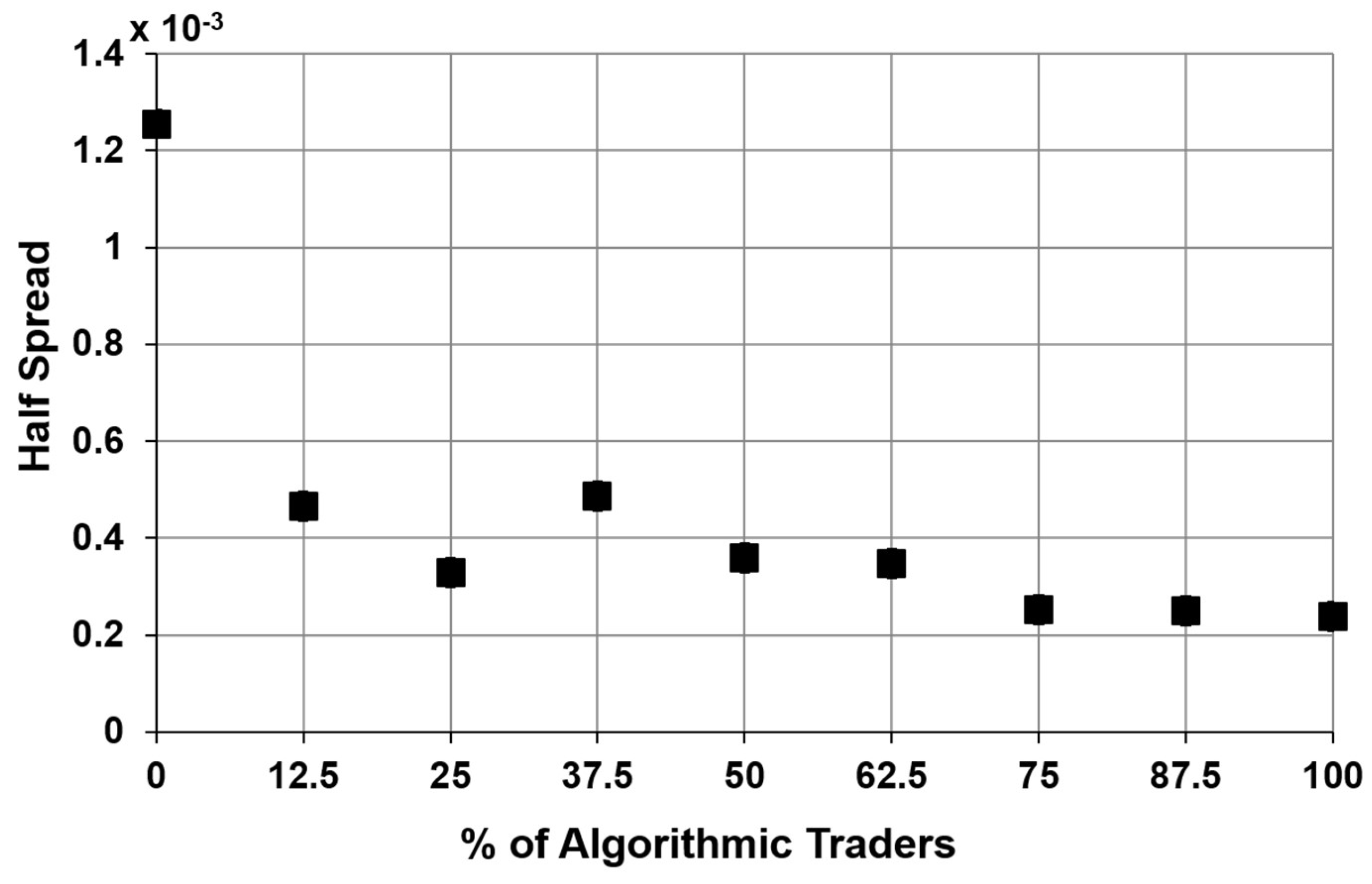
We use effective half-spread as our measure of liquidity (e.g., Hendershott and Riordan 2011). As half-spread decreases, liquidity increases. Half-spread is calculated as:

$$\mathrm{Half}\mathrm{spread}=\left(\mathrm{sign}\right)\frac{(\mathrm{trade}\mathrm{price}-\mathrm{midpoint})}{\mathrm{midpoint}};$$

(6)

where trade price is the price at which trade occurred, midpoint is the price halfway between the transacting bid and ask price, and sign is determined by how the trade was initiated. If a seller initiated the trade then sign = 1, if a buyer initiated the trade then sign = −1. We compute the half spread at 800 evenly distributed points in time over the course of every single 30-day run (see Table 1). At the end of each run, we compute the average half-spread over the recorded 800 values. Each point on the curve in Figure 1 is thus the average of 50 average half spreads (Table 1). We present the results with 95% confidence intervals. For the first point on the graph, our simulation has 1000 human technical traders and 1000 human fundamental traders, with no algorithmic traders. In each successive point of the graph, the proportion of algorithmic traders increases. The number of technical and fundamental traders is equal at all points.

Results indicate that AT has a dramatic liquidity increasing effect early in its adoption. By the time AT reaches 10%, most of the benefit has already been gained. Further increase in the share of AT contributes very little to liquidity. This result indicates an interesting new hypothesis for the empirical literature: as AT presence increases in developing countries, where it is still only a fraction of the total market, empirical studies could estimate if there is a threshold where most of the benefit of AT already accrues to the country. This would provide practical insight into the timeline of AT impact on market quality in developing countries where AT adoption is still at a nascent stage.

4.2. Experiment 2: Statistical Arbitrage/Pairs Trading

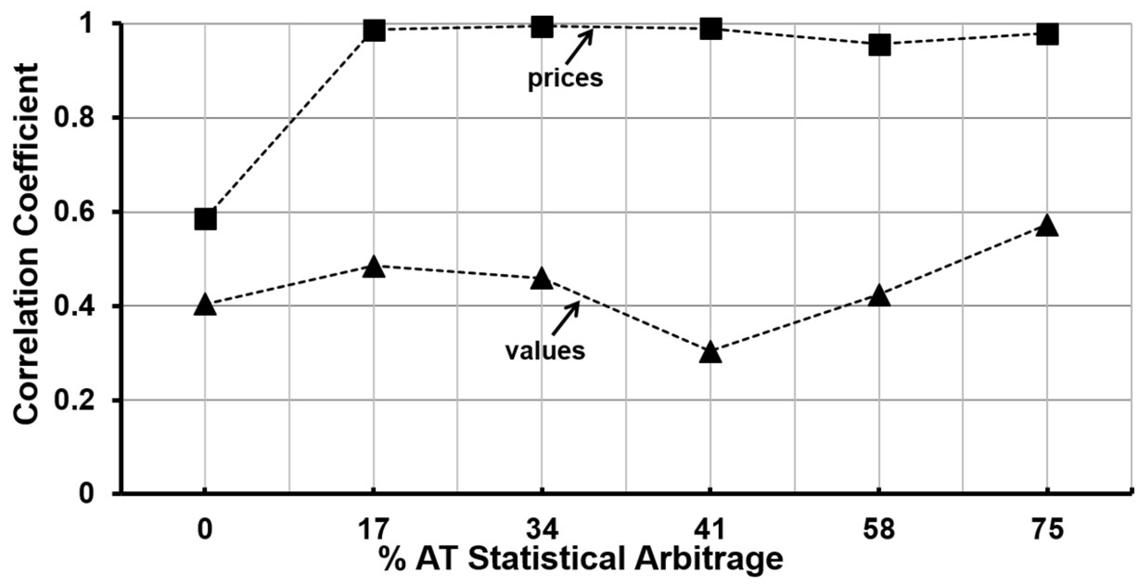
Our goal is to determine the impact of statistical arbitrage/pairs trading. Statistical arbitrage is a strategy to profit by trading based on short-term correlations, while assuming that these correlations will persist. We simulate two fundamentally unrelated (low positive correlation) stocks. We introduce fundamental traders and pairs traders and measure the correlation of the prices and the correlation of the fundamental values of the stocks as the proportion of pairs traders increases.

The results in the form of the correlations between the two paired stocks are shown below in Figure 2. All details of the simulation are given in Table 1. The set-up is similar to Experiment 1 except for the types of traders. Figure 2 shows that the correlation of prices is significantly higher than the correlation in fundamental values of the two stocks. This is in line with empirical findings and anecdotal evidence that indicate AT leading to co-movements in market prices of assets (e.g., Zweig 2010), and price spillovers across assets (e.g., Kelejian and Mukerji 2016), which are above and beyond what fundamentals alone can explain.

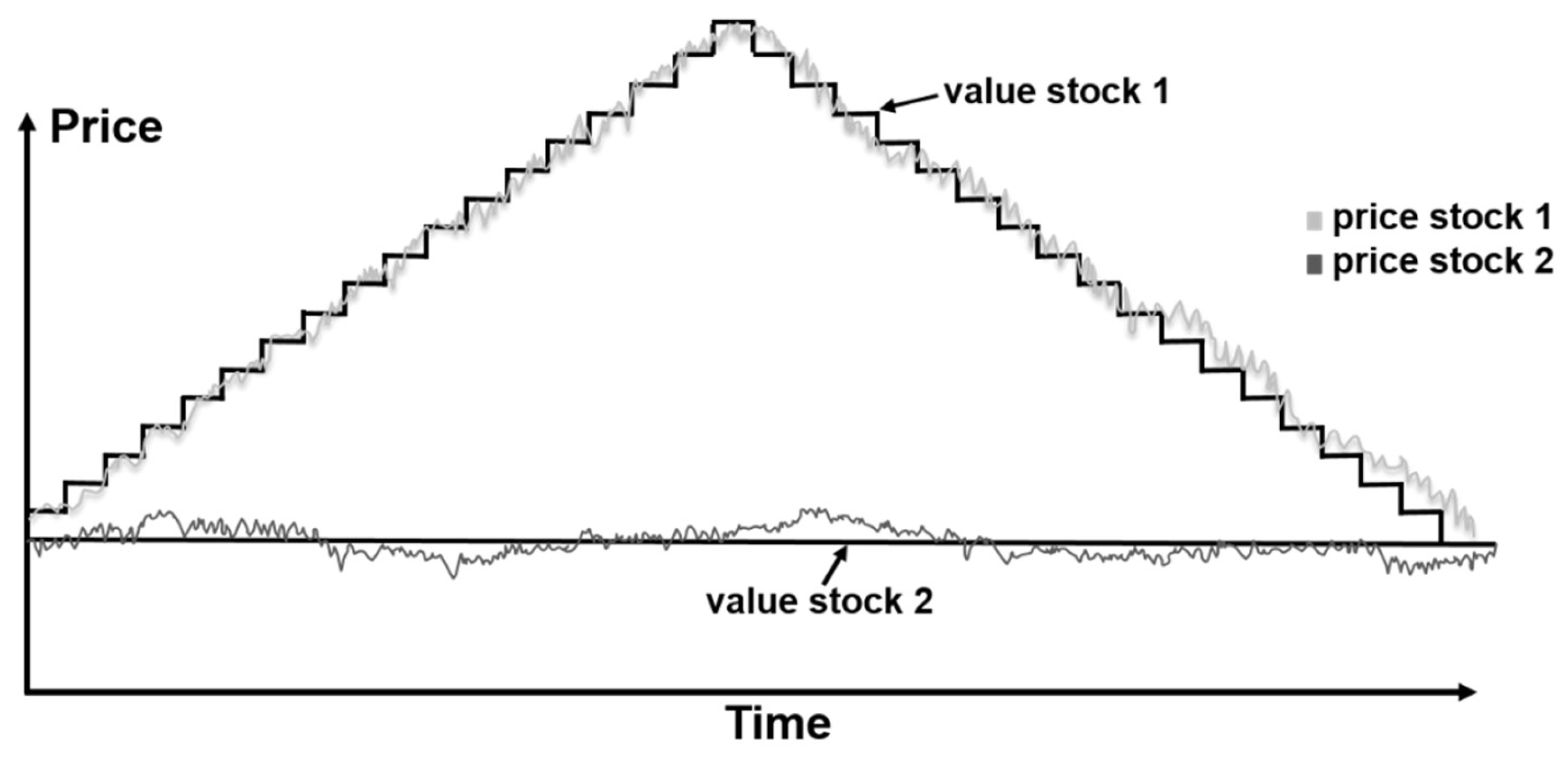
To take a closer look at what unfolds over the course of a typical run, we present Figure 3, which shows what the market looks like when no Pairs traders are present.

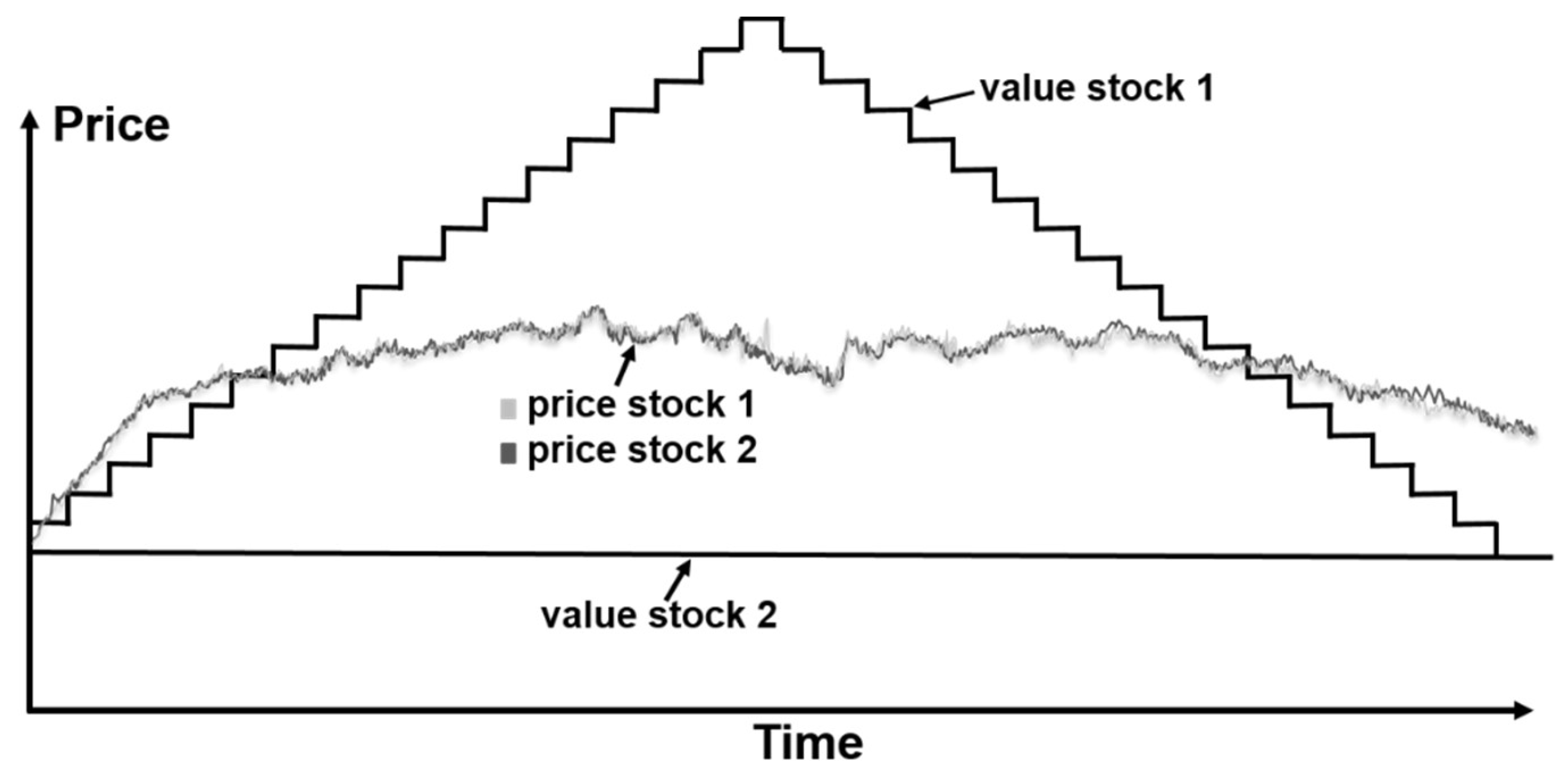
In this run, we control the fundamental values rather than randomly generating them. The first stock’s fundamental value is a step function that increases and then decreases. The second stock’s fundamental value line is the flat line. We see that when there are no Pairs traders, the prices stay near their corresponding fundamental values. In contrast, in Figure 4 we show the same simulation run now with the market comprising 50% algorithmic Pairs traders that trade on the assumption of positive price correlation. The prices in this case are far from their fundamental values and are highly correlated with one another.

This strong impact of AT on prices lends support to findings such as that the initial price impact of an algorithmic trade is larger than that of human orders (Hendershott and Riordan 2011; Hendershott et al. 2011) or that AT contribute significantly to the price discovery process (Brogaard 2010). Our contribution is to show the possibility that the price discovery process might be led astray, due to the strategy combined with the speed of the AT, as we see in Experiment 2.

5. Conclusions

In this paper, we have created a simulated asset market and modeled common AT strategies. We conducted two experiments in this market. Our contribution is the creation of a platform capable of studying the impact of AT trading on market quality directly. This expands our capability of evaluating AT beyond conventional empirical studies. It provides a method of cross-checking empirical findings, gaining deeper insights into them, and also potentially forming new hypotheses for further empirical research.

In Experiment 1, we investigated the impact of AT on market liquidity. We simulated a gradual rise in the participation of AT in a market with fundamental and technical traders of both AT and human types. We found that liquidity rose sharply as AT was introduced with most of the liquidity rise realized at just 10% AT participation. This leads to an interesting hypothesis for future empirical work to see if there is such an early threshold for reaping the liquidity benefits of AT. This could hold important implications for developing countries with nascent AT participation.

In Experiment 2 we investigated the impact of AT on price discovery. We simulated a rise in algorithmic pairs trading that apply statistical arbitrage to make profits based on short-term price correlations. In this experiment, we found high price correlations between the pair traded, even when fundamental values had very little correlation. This supports some findings in the empirical literature that indicate AT leading to price movements away from fundamentals.